Soft Fault Diagnosis of Analog Circuit Based on EEMD and Improved MF-DFA

Abstract

Aiming at the problems of nonlinearity and serious confusion of fault characteristics in analog circuits, this paper proposed a fault diagnosis method for an analog circuit based on ensemble empirical pattern decomposition (EEMD) and improved multifractal detrended fluctuations analysis (MF-DFA). This method consists of three steps: preprocessing, feature extraction, and fault classification identification. First, the EEMD decomposition preprocesses (denoises) the original signal; then, the appropriate IMF components are selected by correlation analysis; then, the IMF components are processed by the improved MF-DFA, and the fault feature values are extracted by calculating the multifractal spectrum parameters, and then the feature values are input to a support vector machine (SVM) for classification, which enables the diagnosis of soft faults in analog circuits. The experimental results show that the proposed EEMD-improved MF-DFA method effectively extracts the features of soft faults in nonlinear analog circuits and obtains a high diagnosis rate.

1. Introduction

At present, although the theory and application of digital signals is closely related to the rapid development of electronic technology, analog signals still occupy an important position. The proportion of analog and digital circuits in hybrid circuits is about 60% and will continue to grow, the data show. Although analog components account for only 20% of hybrid circuits, the cost of testing and diagnosing analog component has reached 80% of the total cost [1]. There are two types of analog circuit fault modes: hard fault and soft fault. Hard faults are catastrophic faults such as an open circuit and short circuit, which are easy to identify, and soft faults are when the parameters of circuit components constantly change and deviate from their nominal values. In the event of a soft fault, the topology of the circuit will not change, but it will affect the performance of the circuit. If the soft fault is not fixed in time, it becomes a hard fault [2]. If so, it can cause a lot of damage to the circuit and even threaten personal safety.

In order to identify soft faults in analog circuits, various diagnostic methods such as the fault dictionary method and the parameter identification method have been proposed by scholars. However, these methods are applicable to only single faults and are much more computationally intensive for diagnosing circuits dealing with multiple faults. With the development of fault diagnosis technology, linear extraction methods such as principal element analysis and factor analysis are proposed successively. These methods are more effective for linear circuits, but most circuits in daily life are nonlinear and the above methods cannot reflect the nonstationary characteristics of signals, which leads to low separability of the extracted fault features, which leads to large classification error in fault pattern recognition. For this reason, scholars have proposed time–frequency domain analysis methods, such as SVM, principal component analysis (PCA), and singular value decomposition (SVD), but each of the above time–frequency domain methods has limitations and shortcomings; for example, the typical fault characteristic parameters of SVM are difficult to choose; PCA is a linear algorithm that cannot accommodate real processes with varying degrees of nonlinearity; the performance of SVD mainly depends on the selection of embedding dimensions; however, the current embedding dimensions are mostly selected empirically and poorly adapted [3,4,5]. In recent years, along with the development of artificial intelligence, more and more artificial intelligence-based methods are applied to the field of circuit fault diagnosis; for example, the literature [6] used artificial neural networks to train and model circuit fault samples, thus improving the circuit fault diagnosis accuracy and shortening the diagnosis time, but artificial neural networks require a large amount of experimental data to form an accurate classification of fault phenomena, while the algorithm converges slowly and is prone to local minima; the literature [7] applied a deep belief network method in deep learning for circuit fault feature extraction. Although it improved the analog circuit fault diagnosis rate, the deep learning model lacks theoretical support in parameter selection and the fault sample library is not rich enough, so there is still much room for improvement in deep learning in nonlinear analog circuit diagnosis. Due to the increasing complexity of electronic systems and the strong coupling of operating states, which leads to the complexity and diversity of their fault patterns, and sometimes even chaos, the traditional theories and methods to portray this complexity increasingly feel the limitations of the theory itself. The fractal theory developed in recent years has provided a good idea for solving this problem. Sheng et al. [8] combined local characteristic-scale decomposition with fractal theory to effectively extract fault features of analog circuits and achieve fault diagnosis of analog circuits. Yao et al. [9] used fractal theory and probabilistic neural networks to implement fault diagnosis of miniature circuit breakers. Mao et al. [10] proposed the method of combining support vector machines with fractal theory and obtained good results. However, the fractal in the above methods is a single fractal. A single fractal can only describe the fractal characteristics of the signal from one perspective, which is not comprehensive enough to describe the fractal characteristics of the signal and cannot portray the local fractal characteristics of the signal. In fault diagnosis, it is difficult to achieve accurate classification and identification once there are intervals where the dimensions of different state signals overlap. The improved MF-DFA method proposed in this paper analyzes from multiple scales to comprehensively respond to the distribution of nonuniformity and probability measures of the structure of fractal objects and provides a more refined description of local fractal features. At the same time, because the actual measured signals are often accompanied by abnormal events, such as noise effects, intermittent signals, etc., leading to the occurrence of the phenomenon of modal aliasing, which has a great impact on the subsequent fault diagnosis rate, this paper thus proposes the EEMD method to preprocess the signal, which can effectively avoid the phenomenon of modal aliasing.

In summary, an analog circuit fault signal state identification method based on EEMD and improved MF-DFA was proposed in this paper. Firstly, EEMD of the circuit fault signal was carried out to obtain several IMF components with no mode overlap; then, the IMF components with circuit fault signal characteristics were selected to reconstruct the fault signal according to the circuit fault characteristics. Later, the fault signal was analyzed by the improved MF-DFA, the Hurst exponent and multifractal spectrum of the fault signal were obtained, and the multifractal spectrum width, extreme value, dimension difference and generalized Hurst exponent fluctuation mean of fault signal were calculated to the characteristic parameters of circuit fault state. Finally, the feature parameters extracted from the improved MF-DFA were classified by SVM to realize the diagnosis of the analog circuits’ soft fault.

The rest of this paper is organized as follows: Section 2 presents the signal preprocessing method (EEMD). The signal feature extraction method (improved MF-DFA) is proposed in Section 3. Section 4 contains the experimental simulations and results. Section 5 contains the conclusion.

2. EEMD

EMD is an effective method for processing circuit fault signals. EMD has the adaptive property of delocalizing time-varying features, which can decompose the signal into the sum of several IMF and reduce the coupling of feature information between signals. By decomposing the signal by EMD method, we can grasp the characteristic information of the original data accurately and efficiently, which is helpful for the mining of information characteristics [11]. However, EMD leads to modal confusion in circuit signal decomposition. To this end, Wu et al. [12] proposed a new method, namely EEMD, in which the unstable signal is decomposed by EEMD to obtain a stationary IMF, effectively avoiding modal confusion.

The essence of EEMD is to superimpose circuit fault signal with Gaussian white noise, and then to EMD decompose it several times, using Gaussian white noise with statistical properties of uniform frequency distribution to make the circuit fault signal have continuity at different scales, thus reducing the degree of mode confounding of each IMF component [13]. In EEMD decomposition, the decomposed circuit fault signal components are averaged through several iterations, and the more the averaging process, the less noise interferes with the decomposition results and the more useful signals can be highlighted. Set the average number of times the original fault signal is processed to N, initially 1, 2, …, N. The decomposition of EEMD is as follows:

(1) Gaussian white noise ${\rho }_i(t)$ is added to the original circuit fault signal $x(t)$ to obtain the signal $x_i(t)$:

$$x_i(t)=x(t)+{\rho }_i(t)$$

(1)

(2) The fault signal components IMF at different scales are obtained by EMD decomposition:

$$x_i(t)={\displaystyle \sum _{i=1}^{n}IM{F}_{i,n}(t)+r_{i,n}(t)}$$

(2)

where n is the number of IMFs after EMD decomposition; $r_{i,n}(t)$ is the residual component.

(3) $x(t)$ adds different Gaussian white noise and repeats steps (1) and (2), N is the number of clusters, so when the number of noise added is equal to the number of clusters, then the iteration of the algorithm is stopped. The results of EEMD decomposition are as follows:

$$x(t)={\displaystyle \sum _{k=1}^{n}IM{F}_{k,n}(t)+r_{k,n}(t)}$$

(3)

(4) Averaging of the IMF components after EEMD decomposition to eliminate noise interference with the signal:

$$IM{F}_n(t)=\frac{1}{N}{\displaystyle \sum _{K=1}^{N}IM{F}_{kn}(t)}$$

(4)

The error between the reconstructed signal obtained using the sum of $IM{F}_n(t)$ and the original signal satisfies the following equation:

$${\omega }_n=\frac{\omega }{\sqrt{N}}$$

(5)

N is the average number of times EEMD; $\omega$ is the standard deviation of the added white noise; and as can be seen from the equation above, ${\omega }_n$ decreases with the increase of the total N. It is known from several tests that the decomposition effect is best when $\omega$ is 0.2 and N is 100.

The flow chart of EEMD signal decomposition is shown in Figure 1.

As can be seen from Figure 1, after the input excitation signal, we first add Gaussian white noise to the original signal several times, then we separately perform EMD decomposition on the signal after adding Gaussian white noise, and finally we statistically average the IMF components obtained after EMD decomposition to obtain the final IMF components. In order to eliminate the effect of noise confusion, we performed the above process for each circuit signal.

3. Improved MF-DFA

The MF-DFA method is a nonstationary time series multiple fractal characterization method based on the detrended fluctuation analysis (DFA) method proposed by Kantelhard J. w. et al. This method firstly eliminates the influence of the nonstationary trend of fault signal sequence by de-volatility process and then describes the fractal structure of time series in different dimensions by calculating the volatility functions of different order. Compared to the DFA method, the MF-DFA method avoids human-induced effects and can more accurately characterize the multiple fractal features hidden in non-stationary time series [14]. For a circuit fault signal sequence $x(n)$ of length N, the steps for MF-DFA are as follows:

(1) Calculate the cumulative deviation $y(n)$ of the fault signal sequence $x(n)$:

$$y(n)={\displaystyle \sum _{i=1}^n\left(x(i)-\overline{x}\right)},n=1,2,\dots ,N$$

(6)

where $x(n)$ is the original fault signal sequence and $\overline{x}$ is the average value of the signal, $\overline{x}=\frac{1}{N}{\displaystyle \sum _{i=1}^{N}x(i)}$.

(2) The traditional MF-DFA method uses the equal sequence partitioning method, which divides the cumulative deviation sequence $y(n)$ into m equal-length sequences without overlapping each other on average, where the data length of each subsequence is s. When N cannot divide s integerly, to avoid data remainder, the sequence is partitioned again from the end of the sequence, and finally 2m equal-length subsequences are obtained. This leads to data discontinuity at the segmentation point of the fault signal subsequence, generating new pseudo-volatility errors, and there is a risk of losing the data at the end of the circuit fault sequence or disrupting the order of the original fault signal sequence in the process of constructing the subsequence, resulting in distortion of the estimated generalized Hurst index. In order to overcome the shortcoming of the traditional MF-DFA method, the sliding window technique is introduced to improve the MF-DFA sequence segmentation method. The principle of the sliding window segmentation method shown in Figure 2.

In order to minimize the data discontinuity at the segmentation point of the fault signal subsequence and the risk of losing the data at the end of the circuit fault sequence or disrupting the order of the original fault signal sequence in the process of constructing the subsequence, this paper uses an overlapping window for segmenting the data sequence.

The sliding window overlap segmentation method results in an increase in the segmented subsequences from m or 2m to N-s + 1 (to avoid remaining data at the end, step r = 1).

(3) The local trend function of each subsequence is fitted with least-squares:

$$y_v(n)=a_0+a_{1}n+a_2{n}^2+\dots +a_k{n}^k,n=1,2,\dots ,2m;k=1,2,\dots$$

(7)

where $a_k$ is the coefficient of the polynomial fit and k is the order of the polynomial fit.

The polynomial fitting process is prone to underfitting and overfitting problems. Underfitting occurs generally because the complexity of the model used is too low and the amount of features used is too small. In this paper, because the circuit model is fixed, the number of features in the sample is increased by polynomial regression in this paper so as to solve the error problem caused by overfitting. Overfitting occurs due to a single sample of training data set, insufficient samples, and too much noise interference in the training process, so this paper selects data samples with positive and negative deviations to ensure the diversity of samples, while using the EEMD method to denoise the samples, which greatly avoids the test error caused by overfitting.

(4) Calculate the mean square error function when v = 1, 2, 3, …, m, with

$$F^2(s,v)=\frac{1}{s}{\displaystyle \sum _{n=1}^s{\left\{y\left[(v-1)s+n\right]-y_v(n)\right\}}^2}$$

(8)

When v = m + 1, m + 2, …, 2m,

$$F^2(s,v)=\frac{1}{s}{\displaystyle \sum _{n=1}^s{\left\{y\left[N-(v-1)s+n\right]-y_v(n)\right\}}^2}$$

(9)

(5) Traditional MF-DFA calculates the q-rung fluctuation function:

$$F(q,s)={\left\{\frac{1}{2m}{\displaystyle \sum _{v=1}^{2m}{\left[F^2(s,v)\right]}^{q/2}}\right\}}^{1/q},q\ne 0$$

(10)

$$F(q,s)=\exp \left\{\frac{1}{4m}{\displaystyle \sum _{v=1}^{4m}\ln \left[F^2(s,v)\right]}\right\},q=0$$

(11)

Improved MF-DFA to calculate the q-rung fluctuation function:

$$F(q,s)={\left\{\frac{1}{N-s+1}{\displaystyle \sum _{v=1}^{N-s+1}{\left[F^2(s,v)\right]}^{q/2}}\right\}}^{1/q},q\ne 0$$

(12)

$$F(q,s)=\exp \left\{\frac{1}{2(N-s+1)}{\displaystyle \sum _{v=1}^{N-s+1}\ln \left[F^2(s,v)\right]}\right\},q=0$$

(13)

To ensure high stability of the fluctuation function $F(q,s)$, the fixed window length is 2k + 2< s < int (N) (in which k is the polynomial fitting order).

(6) the order q takes a certain value in turn, the scale s takes different values, and repeat steps (2)–(5) to calculate the double logarithmic value of F(q,s) for q.

(7) The fluctuation function is a function on the data length q and the subsequence data length s, which is related to s as shown below:

$$F(q,s)\propto s^{h(q)}$$

(14)

(8) The relationship between generalized Hurst index $h(q)$ and scalar index $\tau (q)$ obtained by MF-DFA method is as follows:

$$\tau (q)=qh(q)-1$$

(15)

Both sides of Equation (15) are simultaneously derived for q:

$$\frac{d\tau (q)}{dq}=h(q)+q{h}^{\prime }(q)$$

(16)

The relationship between the multiple fractal spectrum $f(a)$, the singularity index $a$ and the scalar index $\tau (q)$ is obtained by the Lejeune transform:

$$\{\begin{array}{l}a=\frac{d\tau (q)}{dq}\\ f(a)=aq-\tau (q)\end{array}$$

(17)

Substituting Equation (15) into Equation (16) yields the following relationship:

$$\{\begin{array}{l}a=h(q)+q{h}^{\prime }(q)\\ f(a)=q[a-h(q)]+1\end{array}$$

(18)

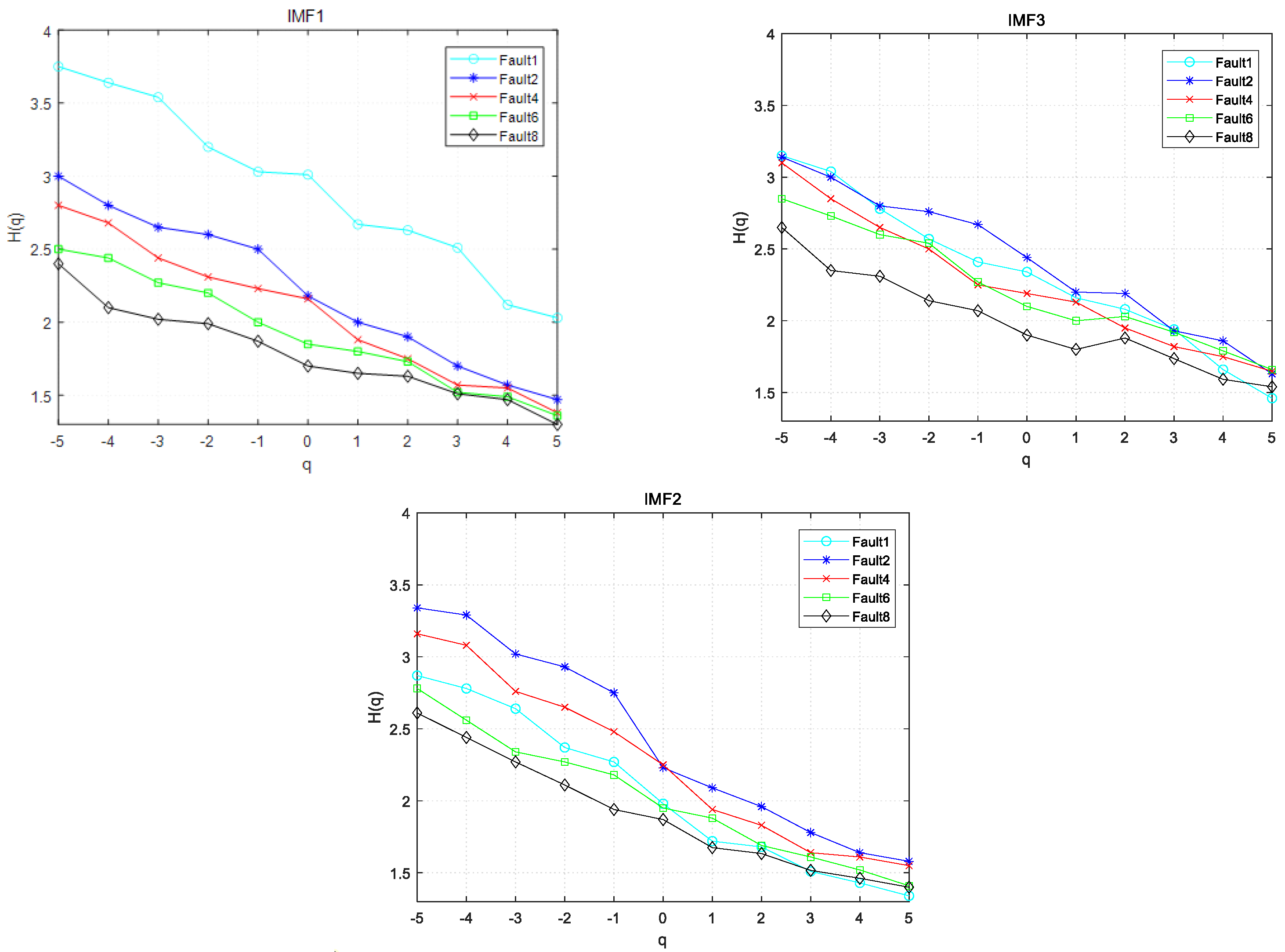
The generalized Hurst index reflects the relationship between the different scales of circuit signal and is a characteristic measure of the multifractal characteristics of circuit signal. In a coordinate system with $q$ as horizontal and $h(q)$ as vertical, if $q$ and $h(q)$ are a nearly smooth straight line, the circuit signal has no multifractal characteristics; if $q$ and $h(q)$ are a non-linear decreasing function, the circuit signal has multifractal characteristics, and the more $h(q)$ fluctuates, the stronger the multifractal characteristics of the circuit signal. Therefore, the generalized Hurst exponent fluctuation mean is taken as one of the fault’s characteristics.

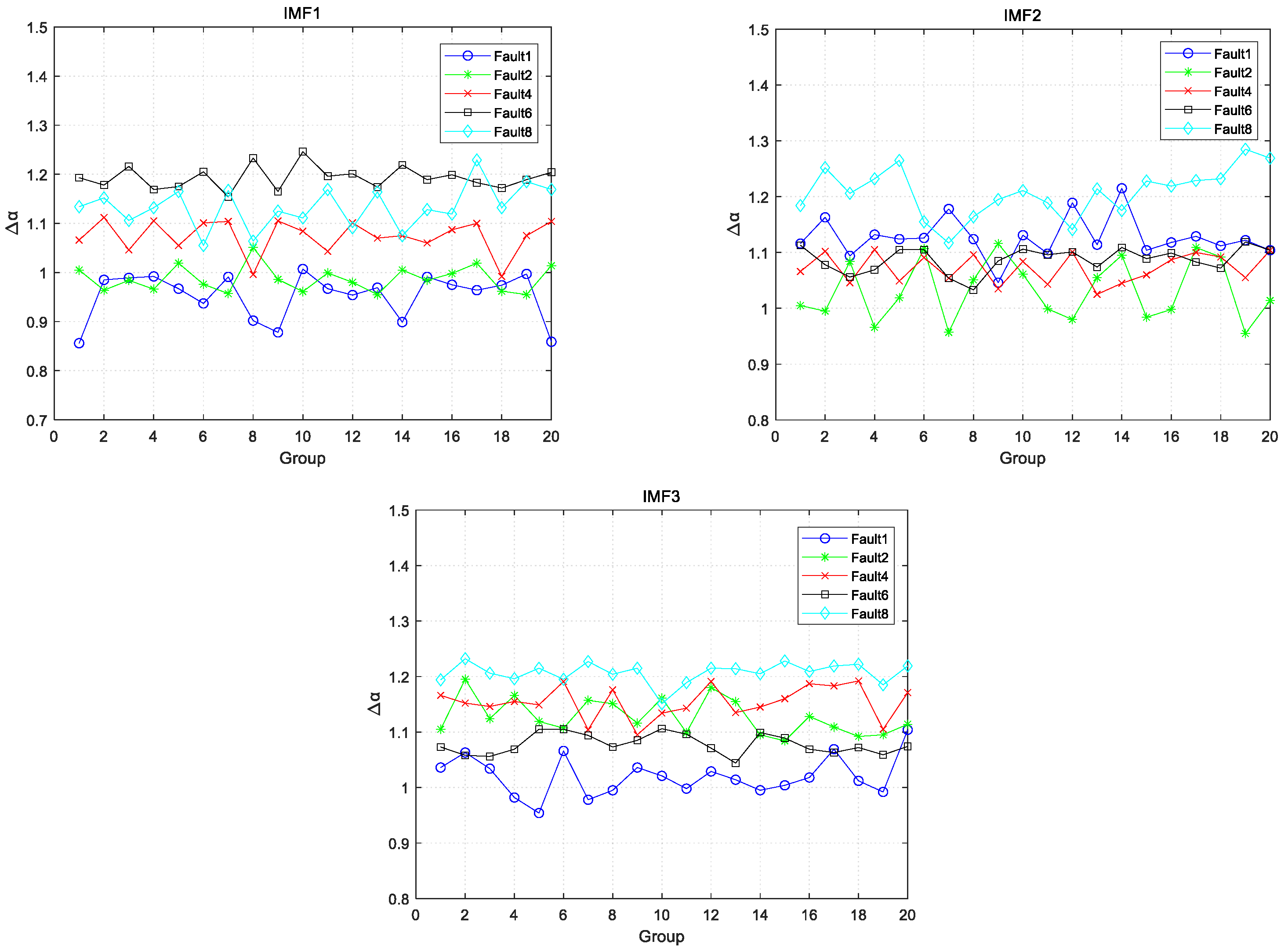
The width of the multifractal spectrum $\Delta a$ is the difference between the strongest and weakest singularities of the signal, reflecting the strength of the multifractal characteristics of the circuit signal; the stronger the multifractal characteristics, the larger the value of $\Delta a$; for the singularity index $a_0(f_{\max }=f(a_0))$ corresponding to the extreme value point, which reflects the randomness of the circuit signal, the greater the randomness, the greater the $a_0$; the difference between the fractal dimension of the maximum and minimum probability subsets $\Delta f$ = $f(a_{\max })-f(a_{\min })$, reflecting the change in the maximum and minimum peak frequencies of circuit signal, which is less than 0, indicating that the number of maximum probability subsets is greater than the number of minimum probability subsets, and vice versa. Through the above analysis, it can be seen that the multiple fractal spectrum parameters can reflect the intrinsic characteristics of a fault signal in different states quantitatively; therefore, four characteristic parameters are proposed as circuit fault state identification parameters.

As can be seen from Figure 3, after the original signal is processed by EEMD, a number of IMF components are obtained. The IMF components without mode overlap are selected by correlation calculation. Then, we calculate the cumulative deviation of these IMF components, and then cut the cumulative deviation sequence by sliding window to obtain N-S + 1 subseries, and then calculate the mean square error function and q-rung fluctuation function by polynomial fitting of these subseries, and finally obtain the multifractal spectrum of the fault signal by the q-rung fluctuation function, so as to calculate the multifractal spectrum parameters as eigenvalues into the support vector machine.

4. Simulation Experiment

4.1. Experimental Process

Figure 4 provides the flow chart of analog circuit fault diagnosis based on the EEMD-improved MFDFA.

The steps of the EEMD-improved MFDFA-based analog circuit fault diagnosis are as follows:

(1) Apply an excitation signal to the circuit to be tested, select the fault component by sensitivity analysis, and collect the output response under different fault modes for signal preprocessing.

(2) EEMD decomposition is performed on the acquired signal data to obtain each IMF component.

(3) Each IMF component is processed by improved MF-DFA to obtain the width, extreme value, dimensional difference and generalized Hurst index fluctuation mean of the multiple fractal spectrum of the fault signal, which constitutes the fault feature vector.

(4) The SVM is extended with a “one-to-many” approach for multi-classification.

(5) The training samples are input to the classifier for training, and the trained classifier is used to classify and diagnose the fault data.

4.2. Experimental Environment

In order to verify the validity of the experimental method, a circuit model was established in NI Multisim 14.0 using the bandpass filter circuit in Figure 5 as a diagnostic example, and data were processed with MATLAB R2021b. The parameters of the circuit components are shown in Figure 5. Resistance tolerance was set at 5% and capacitor tolerance at 10%, and the parameters of each element were considered to be in normal condition in this range, with more than 30% considered to be fault state.

The excitation signal for this experiment was f (t) = sin (800πt) + sin (sin (1000πt)) + sin (sin (2800πt)) + noise. A total of ten kinds of parameter-type fault combinations were configured. The failure of amplifier is affected by many factors, so it is not discussed here. The fault mode settings are shown in

Table 1. Circuit failure modes of bandpass filters.

Fault Code	Fault State	Nominal Value	Fault Value
1	Normal	-	-
2	R2↑30%	1 kΩ	1.3 kΩ
3	R2↓30%	1 kΩ	0.7 kΩ
4	R3↑30%	3 kΩ	3.9 kΩ
5	R3↓30%	3 kΩ	2.1 kΩ
6	C1↑30%	5 nF	6.5 nF
7	C1↓30%	5 nF	3.5 nF
8	C2↑30%	5 nF	6.5 nF
9	C2↓30%	5 nF	3.5 nF

.

4.3. Experimental Result

Multisim simulation software was used to analyze the circuit instantaneously and sample the output response to obtain the original fault information. Fifty Monte Carlo analyses were performed for each type of the fault in Table 1, and the samples under each failure mode were randomly divided into two parts, with 30 sets of data participating in training and the other 20 sets of data for testing.

All sample data were decomposed by EEMD, and the results are provided in Figure 6 and Figure 7 for the normal mode and the fault 7 mode. By comparing Figure 6 and Figure 7, it can be seen that the fault information is mainly concentrated in the first three IMF components, so the first three components are selected for feature parameter extraction.

The following is an example of fault 1, fault 2, fault 4, fault 6, and fault 8, and the number of samples for each state was selected as 50 for a total of 150 groups of samples. The improved MF−DFA was applied to the IMF components, and the order q range was taken as [−5, 5], and a total of 11 q values were taken. The Hurst index curve and the multifractal spectrum were obtained, as shown in Figure 8 and Figure 9. As can be seen from Figure 8, the generalized Hurst exponents of five signals is a curve of about q, indicating that the circuit signals of these five circuit states have multiple fractals characteristics. It can be seen from Figure 9 that the singular spectra of the five signals have different shapes, positions, and spectral widths. Based on the characteristic of singularity spectrum, the multiple fractal features of signal can be extracted further, and the fault diagnosis can be carried out effectively.

To further highlight the advantages of the improved MF−DFA, the traditional MF-DFA was used in this paper to process the sample signals in five states under three IMF components, with scalar values and order q being the same as the improved MF−DFA settings, resulting in the Hurst curve, and the results are shown in Figure 10.

From Figure 8 and Figure 10, it can be seen that the generalized Hurst curve index decreases with increasing value of q for both MF−DFA and improved MF−DFA methods, indicating the existence of irregular multiple fractal characteristics of the circuit signal. At q < 0, the h(q) value of the improved MF−DFA method is smaller than that of the conventional method, while at q > 0, the h(q) value of the improved MF−DFA method is greater than that of the conventional method, suggesting that the improved MF−DFA method can effectively reduce the pseudorandom fluctuation error caused by the discontinuity of time series segmentation point, while avoiding tail data loss and sequence reconstruction errors of the conventional method.

The average values of the multifractal spectral parameters for each of the five states of the circuit were calculated using the improved MF−DFA method, as shown in

Table 2. Multifractal spectral parameter averaging based on improved MF−DFA.

	Fault Code	$\mathbf{\Delta }\mathit{a}$	${\mathit{a}}_0$	$\mathbf{\Delta }\mathit{f}$	$\mathbf{\Delta }\overline{\mathit{h}}(\mathit{q})$
IMF1	1	0.956	2.098	0.809	2.947
	2	0.996	0.815	0.386	2.315
	4	1.103	0.752	0.474	2.085
	6	1.201	0.697	0.641	1.929
	8	1.134	0.636	0.714	1.713
IMF2	1	1.083	0.832	0.324	2.179
	2	1.036	0.932	0.432	2.412
	4	1.072	0.894	0.531	2.297
	6	1.087	0.771	0.645	2.031
	8	1.155	0.694	0.725	1.765
IMF3	1	1.021	0.913	0.321	2.419
	2	1.132	0.986	0.431	2.534
	4	1.154	0.837	0.590	2.274
	6	1.076	0.759	0.521	2.116
	8	1.207	0.709	0.708	1.878

. Meanwhile, the distributions of $\Delta a$, $a_0$, $\Delta f$, and $\Delta \overline{h}(q)$ for the five states are shown in Figure 11, Figure 12, Figure 13 and Figure 14. From the figure, it can be seen that $\Delta f$ and $\Delta \overline{h}(q)$ have subtle crossover in different states, while $\Delta a$ and $a_0$ were mixed severely, so $\Delta f$ and $\Delta \overline{h}(q)$ were selected to form the eigenvectors in this paper.

To further verify the effect of the proposed feature extraction method, SVM was used to model and classify the extracted features. Each state had 30 samples for SVM training and the remaining 20 samples for testing. We also compared with the wavelet packet energy spectrum and ICA (WP−ICA)-based analog circuit fault feature extraction method from the literature [15] and the EEMD multiscale entropy and LSSVM (EEMD−LSSVM) in the analog circuit fault diagnosis method from the literature [16]; the diagnosis results of the three methods were obtained, as shown in

Table 3. Fault diagnosis results of three methods.

	WP−ICA	EEMD−LSSVM	EEMD−Improved-MFDFA
Average detection rate/%	95.7	96.67	97.87

.

In this paper, $\Delta f$ and $\Delta \overline{h}(q)$ were input to the support vector machine as feature vectors for classification. The classification results are shown in Table 3. In the same circuit environment, the recognition rate of the proposed method in this paper can reach 97.87%, while the recognition rates of the other two methods are 95.7% and 96.67%. This shows that the method proposed in this paper has more advantages in circuit soft fault identification.

In order to better verify the effectiveness of the method in this paper, the method in this paper is used in the fault feature extraction of three different circuits, namely, Sallen–Key lowpass filter, state-variable filter, and active dual second-order bandpass filter, and compared with the CBAM−CNN analog circuit fault diagnosis method from the literature [17], the FFT−CNNN−GRU analog circuit fault diagnosis method from the literature [18], and the MLLE−CHMM analog circuit fault diagnosis method from the literature [19]. The diagnosis results are shown in the following table.

From

Table 4. Diagnostic results of the corresponding methods under the three circuit models.

Circuit Models	Method	Diagnosis Rate (%)
Sallen–Key lowpass filter	EEMD-Improved MF-DFA	96.31
	CBAM-CNN	95.48
State-variable filters	EEMD-Improved MF-DFA	97.785
	FFT-CNN-GRU	97.778
Active dual second-order bandpass filter	EEMD-Improved MF-DFA	96.32
	MLLE-CHMM	95.04

, it can be seen that the method in this paper is still very effective in circuit fault feature extraction even under different circuit models, while the diagnosis rate shows that the method in this paper is more advantageous than other methods with higher recognition rate.

5. Conclusions

Aiming at the difficulty of analog circuit fault diagnosis feature extraction caused by the nonlinearity and non-smoothness of analog circuit fault signal, an improved MFDFA fault diagnosis method based on EEMD was proposed. In order to avoid the problem of signal confusion, EEMD decomposition was used to preprocess each fault signal to obtain three IMF components without mode confusion, and then the improved MF-DFA processing of the obtained IMF components to obtain the multifractal spectrum. Because the multifractal spectra corresponding to different fault features have different shapes, distributions, and pole positions, they can be used to characterize different types of circuit faults. Subsequently, this paper used the $\Delta f$ and $\Delta \overline{h}(q)$ obtained from the multiple fractal spectrum to form the feature vectors, and finally the support vector machine analysis method was used to classify the fault features. The results proved that the proposed EEMD-improved MFDFA-based fault feature extraction method showed good performance.

References

1. Khemani, V.; Azarian, M.H.; Pecht, M.G. Learnable Wavelet Scattering Networks: Applications to Fault Diagnosis of Analog Circuits and Rotating Machinery. Electronics 2022, 11, 451. [Google Scholar] [CrossRef]
2. El-Gamal, M.A.; Hassan, A.K.S.O.; Ibrahim, A.A.I. Analog Fault Diagnosis Using Conic Optimization and Ellipsoidal Classifiers. J. Electron. Test. 2014, 30, 443–455. [Google Scholar] [CrossRef]
3. Yang, Z.; Tian, Y.; Deng, N. Leave-One-Out Bounds for Support Vector Ordinal Regression Machine. Neural Comput. Appl. 2008, 18, 731–748. [Google Scholar] [CrossRef]
4. Wang, Y.P.; Mei, F.; Zheng, J.Y.; Mei, J. Research on Fault Diagnosis of High-Voltage Circuit Breaker in Electrical Power System Based on KPCA. Adv. Mater. Res. 2013, 676, 269–272. [Google Scholar] [CrossRef]
5. Cui, L.L.; Liu, Y.H.; Wang, X. Feature Extraction of Weak Fault for Rolling Bearing Based on Improved Singular Value Decomposition. J. Mech. Eng. 2022, 58, 156–169. [Google Scholar]
6. Narula, A.K.; Singh, A.P. Fault Diagnosis of Mixed-Signal Analog Circuit using Artificial Neural Networks. Int. J. Intell. Syst. Appl. 2015, 7, 11–17. [Google Scholar] [CrossRef] [Green Version]
7. Wang, X.L.; Li, C.; Zhang, C.L. Analog Circuit Fault Diagnosis Method Based on Deep Learning. Chin. J. Electron Devices 2019, 42, 674–678. [Google Scholar]
8. Sheng, P.; Xu, A.Q.; Xu, X.W.; Li, H. Fault Diagnosis Method of Analog Circuit Based on LCD and Fractal Dimension. J. Nav. Aeronaut. Astronaut. Univ. 2020, 35, 101–105+118. [Google Scholar]
9. Yao, Y.; Wang, N. Fault Diagnosis Model of Adaptive Miniature Circuit Breaker Based on Fractal Theory and Probabilistic Neural Network. Mech. Syst. Signal Process. 2020, 142, 106772. [Google Scholar] [CrossRef]
10. Mao, J.K.; Mao, X.B. Application of SVM Classifier and Fractal Feature in Circuit Fault Diagnosis. Adv. Mater. Res. 2012, 490–495, 942–945. [Google Scholar] [CrossRef]
11. Chen, K.; Zhou, X.C.; Fang, J.Q.; Zheng, P.; Wang, J. Fault Feature Extraction and Diagnosis of Gearbox Based on EEMD and Deep Briefs Network. Int. J. Rotating Mach. 2017, 2017, 9602650. [Google Scholar] [CrossRef] [Green Version]
12. Wu, Z.; Huang, N.E. Ensmble Empirical Mode De-composition: A Noise—Assisted Data Analysis Method. Adv. Adapt. Data Anal. 2009, 1, 1–41. [Google Scholar] [CrossRef]
13. Singh, S.K.; Kumar, S.; Dwivedi, J.P. Compound Fault Prediction of Rolling Bearing Using Multimedia Data. Multimed. Tools Appl. 2017, 76, 18771–18788. [Google Scholar] [CrossRef]
14. Liu, H.; Jing, J.; Ma, J. Fault Diagnosis of Electromechanical Actuator Based on VMD Multifractal Detrended Fluctuation Analysis and PNN. Complexity 2018, 2018, 9154682. [Google Scholar] [CrossRef]
15. Shan, S.S.; Ma, Q.F.; Xie, W.X. Fault Feature Extraction of Analog Circuit Based on Wavelet Packet Energy Spectrum and ICA. Electron. Meas. Technol. 2021, 44, 19–23. [Google Scholar]
16. Zhuang, C.C.; Yi, H.; Zhang, J. Application of EEMD Multi-Scale Entropy and LSSVM in Analog Circuit Fault Diagnosis. Microelectron. Comput. 2019, 36, 78–82. [Google Scholar]
17. Du, X.J.; Gong, B.; Yu, P.; Shi, Y.K. CBAM-CNN based analog circuit fault diagnosis. Control Decis. 2022, 37, 2609–2618. [Google Scholar]
18. Liu, Y.P.; Xu, W.Z.; Yang, Q. Diagnosis Method of Analog Circuit Fault Based on FFT-CNN-GRU. J. Shenyang Ligong Univ. 2021, 40, 27–30+65. [Google Scholar]
19. Chen, S.; Zhang, M.L.; Zhang, S.; Qiu, X.X.; Xu, C.W. MLLE-CHMM Based Fault Diagnosis Method for Analog Circuits. Mod. Ind. Econ. Inf. 2022, 12, 302–304+311. [Google Scholar]
Figure 1. EEMD signal decomposition flow chart.
Electronics 12 00114 g001
Figure 2. Sliding window principle.
Electronics 12 00114 g002
Figure 3. Flow chart of improved MF-DFA algorithm.
Electronics 12 00114 g003
Figure 4. Basic flow chart for soft fault diagnosis of analog circuits.
Electronics 12 00114 g004
Figure 5. Bandpass filter circuit.
Electronics 12 00114 g005
Figure 6. EEMD decomposition of the signal in normal condition.
Electronics 12 00114 g006
Figure 7. EEMD decomposition of the signal corresponding to fault 7.
Electronics 12 00114 g007
Figure 8. Hurst curves under five signals based on improved MF−DFA.
Electronics 12 00114 g008
Figure 9. Multiple fractal spectral curves under five signals based on improved MF−DFA.
Electronics 12 00114 g009
Figure 10. Five signal Hurst curves based on conventional MF−DFA.
Electronics 12 00114 g010
Figure 11. Distribution of Δa in five fault modes.
Electronics 12 00114 g011
Figure 12. Distribution of a0 in five fault modes.
Electronics 12 00114 g012
Figure 13. Distribution of Δf in five fault modes.
Electronics 12 00114 g013
Figure 14. Distribution of Δ h ¯ ( q ) in five fault modes.
Electronics 12 00114 g014