
Unsupervised and Self-Supervised Tensor Train for Change Detection in Multitemporal Hyperspectral Images


Abstract
:1. Introduction
- (1).
- Inspired by the knowledge from quantum information theory, this work theoretically proves that TT decomposition exhibits greater ability than the traditional TD in capturing global correlations between changed and unchanged tensor entries. Thus, TT is used to extract spectral–spatial low-rank features for multitemporal HSI CD, which decomposes a high-order tensor into a set of low-order tensors by approximating the optimal TT rank.
- (2).
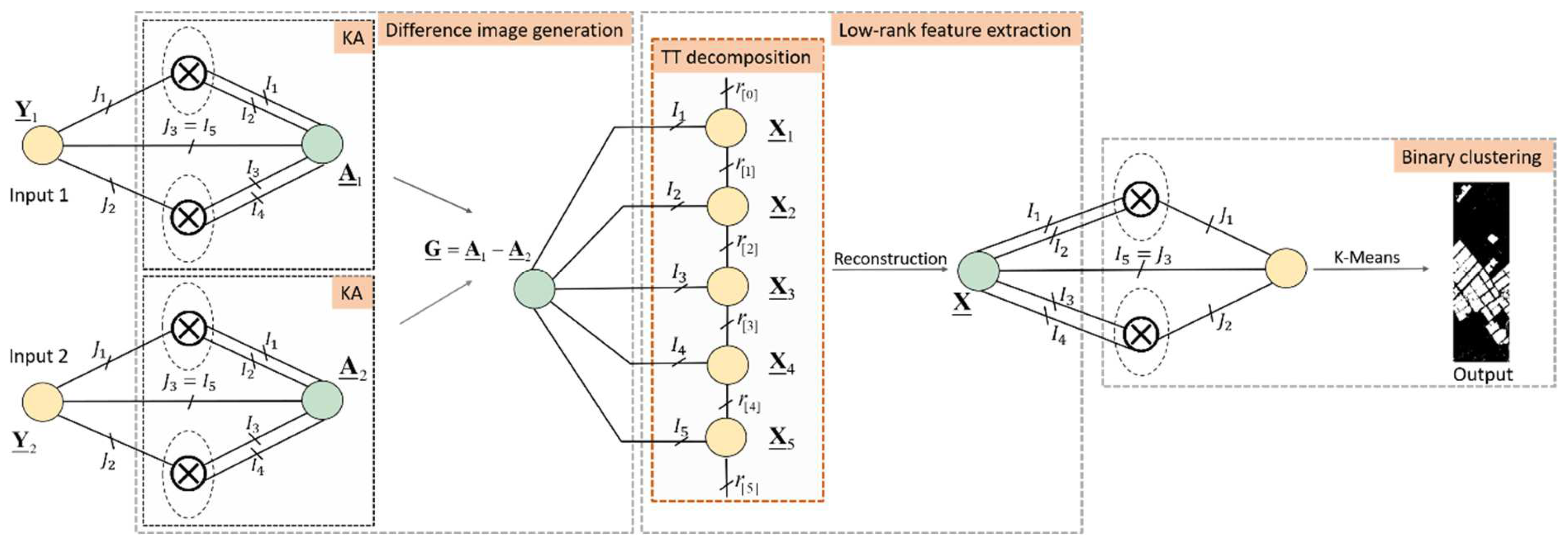
- KA is used to obtain higher-order tensor representations of changed features. This technique leverages the representation of changed features and provides discriminative information for CD while retaining the total number of entries.
- (3).
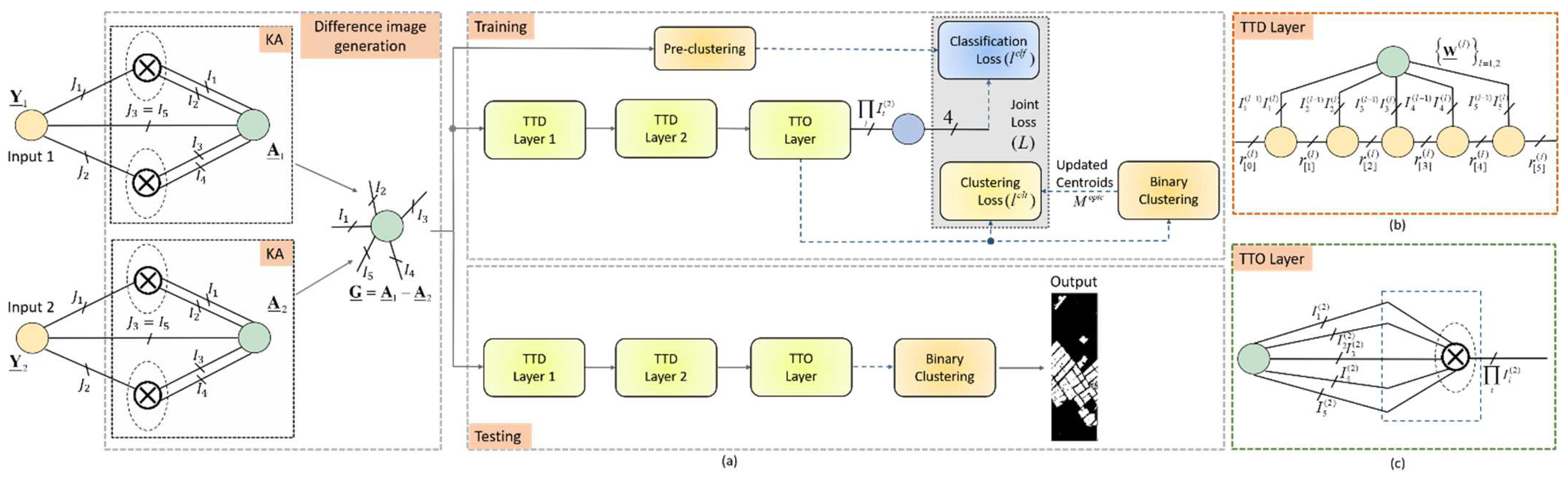
- Two novel TT models that do not require manual annotations are proposed for CD. In the first model, UTT bypasses SVD, which is a usual but computationally expensive algorithm for optimization, in order to extract changed and unchanged features. In the second one, STT leverages pseudo clustering labels to train an accurate change classifier built on TT. Experimental results show that STT is more accurate than UTT, while UTT is more efficient. Moreover, they both outperform state-of-the-art models upon comparison.
2. Related Works
2.1. Change Detection in Multitemporal Hyperspectral Images
2.2. Self-Supervision for Image Analysis
2.3. Tensor Analysis
3. Background Knowledge
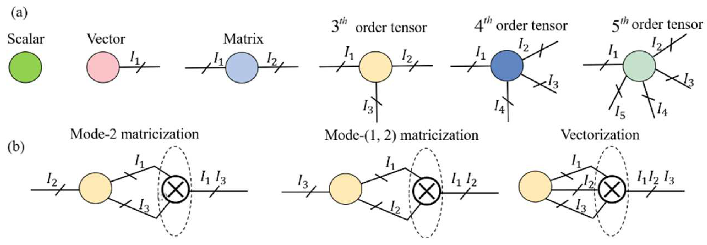
3.1. Tensor Operations
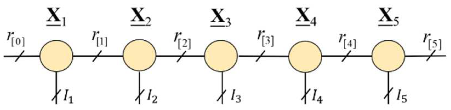
3.2. Tensor Train (TT) Decomposition
3.3. Quantum Information Theory
4. Methodology
4.1. Ability of Tensor Train in Capturing the Global Correlation
4.2. Unsupervised Tensor Train for Change Detection
| Algorithm 1. Pseudocode of the proposed UTT for multitemporal HSI change detection. |
| Input: Observed data , index set |
| Parameters: |
| Initialization: Initialize with |
| While not converged do: |
| for k = 1 to N-1 do |
| Unfold tensor to get |
| end for |
| Update tensor using Equation (22) |
| End while |
| Apply K-Means to the reconstructed tensor |
| Output: Change detection results |
4.3. Self-Supervised Tensor Train for Change Detection
5. Experiments
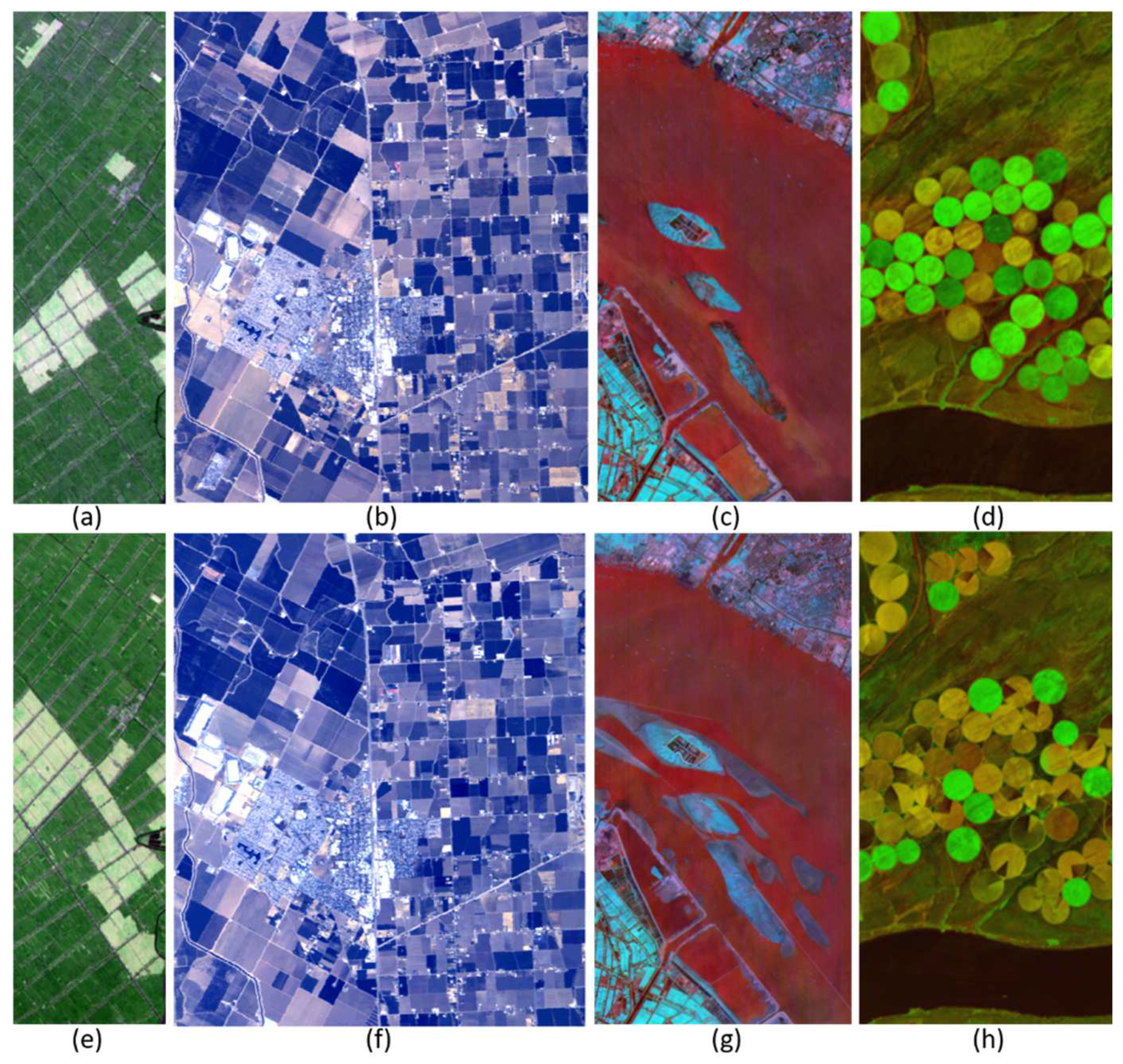
5.1. Datasets
| Algorithm 2. Pseudocode of the proposed STT for multitemporal HSI change detection. |
| Input: High-order difference tensors , pseudo-labels , maximum epochs |
| Parameters: |
| Initialization: Initialize . Maximum epochs |
| While not converged or maximum epochs not reached, do: |
| Compute and with Equations (32) and (33) |
| Update network loss L with Equation (35) |
| Update parameter set using Adam optimizer |
| Update centroids with Equation (34) |
| End while |
| Obtain features with Equation (30) |
| Perform binary clustering on |
| Output: Change detection results |
5.2. Setup
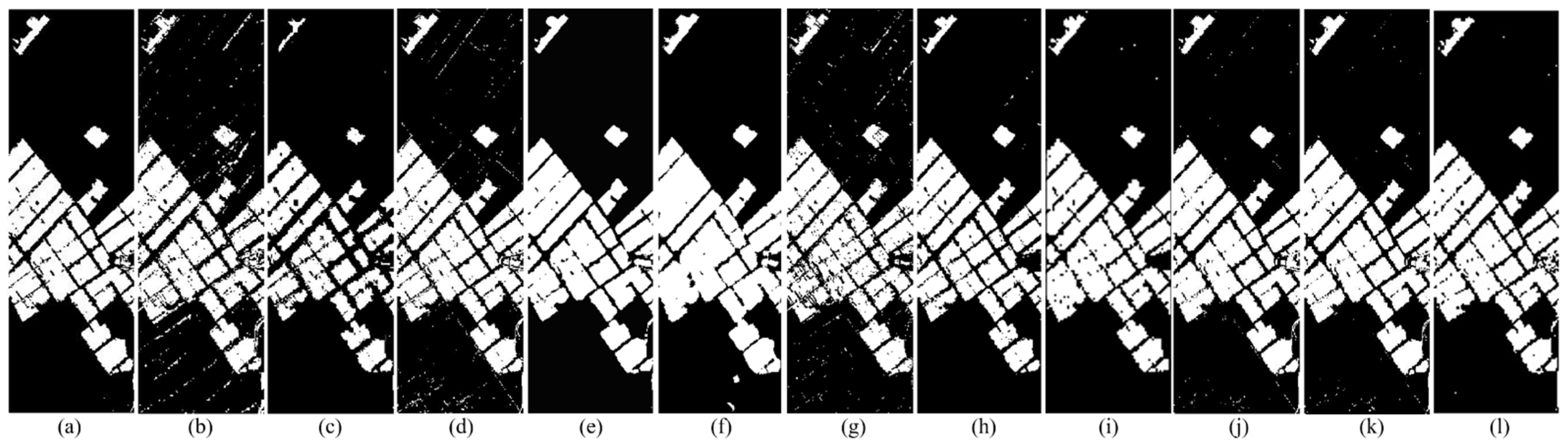
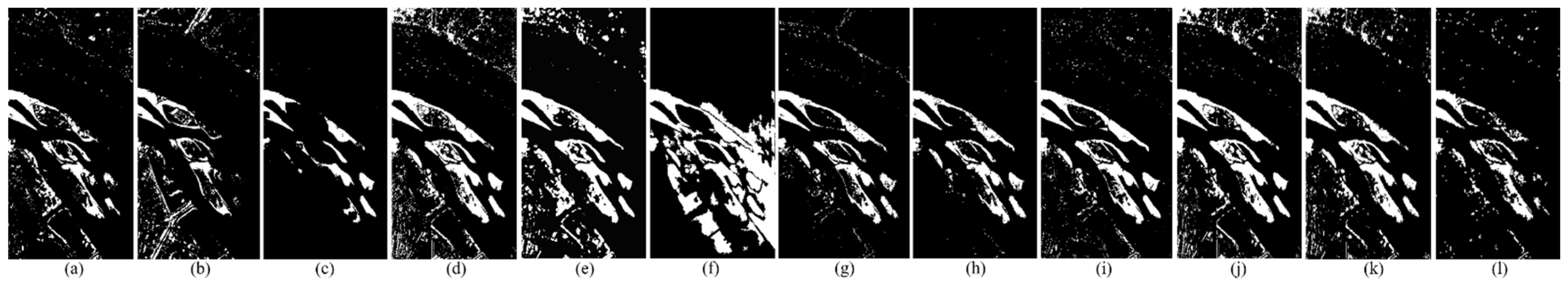
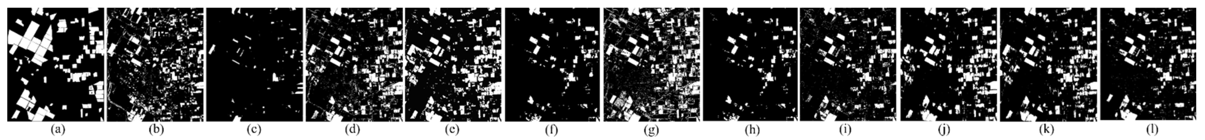
5.3. Results
5.3.1. Efficacy
5.3.2. Ablation Study
5.3.3. Efficiency
5.3.4. Discussions
- (1).
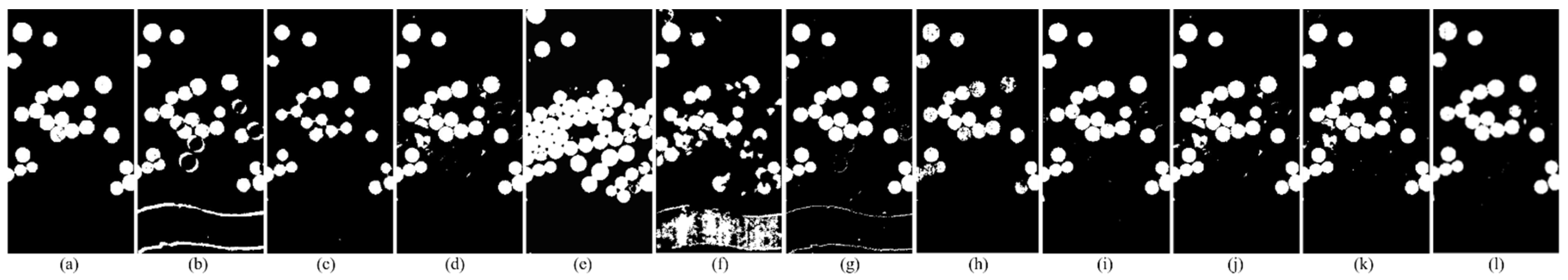
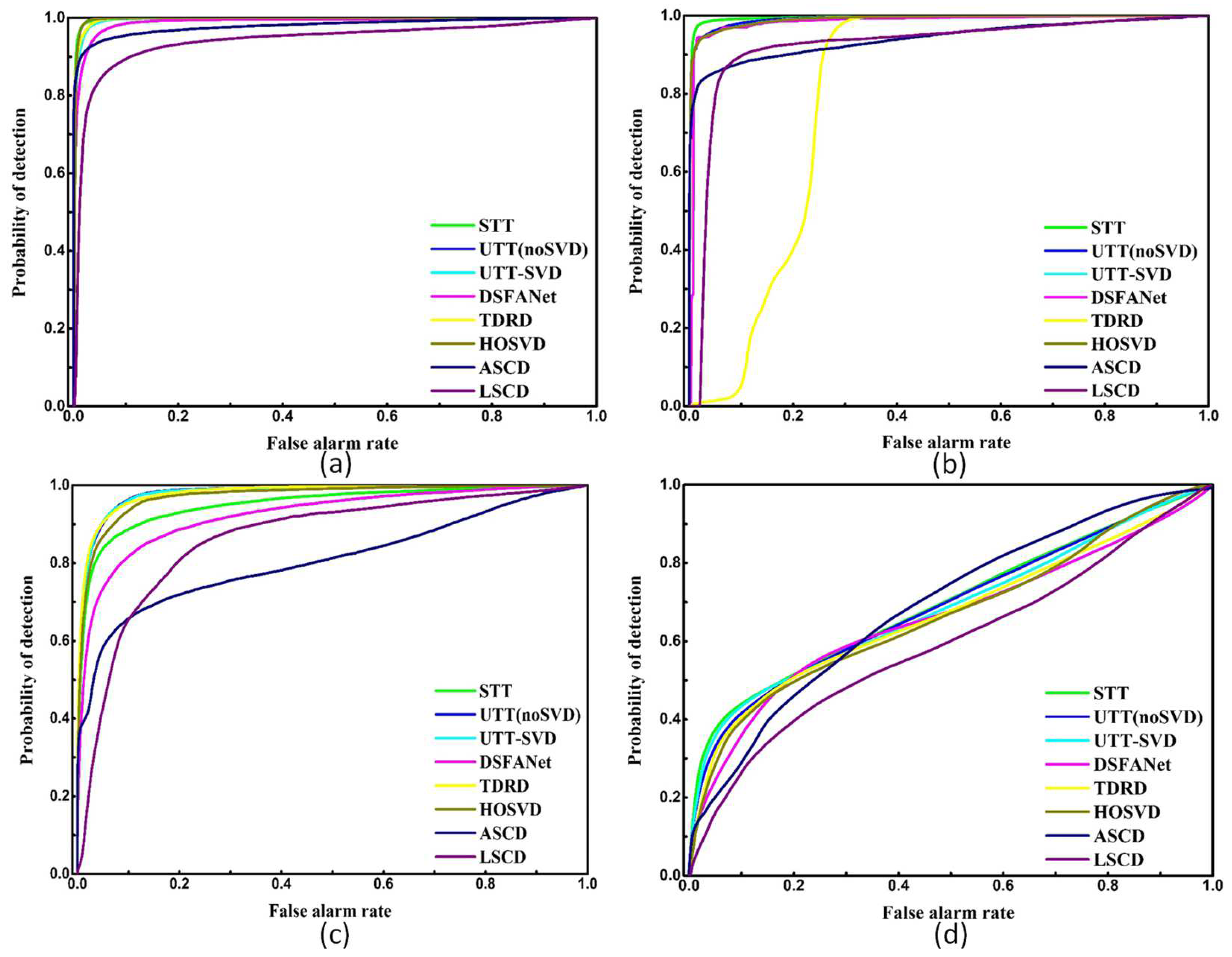
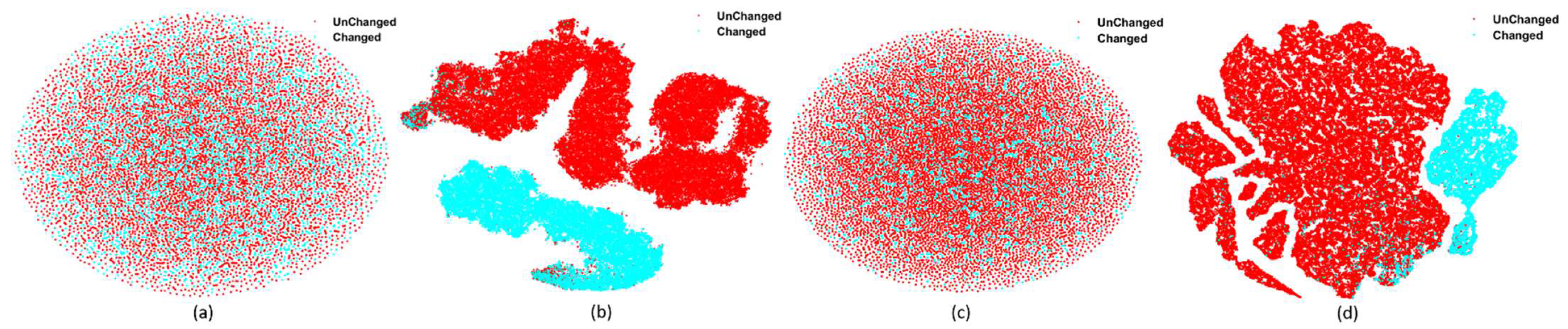
- The inter-class homogeneity and inner-class heterogeneity of HSIs are addressed by UTT and STT effectively by exploiting the ability of TT in capturing global correlations. To be specific, UTT and STT can detect changed and unchanged regions in a more balanced way due to the correlations that TT captures between the changed and unchanged information contained in the original HSIs. This can be validated by the better OA, KAPPA, and AUC values of UTT and STT as compared to the TD-based methods HOSVD [20], TDRD [18], and SSTN [38], whose low-rank features are extracted in an unbalanced way. The T-SNE results in Figure 11 also indicate that the features extracted by the TT-based methods are discriminative enough to differentiate between the changed and unchanged regions in HSI CD.
- (2).
- Both UTT and STT successfully handle the high dimensionality of HSIs by TT decomposition, which decomposes N-order weight tensors into small three-order tensor cores by approximating the low-order optimal TT ranks. Hence, the dimensionality can be reduced and the redundant information can be removed. At the same time, the execution time of UTT-noSVD is obviously lower than other existing unsupervised HSI CD methods such as LSCD [30]. Costly manual annotations can also be removed as unsupervised learning and self-learning are introduced into UTT and STT, respectively.
- (3).
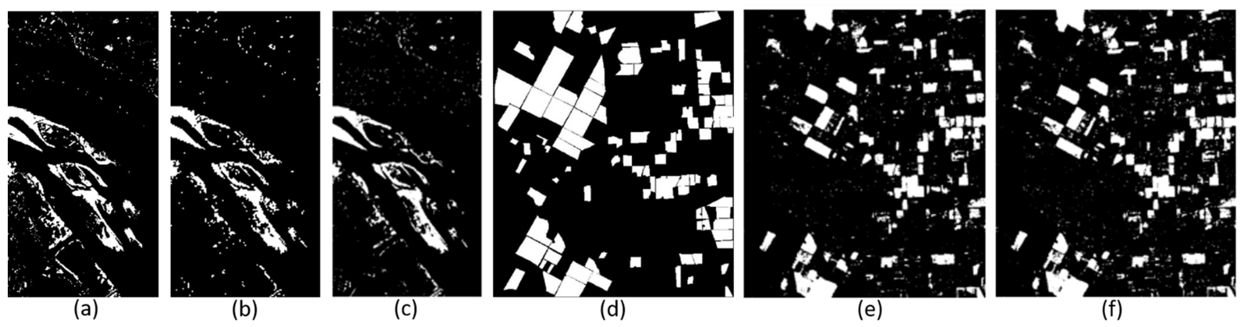
- Tensor augmentation is achieved through the KA scheme, which involves replacing a low-order tensor with a higher-order tensor without changing the number of tensor entries. Therefore, a high-order tensor with richer texture features can be achieved without increasing computation complexity. It can be seen in Figure 12 and Table 3 that KA indeed works in our proposed methods.
6. Conclusions
Author Contributions
Funding
Conflicts of Interest
References
- Bovolo, F.; Marchesi, S.; Bruzzone, L. A framework for automatic and unsupervised detection of multiple changes in multitemporal images. IEEE Trans. Geosci. Remote Sens. 2011, 50, 2196–2212. [Google Scholar] [CrossRef]
- Liu, S.; Bruzzone, L.; Bovolo, F.; Du, P. Hierarchical unsupervised change detection in multitemporal hyperspectral images. IEEE Trans. Geosci. Remote Sens. 2014, 53, 244–260. [Google Scholar]
- Deng, J.S.; Wang, K.; Deng, Y.H.; Qi, G.J. PCA based land use change detection and analysis using multitemporal and multisensor satellite data. Int. J. Remote Sens. 2008, 29, 4823–4838. [Google Scholar] [CrossRef]
- Lu, D.; Mausel, P.; Brondizio, E.; Moran, E. Change detection techniques. Int. J. Remote Sens. 2004, 25, 2365–2401. [Google Scholar] [CrossRef]
- Kennedy, R.E.; Townsend, P.A.; Gross, J.E.; Cohen, W.B.; Bolstad, P.; Wang, Y.Q.; Adams, P. Remote sensing change detection tools for natural resource managers: Understanding concepts and tradeoffs in the design of landscape monitoring projects. Remote Sens. Environ. 2009, 113, 1382–1396. [Google Scholar] [CrossRef]
- Coppin, P.R.; Bauer, M.E. Digital change detection in forest ecosystems with remote sensing imagery. Remote Sens. Rev. 1996, 13, 207–234. [Google Scholar] [CrossRef]
- Yang, X.; Chen, L. Using multi-temporal remote sensor imagery to detect earthquake-triggered landslides. Int. J. Appl. Earth Obs. Geoinf. 2010, 12, 487–495. [Google Scholar] [CrossRef]
- Ma, L.; Li, M.; Blaschke, T.; Ma, X.; Tiede, D.; Cheng, L.; Chen, Z.; Chen, D. Object-based change detection in urban areas: The effects of segmentation strategy, scale, and feature space on unsupervised methods. Remote Sens. 2016, 8, 761. [Google Scholar] [CrossRef] [Green Version]
- Hasanlou, M.; Seydi, S.T. Hyperspectral change detection: An experimental comparative study. Int. J. Remote Sens. 2018, 39, 7029–7083. [Google Scholar] [CrossRef]
- Guo, Q.; Zhang, J.; Zhong, C.; Zhang, Y. Change Detection for Hyperspectral Images via Convolutional Sparse Analysis and Temporal Spectral Unmixing. IEEE J. Sel. Top. Appl. Earth Obs. Remote Sens. 2021, 14, 4417–4426. [Google Scholar] [CrossRef]
- Wu, C.; Zhang, L.; Du, B. Kernel slow feature analysis for scene change detection. IEEE Trans. Geosci. Remote Sens. 2017, 55, 2367–2384. [Google Scholar] [CrossRef]
- Gao, F.; Dong, J.; Li, B.; Xu, Q. Automatic change detection in synthetic aperture radar images based on PCANet. IEEE Geosci. Remote Sens. Lett. 2016, 13, 1792–1796. [Google Scholar] [CrossRef]
- Chen, J.; Yuan, Z.; Peng, J.; Chen, L.; Huang, H.; Zhu, J.; Liu, Y.; Li, H. Dasnet: Dual attentive fully convolutional siamese networks for change detection of high resolution satellite images. IEEE J. Sel. Top. Appl. Earth Obs. Remote Sens. 2020, 14, 1194–1206. [Google Scholar] [CrossRef]
- Hou, B.; Liu, Q.; Wang, H.; Wang, Y. From W-Net to CDGAN: Bitemporal change detection via deep learning techniques. IEEE Trans. Geosci. Remote Sens. 2019, 58, 1790–1802. [Google Scholar] [CrossRef] [Green Version]
- Wang, Q.; Yuan, Z.; Du, Q.; Li, X. GETNET: A general end-to-end 2-D CNN framework for hyperspectral image change detection. IEEE Trans. Geosci. Remote Sens. 2018, 57, 3–13. [Google Scholar] [CrossRef] [Green Version]
- Shi, Q.; Liu, M.; Li, S.; Liu, X.; Wang, F.; Zhang, L. A Deeply Supervised Attention Metric-Based Network and an Open Aerial Image Dataset for Remote Sensing Change Detection. IEEE Trans. Geosci. Remote Sens. 2021, 60, 5604816. [Google Scholar] [CrossRef]
- Yang, B.; Fu, X.; Sidiropoulos, N.D.; Hong, M. Towards k-means-friendly spaces: Simultaneous deep learning and clustering. In Proceedings of the 34th International Conference on Machine Learning, Sydney, Australia, 6–11 August 2017; pp. 3861–3870. [Google Scholar]
- Hou, Z.; Li, W.; Tao, R.; Du, Q. Three-Order Tucker Decomposition and Reconstruction Detector for Unsupervised Hyperspectral Change Detection. IEEE J. Sel. Top. Appl. Earth Obs. Remote Sens. 2021, 14, 6194–6205. [Google Scholar] [CrossRef]
- Huang, F.; Yu, Y.; Feng, T. Hyperspectral remote sensing image change detection based on tensor and deep learning. J. Vis. Commun. Image Represent. 2019, 58, 233–244. [Google Scholar] [CrossRef]
- Chen, Z.; Wang, B.; Niu, Y.; Xia, W.; Zhang, J.Q.; Hu, B. Change detection for hyperspectral images based on tensor analysis. In Proceedings of the IEEE International Geoscience and Remote Sensing Symposium, Milan, Italy, 26–31 July 2015; pp. 1662–1665. [Google Scholar]
- Kolda, T.G.; Bader, B.W. Tensor decompositions and applications. SIAM Rev. 2009, 51, 455–500. [Google Scholar] [CrossRef]
- Cichocki, A. Era of big data processing: A new approach via tensor networks and tensor decompositions. arXiv 2014, arXiv:1403.2048. [Google Scholar]
- Nielsen, M.A.; Chuang, I. Quantum Computation and Quantum Information; Cambridge University Press: Cambridge, UK, 2002. [Google Scholar]
- Oseledets, I.V. Tensor-train decomposition. SIAM J. Sci. Comput. 2011, 33, 2295–2317. [Google Scholar] [CrossRef]
- Bengua, J.A.; Phien, H.N.; Tuan, H.D.; Do, M.N. Efficient tensor completion for color image and video recovery: Low-rank tensor train. IEEE Trans. Image Process. 2017, 26, 2466–2479. [Google Scholar] [CrossRef] [Green Version]
- Latorre, J.I. Image compression and entanglement. arXiv 2005, arXiv:quant-ph/0510031. [Google Scholar]
- Du, P.; Liu, S.; Gamba, P.; Tan, K.; Xia, J. Fusion of difference images for change detection over urban areas. IEEE J. Sel. Top. Appl. Earth Obs. Remote Sens. 2012, 5, 1076–1086. [Google Scholar] [CrossRef]
- Du, B.; Ru, L.; Wu, C.; Zhang, L. Unsupervised deep slow feature analysis for change detection in multi-temporal remote sensing images. IEEE Trans. Geosci. Remote Sens. 2019, 57, 9976–9992. [Google Scholar] [CrossRef] [Green Version]
- Li, Q.; Gong, H.; Dai, H.; Li, C.; He, Z.; Wang, W.; Mu, T. Unsupervised Hyperspectral Image Change Detection via Deep Learning Self-Generated Credible Labels. IEEE J. Sel. Top. Appl. Earth Obs. Remote Sens. 2021, 14, 9012–9024. [Google Scholar] [CrossRef]
- Wu, C.; Du, B.; Zhang, L. A subspace-based change detection method for hyperspectral images. IEEE J. Sel. Top. Appl. Earth Obs. Remote Sens. 2013, 6, 815–830. [Google Scholar] [CrossRef]
- Zhang, P.; Gong, M.; Zhang, H.; Liu, J.; Ban, Y. Unsupervised difference representation learning for detecting multiple types of changes in multitemporal remote sensing images. IEEE Trans. Geosci. Remote Sens. 2018, 57, 2277–2289. [Google Scholar] [CrossRef]
- López-Fandiño, J.; Garea, A.S.; Heras, D.B.; Arguello, F. Stacked autoencoders for multiclass change detection in hyperspectral images. In Proceedings of the IEEE International Geoscience and Remote Sensing Symposium, Valencia, Spain, 22–27 July 2018; pp. 1906–1909. [Google Scholar]
- Hou, Z.; Li, W.; Li, L.; Tao, R.; Du, Q. Hyperspectral change detection based on multiple morphological profiles. IEEE Trans. Geosci. Remote Sens. 2021, 60, 5507312. [Google Scholar] [CrossRef]
- Seydi, S.T.; Shah-Hosseini, R.; Hasanlou, M. New framework for hyperspectral change detection based on multi-level spectral unmixing. Appl. Geomat. 2021, 13, 763–780. [Google Scholar] [CrossRef]
- Seydi, S.T.; Hasanlou, M. A New Structure for Binary and Multiple Hyperspectral Change Detection Based on Spectral Unmixing and Convolutional Neural Network. Measurement 2021, 186, 110137. [Google Scholar] [CrossRef]
- Hasanlou, M.; Seydi, S.T.; Shah-Hosseini, R. A sub-pixel multiple change detection approach for hyperspectral imagery. Can. J. Remote Sens. 2018, 44, 601–615. [Google Scholar] [CrossRef]
- Jafarzadeh, H.; Hasanlou, M. An unsupervised binary and multiple change detection approach for hyperspectral imagery based on spectral unmixing. IEEE J. Sel. Top. Appl. Earth Obs. Remote Sens. 2019, 12, 4888–4906. [Google Scholar] [CrossRef]
- Zhou, F.; Chen, Z. Hyperspectral Image Change Detection by Self-Supervised Tensor Network. In Proceedings of the IEEE International Geoscience and Remote Sensing Symposium, Waikoloa, HI, USA, 19–24 July 2020; pp. 2527–2530. [Google Scholar]
- Zhang, R.; Isola, P.; Efros, A.A. Colorful image colorization. In Proceedings of the European Conference on Computer Vision, Amsterdam, The Netherlands, 11–14 October 2016; pp. 649–666. [Google Scholar]
- Pathak, D.; Krahenbuhl, P.; Donahue, J.; Darrell, T.; Efros, A.A. Context encoders: Feature learning by inpainting. In Proceedings of the IEEE conference on computer vision and pattern recognition, Las Vegas, NV, USA, 27–30 June 2016; pp. 2536–2544. [Google Scholar]
- Noroozi, M.; Favaro, P. Unsupervised learning of visual representations by solving jigsaw puzzles. In Proceedings of the European Conference on Computer Vision, Amsterdam, The Netherlands, 11–14 October 2016; pp. 69–84. [Google Scholar]
- Long, J.; Shelhamer, E.; Darrell, T. Fully convolutional networks for semantic segmentation. In Proceedings of the IEEE Conference on Computer Vision and Pattern Recognition, Boston, MA, USA, 7–12 June 2015; pp. 3431–3440. [Google Scholar]
- Girshick, R.; Donahue, J.; Darrell, T.; Malik, J. Rich feature hierarchies for accurate object detection and semantic segmentation. In Proceedings of the IEEE Conference on Computer Vision and Pattern Recognition, Columbus, OH, USA, 23–28 June 2014; pp. 580–587. [Google Scholar]
- Dong, H.; Ma, W.; Jiao, L.; Liu, F.; Li, L. A Multiscale Self-Attention Deep Clustering for Change Detection in SAR Images. IEEE Trans. Geosci. Remote Sens. 2021, 60, 1–16. [Google Scholar] [CrossRef]
- Chen, Y.; Bruzzone, L. Self-supervised Change Detection in Multi-view Remote Sensing Images. arXiv 2021, arXiv:2103.05969. [Google Scholar]
- Deng, Y.J.; Li, H.C.; Fu, K.; Du, Q.; Emery, W.J. Tensor low-rank discriminant embedding for hyperspectral image dimensionality reduction. IEEE Trans. Geosci. Remote Sens. 2018, 56, 7183–7194. [Google Scholar] [CrossRef]
- Zhao, M.; Li, W.; Li, L.; Ma, P.; Tao, R. Three-order tensor creation and tucker decomposition for infrared small-target detection. IEEE Trans. Geosci. Remote Sens. 2021, 99, 1–16. [Google Scholar] [CrossRef]
- Li, L.; Li, W.; Qu, Y.; Zhao, C.; Tao, R.; Du, Q. Prior-based tensor approximation for anomaly detection in hyperspectral imagery. IEEE Trans. Neural Netw. Learn. Syst. 2020, 33, 1037–1050. [Google Scholar] [CrossRef]
- Velasco-Forero, S.; Angulo, J. Classification of hyperspectral images by tensor modeling and additive morphological decomposition. Pattern Recognit. 2013, 46, 566–577. [Google Scholar] [CrossRef] [Green Version]
- Zniyed, Y. Breaking the Curse of Dimensionality Based on Tensor Train: Models and Algorithms. Ph.D. Thesis, Paris-Saclay, Paris, France, 2019. [Google Scholar]
- Henderson, L.; Vedral, V. Classical, quantum and total correlations. J. Phys. A. Math. Gen. 2001, 34, 6899–6905. [Google Scholar] [CrossRef]
- Novikov, A.; Podoprikhin, D.; Osokin, A.; Vetrov, D. Tensorizing neural network. arXiv 2015, arXiv:1509.06569. [Google Scholar]
- Kingma, D.P.; Ba, J. Adam: A method for stochastic optimization. arXiv 2014, arXiv:1412.6980. [Google Scholar]
- López-Fandiño, J.; B Heras, D.; Arguello, F.; Dalla, M.M. GPU framework for change detection in multitemporal hyperspectral images. Int. J. Parallel Program. 2019, 47, 272–292. [Google Scholar] [CrossRef]
- Perez-Garcia, D.; Verstraete, F.; Wolf, M.M.; Cirac, J.I. Matrix product state representations. arXiv 2006, arXiv:quant-ph/0608197. [Google Scholar] [CrossRef]


| Data Set | Metric | LS CD | AS CD | HO SVD | TD RD | PCA- Net | DSFA-Net | HI- DRL | SSTN | UTT-SVD | UTT-noSVD | STT |
|---|---|---|---|---|---|---|---|---|---|---|---|---|
| Yancheng | CA_UN(%) | 94.33 | 99.94 | 97.79 | 95.67 | 94.11 | 97.01 | 99.10 | 98.19 | 98.17 | 98.15 | 97.79 |
| CA_CH(%) | 85.13 | 75.89 | 98.69 | 95.09 | 98.35 | 92.40 | 92.00 | 96.25 | 97.78 | 98.03 | 98.69 | |
| OA(%) | 91.73 | 93.13 | 98.04 | 97.31 | 95.31 | 95.71 | 97.09 | 97.64 | 98.07 | 98.11 | 98.20 | |
| KAPPA | 0.7959 | 0.8176 | 0.9524 | 0.9345 | 0.8890 | 0.8942 | 0.9270 | 0.9420 | 0.9528 | 0.9536 | 0.9561 | |
| River | CA_UN(%) | 92.71 | 97.92 | 92.37 | 92.03 | 83.17 | 97.06 | 98.76 | 97.34 | 92.16 | 93.71 | 98.44 |
| CA_CH(%) | 44.13 | 40.32 | 90.72 | 94.03 | 68.55 | 66.21 | 58.48 | 72.84 | 91.01 | 85.95 | 69.24 | |
| OA(%) | 88.48 | 92.93 | 92.23 | 92.21 | 81.52 | 94.25 | 94.23 | 94.58 | 92.30 | 93.10 | 95.90 | |
| KAPPA | 0.3364 | 0.4768 | 0.6283 | 0.6365 | 0.3590 | 0.6768 | 0.6640 | 0.7210 | 0.6285 | 0.6462 | 0.7237 | |
| Bay Area | CA_UN(%) | 86.90 | 99.54 | 87.30 | 85.96 | 89.36 | 82.19 | 97.59 | 93.17 | 90.72 | 91.81 | 94.29 |
| CA_CH(%) | 31.44 | 11.02 | 42.96 | 45.28 | 38.50 | 48.64 | 25.02 | 36.60 | 42.73 | 39.54 | 38.72 | |
| OA(%) | 73.32 | 77.86 | 76.44 | 75.37 | 78.23 | 73.97 | 81.71 | 80.79 | 78.97 | 78.98 | 81.02 | |
| KAPPA | 0.2028 | 0.1500 | 0.3220 | 0.3006 | 0.3040 | 0.3046 | 0.2970 | 0.3460 | 0.3708 | 0.3652 | 0.3841 | |
| Hermiston | CA_UN(%) | 94.77 | 99.74 | 98.14 | 76.82 | 85.48 | 98.76 | 99.76 | 99.33 | 98.20 | 98.48 | 99.02 |
| CA_CH(%) | 80.88 | 70.13 | 93.36 | 55.55 | 67.78 | 91.35 | 83.86 | 93.88 | 93.29 | 92.95 | 95.02 | |
| OA(%) | 92.99 | 95.95 | 97.53 | 74.09 | 83.19 | 97.81 | 97.72 | 98.63 | 97.57 | 97.76 | 98.83 | |
| KAPPA | 0.7068 | 0.7938 | 0.8922 | 0.2181 | 0.4140 | 0.9018 | 0.8910 | 0.9380 | 0.8936 | 0.9010 | 0.9384 |
| Methods | Yancheng | Hermiston | River | Bay Area |
|---|---|---|---|---|
| LSCD | 0.9400 | 0.9224 | 0.8629 | 0.5968 |
| ASCD | 0.9796 | 0.9420 | 0.8082 | 0.6927 |
| HOSVD | 0.9960 | 0.9908 | 0.9719 | 0.6685 |
| TDRD | 0.9968 | 0.8022 | 0.9807 | 0.6699 |
| DSFANet | 0.9887 | 0.9841 | 0.9273 | 0.6595 |
| UTT-SVD | 0.9964 | 0.9910 | 0.9813 | 0.6863 |
| UTT-noSVD | 0.9967 | 0.9919 | 0.9817 | 0.6907 |
| STT | 0.9970 | 0.9951 | 0.9531 | 0.6978 |
| Methods | River | Bay Area | ||
|---|---|---|---|---|
| OA (%) | KAPPA | OA (%) | KAPPA | |
| STT(3-Dimensional) | 95.62 | 0.7080 | 80.36 | 0.3820 |
| STT(5-Dimensional) | 95.90 | 0.7237 | 81.02 | 0.3841 |
| Methods | Yancheng | Bay Area | River | Hermiston |
|---|---|---|---|---|
| LSCD | 3.945 | 217.662 | 38.804 | 18.838 |
| ASCD | 3.866 | 129.609 | 20.487 | 7.421 |
| HOSVD | 4.908 | 43.480 | 11.830 | 9.316 |
| UTT-SVD | 8.992 | 262.747 | 5.709 | 21.018 |
| UTT-noSVD | 1.476 | 5.441 | 0.934 | 0.678 |
Publisher’s Note: MDPI stays neutral with regard to jurisdictional claims in published maps and institutional affiliations. |
© 2022 by the authors. Licensee MDPI, Basel, Switzerland. This article is an open access article distributed under the terms and conditions of the Creative Commons Attribution (CC BY) license (https://creativecommons.org/licenses/by/4.0/).
Share and Cite
Sohail, M.; Wu, H.; Chen, Z.; Liu, G. Unsupervised and Self-Supervised Tensor Train for Change Detection in Multitemporal Hyperspectral Images. Electronics 2022, 11, 1486. https://doi.org/10.3390/electronics11091486
Sohail M, Wu H, Chen Z, Liu G. Unsupervised and Self-Supervised Tensor Train for Change Detection in Multitemporal Hyperspectral Images. Electronics. 2022; 11(9):1486. https://doi.org/10.3390/electronics11091486
Chicago/Turabian StyleSohail, Muhammad, Haonan Wu, Zhao Chen, and Guohua Liu. 2022. "Unsupervised and Self-Supervised Tensor Train for Change Detection in Multitemporal Hyperspectral Images" Electronics 11, no. 9: 1486. https://doi.org/10.3390/electronics11091486
APA StyleSohail, M., Wu, H., Chen, Z., & Liu, G. (2022). Unsupervised and Self-Supervised Tensor Train for Change Detection in Multitemporal Hyperspectral Images. Electronics, 11(9), 1486. https://doi.org/10.3390/electronics11091486