Constant Power Load Stabilization in DC Microgrids Using Continuous-Time Model Predictive Control

Abstract

Despite its advantages over its AC counterparts, DC microgrids present a lot of challenges. One of these challenges is the instability issues caused by constant power loads (CPLs). CPLs deteriorate the system’s performance due to their incremental negative impedance characteristics. In this paper, a DC microgrid composed of a PV/battery system feeding a pure CPL was considered. A continuous-time model predictive control combined with a disturbance observer was applied to the DC–DC bidirectional converter. The purpose of the composite controller is to address the nonlinearity of the CPL and to maintain the stability of the system in a large operating region under load and PV generation variations. To show the performance of the system, several tests were performed under PV power and CPL power variations. Simulation results show good performance in terms of transient response, optimal tracking, and stability in a large operating region.

1. Introduction

Renewable energy sources (RESs) are becoming a key solution to face the increasing demand of electricity and the environmental impact caused using fossil fuels. Photovoltaic (PV) technology is widely used in various applications due to its ease of installation, competitive cost, and wide selection [1,2]. In grid-connected applications, the excess power can be injected into the main grid, while in stand-alone applications, the use of energy storage systems (ESSs) is crucial due to the intermittent nature of PV power [3]. Hence, ESSs are used to store surplus energy for further usage to meet the load demand [4,5,6].

The integration of distributed generators, loads, and ESSs into single entities called microgrids (MGs) is conspicuously becoming more popular, especially in remote zones. For instance, PV power is used to supply telecommunication towers that are installed in remote areas [7]. Therefore, seamless control of power electronic converters is highly desired to ensure reliable and high-quality power for such systems. Generally, in a typical stand-alone PV/battery system, a DC–DC power converter is used to link the PV module to a common DC bus [8,9]. This converter is a crucial element that ensures a maximum delivery of power by the PV generator. In addition, a DC–DC bidirectional converter (BDC) is usually considered to interface the battery to the DC bus. It performs DC bus voltage regulation and battery charging/discharging operations.

Various research efforts have been devoted to cover stand-alone DC microgrids with PV/battery systems. Some researchers are predominantly focused on developing efficient maximum power point tracking (MPPT) algorithms to take advantage of the maximum ability of the PV generator [10,11,12]. This area is well studied and a lot of MPPT algorithms have been developed. For instance, conventional algorithms, such as perturb and observe and incremental conductance, are widely used due to their simplicity and satisfactory performance [13]. Additionally, high performance MPPT techniques that use artificial intelligence have been developed, such as fuzzy logic and artificial neural network [14]. Other researchers are mainly interested in the design of local controllers to improve the dynamics and the stability (e.g., [15,16]). Furthermore, many works focused more on the coordination of multiple units, the power flow management in the system, and the implementation of energy management systems, such as the works presented in [17,18,19,20].

Generally, the control of DC–DC converters in a PV/battery system is performed using cascaded control loops with proportional integral (PI) controllers. In the case of BDC, the inner loop is used to regulate the battery current to follow the reference given by the outer loop. This later maintains the DC bus voltage at a desired value. Those cascaded control loops are simple from the design and implementation point of view. However, they suffer from slow transient response and high oscillations in the steady-state [21]. PI controllers are usually tuned based on a linearized model of the system around an equilibrium point, raising concerns about stability issues in a large signal sense. Moreover, connecting a constant power load (CPL) can deteriorate the system’s performance or even lead to instability. In fact, power electronic loads when tightly controlled behave as CPLs, such as DC–DC converters feeding resistive loads [22]. This type of load implies incremental negative impedance (INI), which has a destabilizing effect on the system. The destabilizing effect of CPLs has been analyzed in various works [22,23]. In addition to the nonlinearity of CPLs, PV arrays influence the stability of the system due to their nonlinear characteristics [24].

The mitigation of instability issues caused by the nonlinearity nature of CPLs has been reported in the literature under three main approaches: passive approaches, active approaches, and advanced control techniques. The simplest way to stabilize CPLs is by adding passive components to the input filter of the system, such as resistors, inductors, and capacitors. Thus, the size, the cost, and power loss are significantly increased. For instance, the authors in [25] presented a passive damping approach by considering three different passive methods: RC parallel damping, RL parallel damping, and RL series damping. The second approach is known as the active damping method. It consists of adjusting control loops by introducing a virtual component. The main advantage of this technique is reducing the number of the components of the system, resulting in higher reliability and efficiency [26]. Since most active damping methods are based on linearized models, they can only guarantee stability in a limited operating region. To overcome this issue, the authors in [27] presented a nonlinear active damping method using the loop-cancellation technique. Advanced control techniques are also used to relieve the instability effect of CPLs [22]. A nonlinear controller based on a robust sliding mode control approach is developed in [28]. The nonlinear controller is applied to a DC microgrid with CPLs aiming to ensure the stability of the system in a wide operating region. In [24], a passivity-based controller was applied to a PV/battery system. The designed controller was able to guarantee the stability of the system under various changes of PV power and CPL power. The authors in [29] proposed a backstepping algorithm combined with a nonlinear disturbance observer to control a DC–DC boost converter feeding CPL. The resulting controller ensures large signal stability with fast dynamics and accurate voltage regulation.

As an advanced control technique, model predictive control (MPC) is well suited for the control of power converters in DC microgrids [22]. It is a powerful technique to solve optimal tracking problems. However, MPC relies on the use of an optimal model of the system to achieve the desired tracking performance, which is affected by the presence of disturbances and model uncertainties. To deal with unknown parts of the model and external disturbances, a disturbance observer can be combined with MPC to attain the desired performance. In [30], the authors proposed a composite controller based on MPC to control a DC–DC buck converter feeding a CPL. The composite controller combines MPC with a higher-order sliding mode observer to estimate disturbances and uncertainties. A Takagi–Sugeno fuzzy-based MPC was used to stabilize a DC microgrid with time-varying CPL in [31]. The authors in [32] presented an explicit MPC to mitigate the destabilizing effect of CPL. Unlike previous methods, this method does not use any disturbance observer.

The work presented in this paper presents a continuous-time model predictive controller based on the design strategy proposed in [33] for both the DC–DC boost converter and the DC–DC bidirectional converter. The continuous-time MPC controller was combined with a disturbance observer to deal with the unknown quantities. In [33], the continuous-time MPC controller was applied to a grid connected three phase PV system, and a PV/battery system with CPL was not considered in the study. The work presented in this paper focuses on CPL stabilization in DC microgrids using continuous-time MPC. In summary, the main contributions of this work are:

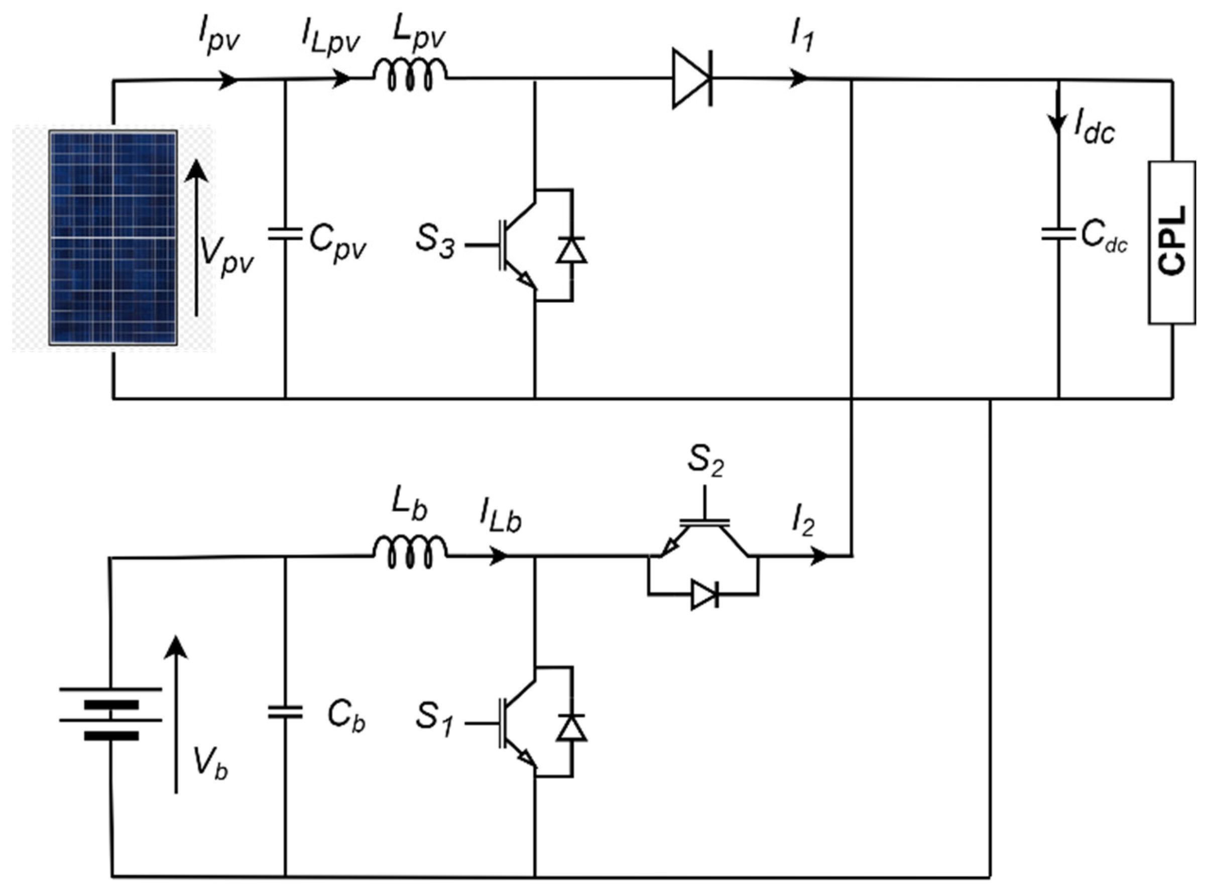
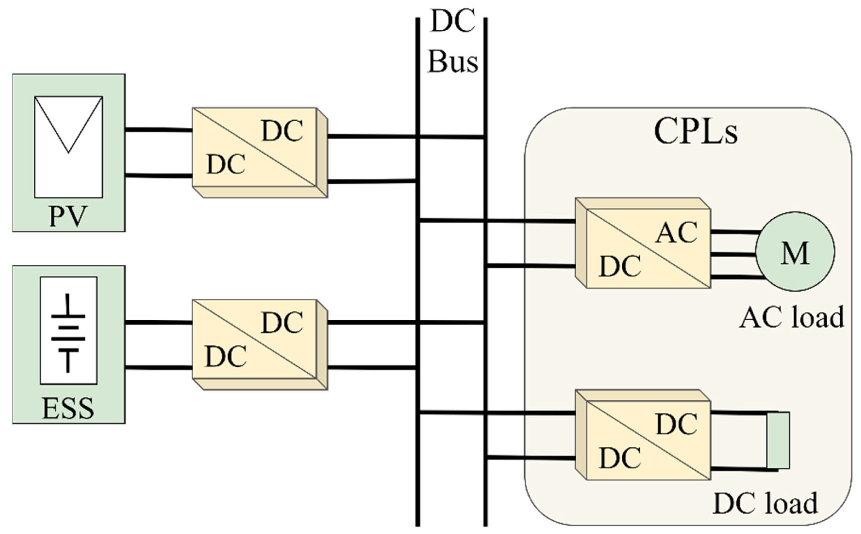
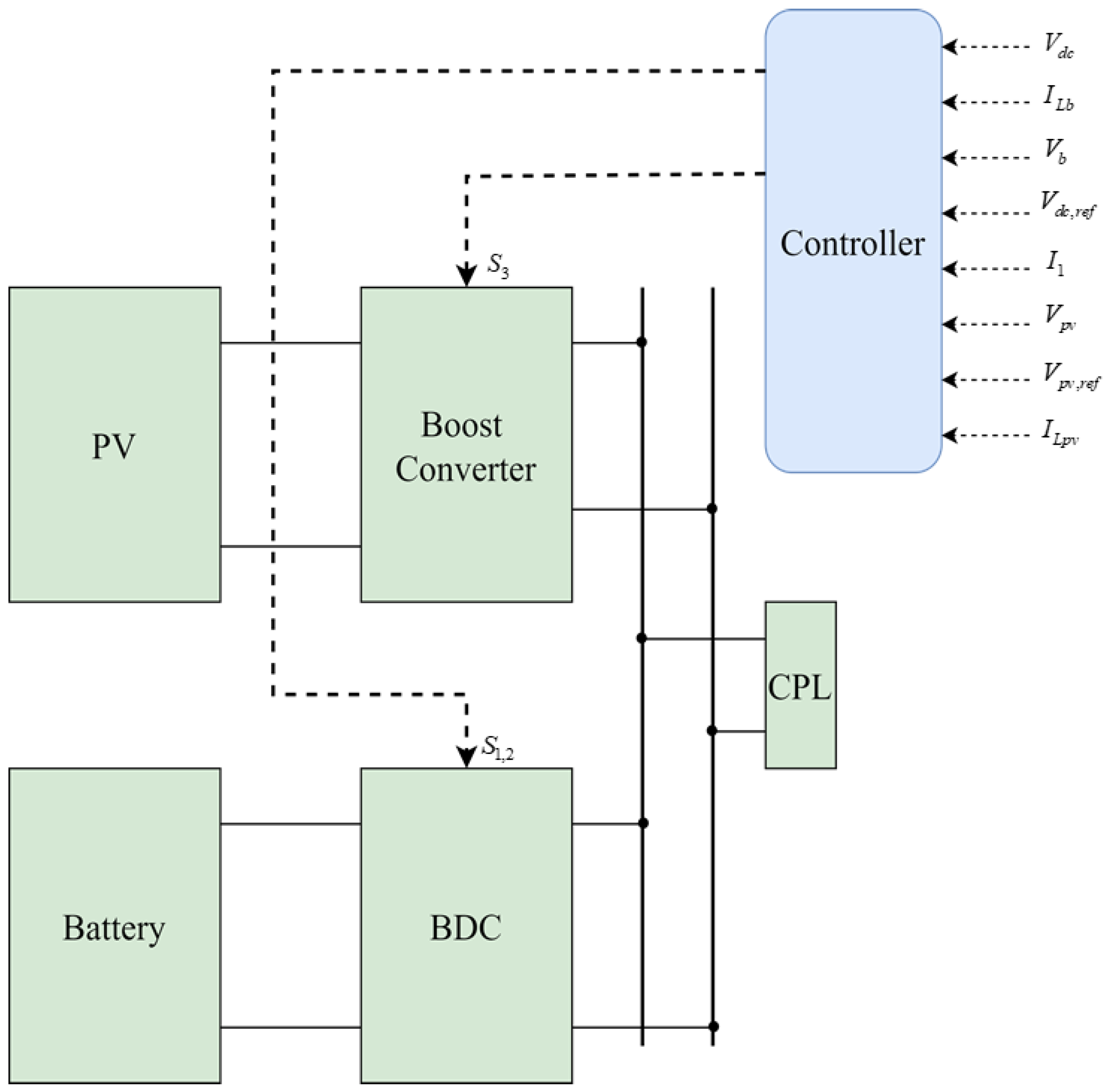
• A complete modeling of a typical DC microgrid consisting of a PV array and a battery feeding a CPL.
• Mitigation of the instability issue caused by CPL using a continuous-time MPC, which ensures accurate tracking and large signal stability.
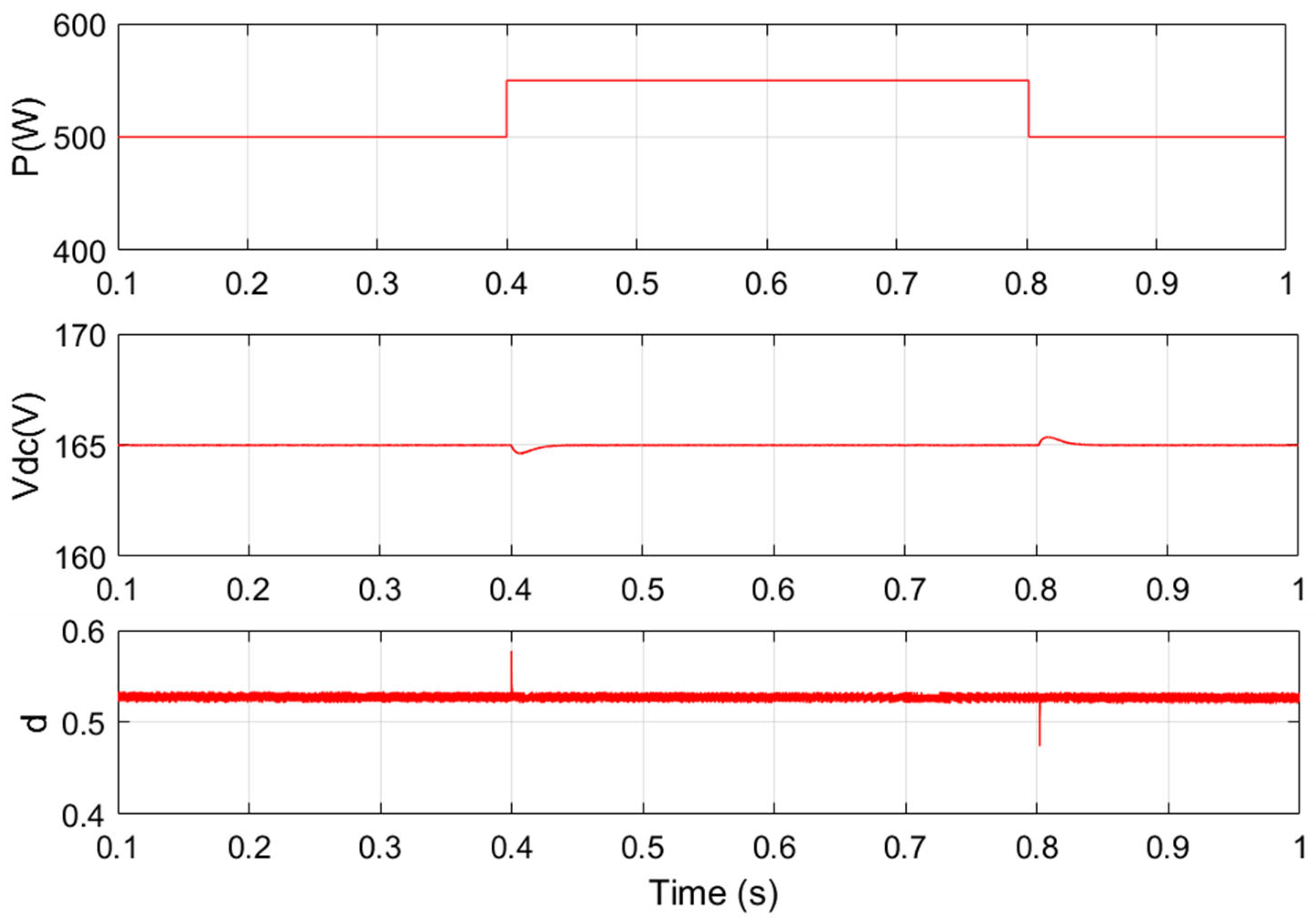
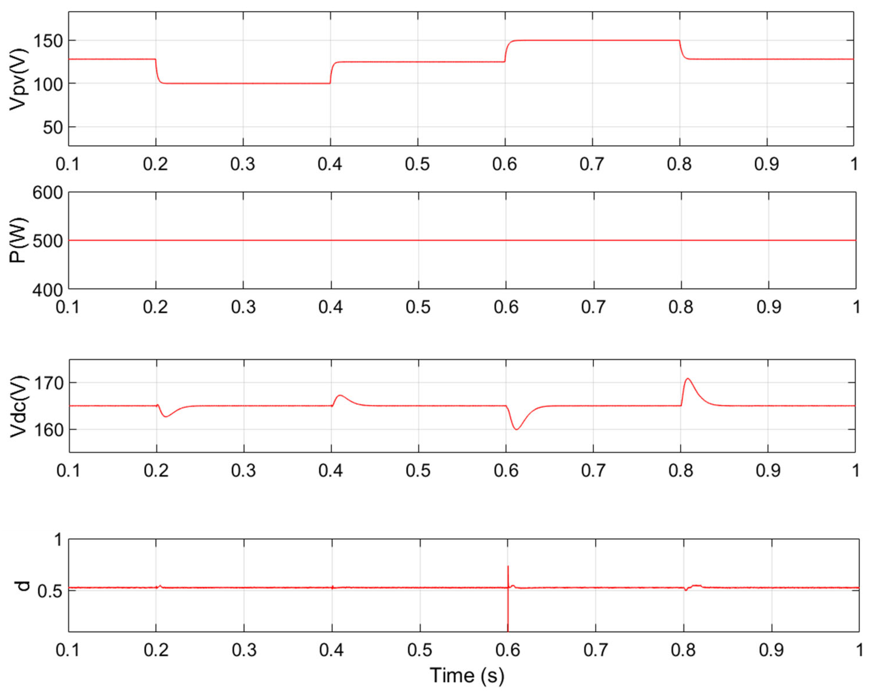
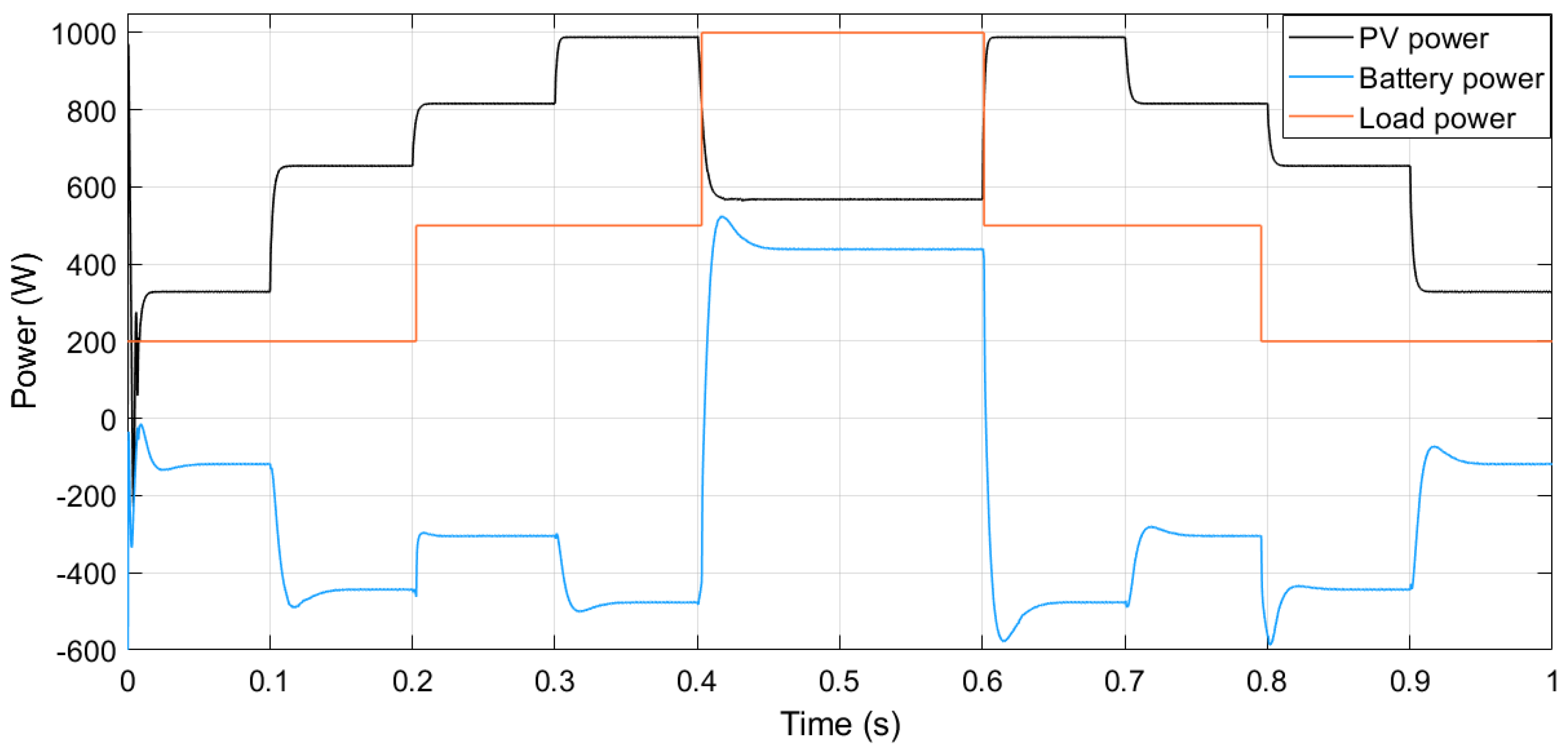
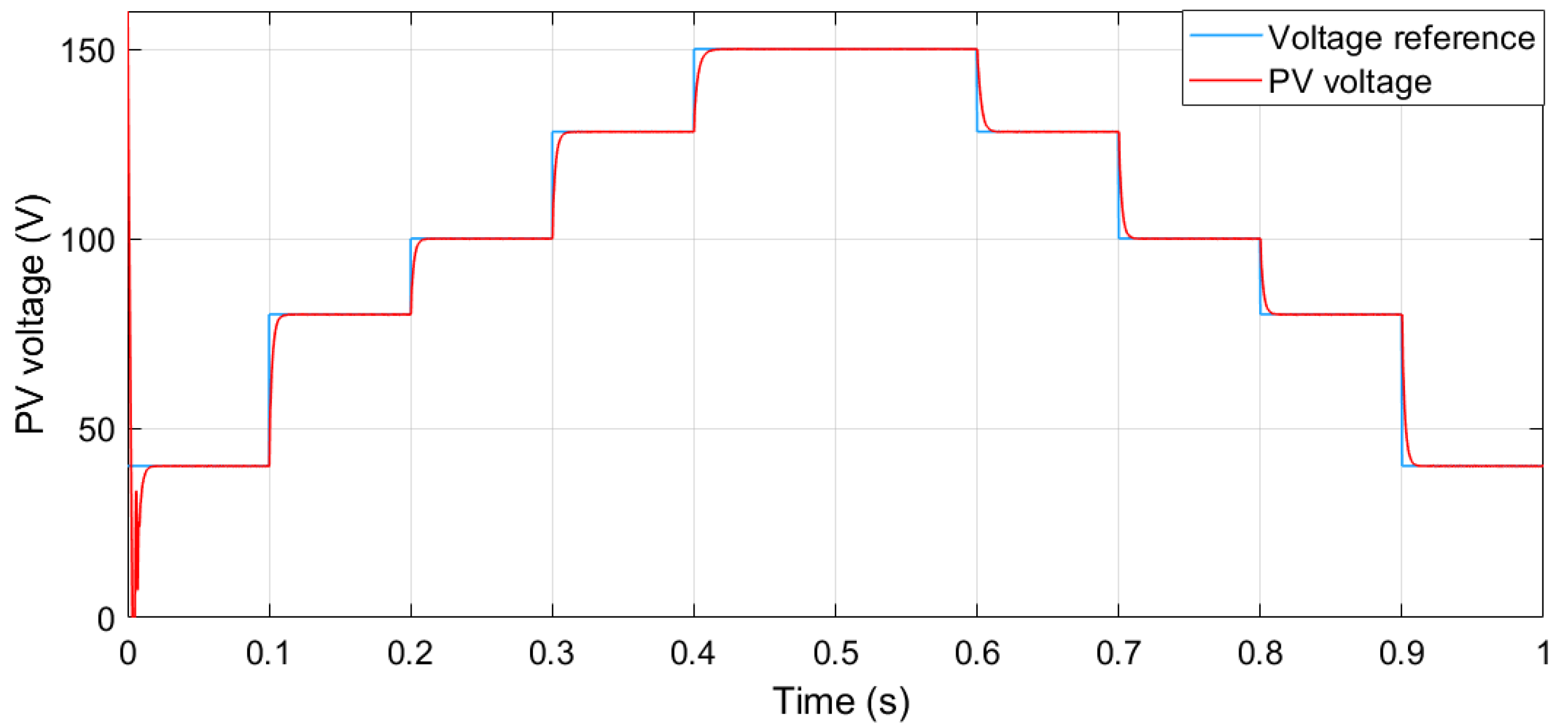
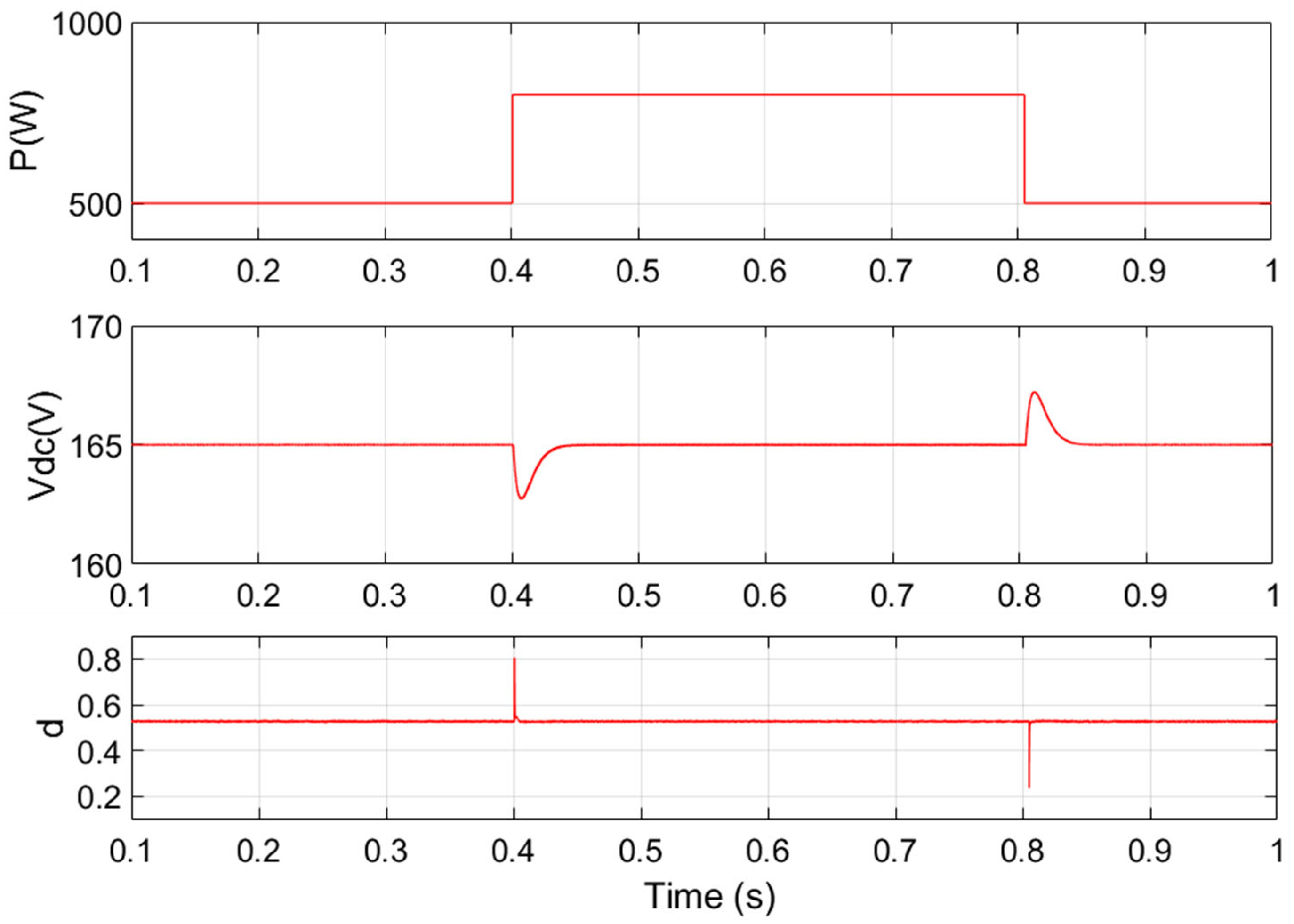
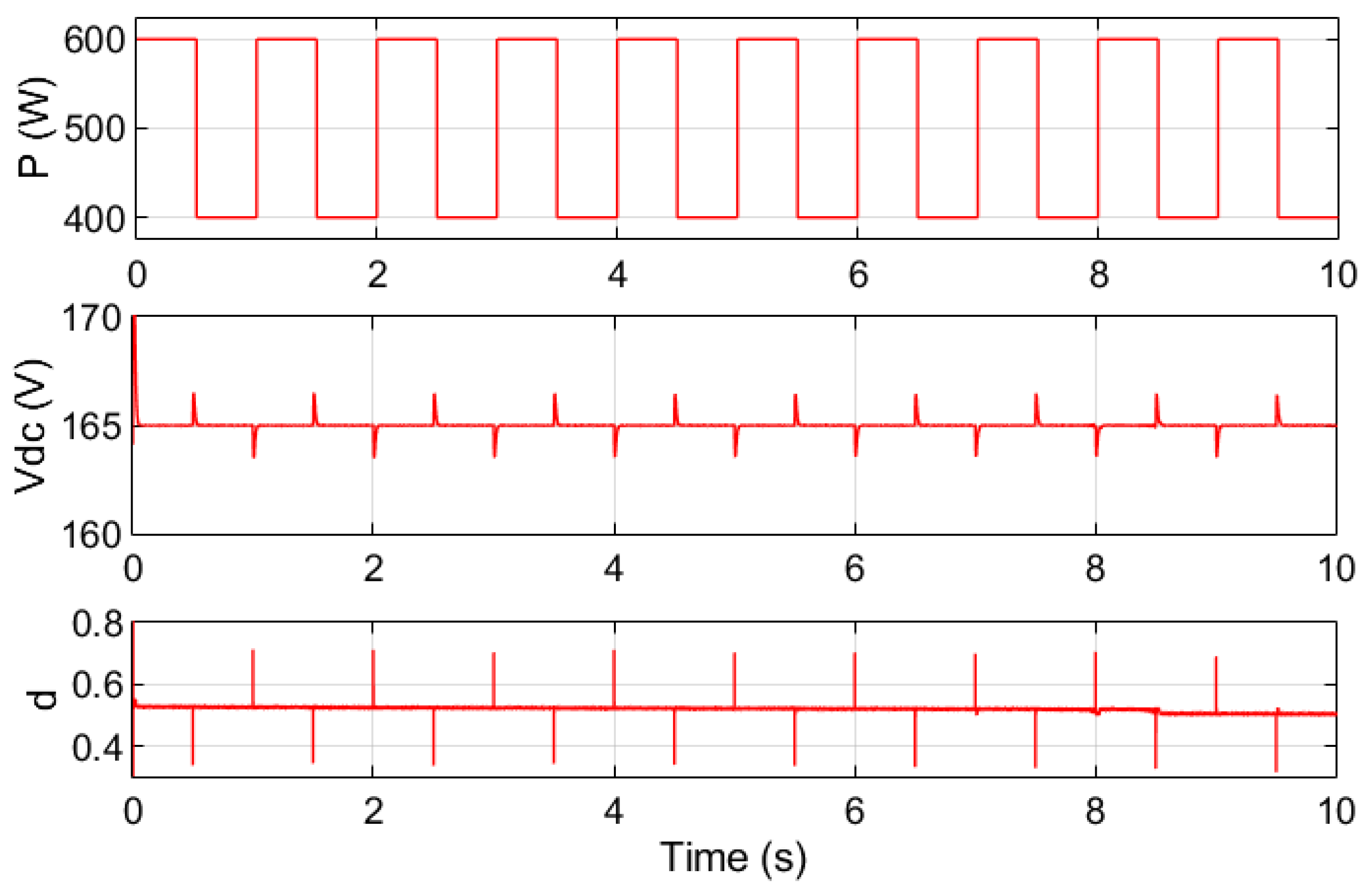
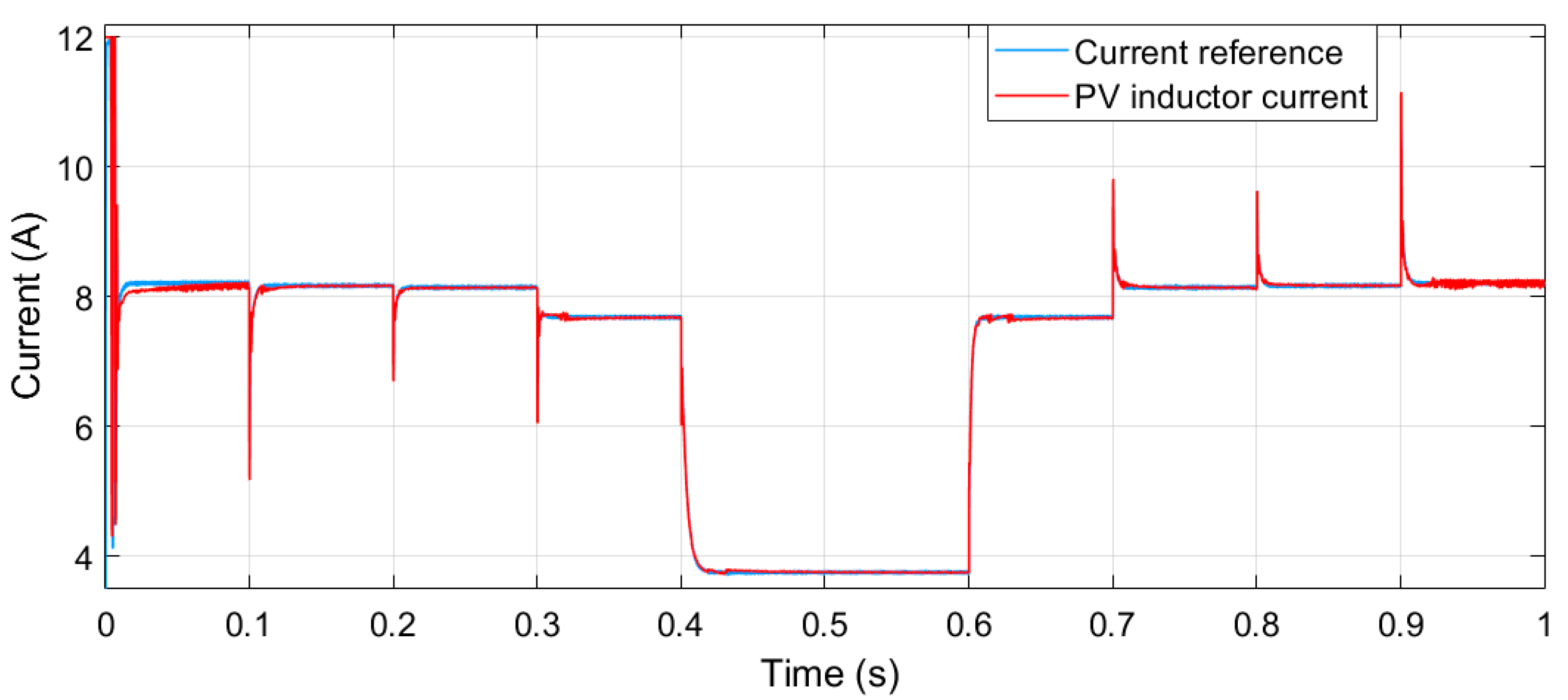
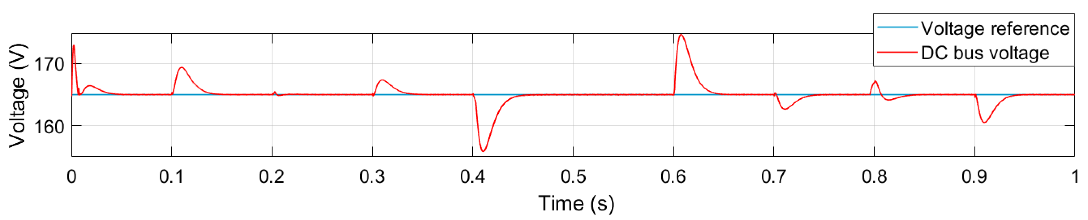
• Extensive simulations were conducted to investigate the influence of CPL on DC microgrid stability following four scenarios—small CPL power variation, large CPL variation, PV power variation, and square wave variation of the CPL.

The remainder of this paper is organized as follows. The problem formulation and system modeling are described in Section 2. Section 3 introduces the continuous-time MPC controller for a DC–DC converter in MGs. Simulation results are presented in Section 4. Finally, conclusions and perspectives are drawn in Section 5.

2. Problem Formulation and System Modeling

2.1. Problem Formulation

The majority of existing loads in DC microgrids are powered through point-of-load converters [34], as depicted in Figure 1. These converters when tightly controlled tend to draw a constant power. For instance, an inverter driving a motor with a rotating load. The motor will have a one-to-one torque–speed characteristic. Because of this linear characteristic between the speed and torque, when the motor speed is tightly controlled under constant torque, the power delivered to the motor remains constant. A CPL can then be modeled as

$$i_{CPL}=\frac{P_{CPL}}{v_{dc}}$$

(1)

where $i_{CPL}$ is the instantaneous current drawn by the CPL, $v_{dc}$ is the instantaneous DC bus voltage, and $P_{CPL}$ represents the CPL power. As can be observed, a CPL can be modeled using an ideal current source. The relation between the voltage and current of a CPL can be expressed as [23]

$$r=\frac{d{v}_{dc}}{d{i}_{CPL}}=-\frac{P_{CPL}}{i_{CPL}^2}=-\frac{v_{dc}}{i_{CPL}}$$

(2)

As can be seen from the Equation (2), the CPL presents an incremental negative impedance, which has a destabilizing effect on the system in the presence of other power converters.

2.2. System Modeling

As stated above, a typical DC microgrid is considered in the present study. The schematic of the overall studied system is depicted in Figure 2. It consists of a PV system and a battery bank. The PV system is made of a PV array and a boost converter. The battery bank is connected to the common bus through a DC–DC bidirectional converter. The two converters are connected to a DC bus through a capacitor $C_{dc}$ and feeding a CPL.

2.2.1. PV Modeling

The PV array is modeled using a single diode model with parallel resistance $R_p$ and series resistance $R_s$. The PV output current $i_{pv}$ of a PV module composed of $N_s$ cells in series can be expressed by

$$i_{pv}=I_{ph}-I_0\left(\exp \left(\frac{v_{pv}+R_s{i}_{pv}}{V_{t}a{N}_s}\right)-1\right)-\left(\frac{v_{pv}+R_s{i}_{pv}}{R_p}\right)$$

(3)

where $v_{pv}$ represents the output voltage of the PV array, $I_0$ denotes the saturation current of the diode and depends mainly on the temperature, $I_{ph}$ is the photocurrent and depends on the insolation, $V_t$ is the thermal voltage, and $a$ denotes the ideality factor of the diode. This model is validated experimentally in the EEBLab (Energy Efficient Building Laboratory) in our university [35].

2.2.2. Battery Modeling

The battery is modeled using a controlled voltage source $E_{bat}$ in series with internal resistor $R_i$. The internal resistor is assumed to be constant, and the effect of the temperature is neglected. Considering a battery with a capacity $Q$, the battery voltage $V_{bat}$ for the charging mode and discharging mode can be described respectively as follows [36]:

$$V_{bat}=E_{bat}-R_i·i=E_0-R_i·i-\lambda \frac{Q}{Q-it}(it+i^{*})+Exp(t)$$

(4)

$$V_{bat}=E_{bat}-R_i·i=E_0-R_i·i-\lambda \frac{Q}{it-0.1Q}{i}^{*}-\frac{Q}{Q-it}it+Exp(t)$$

(5)

where $E_0$ denotes the battery constant voltage, $i$ represents the battery current, $i^{*}$ refers to the filtered current, $it$ represents the actual battery charge, $\lambda$ denotes the polarization constant, and the term $Exp(t)$ represents the exponential zone voltage. This model was also validated by experiments in [5].

2.2.3. Power Converters Modeling

The DC microgrid under the present study can be seen as two subsystems from the control point of view. The first subsystem is the PV array with its interfaced converter. Thus, an appropriate controller should be designed for this subsystem, with the objective of controlling the PV terminal voltage $v_{pv}$. The second subsystem is the battery bank and the BDC. Therefore, a second controller is needed for this part with the aim of regulating the DC bus voltage $v_{dc}$. To do so, the dynamics of the DC–DC bidirectional converter and the DC–DC boost converter are given by the following equations, respectively:

$$\left\{\begin{array}{l}\frac{d{i}_{Lb}}{dt}=\frac{1}{L_b}(d-1)v_{dc}+\frac{v_b}{L_b}\\ \frac{d{v}_{dc}}{dt}=\frac{1}{C_{dc}}{i}_{Lb}(d-1)+\frac{i_1}{C_{dc}}-\frac{P_{CPL}}{C_{dc}{v}_{dc}}\end{array}\right.$$

(6)

$$\left\{\begin{array}{l}\frac{d{i}_{Lpv}}{dt}=\frac{1}{L_{pv}}(d^{\prime }-1)v_{dc}+\frac{v_{pv}}{L_{pv}}\\ \frac{d{v}_{pv}}{dt}=-\frac{i_{Lpv}}{C_{pv}}+\frac{i_{pv}}{C_{pv}}\end{array}\right.$$

(7)

where $i_{Lb}$ and $i_{Lpv}$ represent the current through the BDC inductor and the current through the boost converter inductor, respectively; $L_b$ and $L_{pv}$ are the BDC inductor value and the boost converter inductor value, respectively; $d$ is the duty ratio of the control signal of the BDC; and $d^{\prime }$ is the duty ratio of the control signal of the boost converter; $P_{CPL}$ and $v_b$ are the CPL power and the battery voltage.

To make the model in (6) more convenient, it can be rewritten as

$$\left\{\begin{array}{l}\frac{d{i}_{Lb}}{dt}=A_{i1}{i}_{Lb}+B_{i1}{u}_{i1}+D_{i1}{w}_{i1}\\ \frac{d{v}_{dc}}{dt}=A_{v1}{v}_{dc}+B_{v1}{u}_{v1}+D_{v1}{w}_{v1}\end{array}\right.$$

(8)

where

$$A_{i1}=0 , B_{i1}=\frac{v_{dc}}{L_b}, u_{i1}=d-1, D_{i1}=\frac{1}{L_b}, w_{i1}=v_b+{\beta }_{i1}$$

(9)

and

$$A_{v1}=0 , B_{v1}=-\frac{1}{C_{dc}}, u_{v1}=i_{Lb}, D_{v1}=\frac{1}{C_{dc}}, w_{v1}=i_1+d{i}_{Lb}-\frac{P_{CPL}}{v_{dc}}+{\beta }_{v1}$$

(10)

The model in (7) can also be rewritten as

$$\left\{\begin{array}{l}\frac{d{i}_{Lpv}}{dt}=A_{i2}{i}_{Lpv}+B_{i2}{u}_{i2}+D_{i2}{w}_{i2}\\ \frac{d{v}_{pv}}{dt}=A_{v2}{v}_{pv}+B_{v2}{u}_{v2}+D_{v2}{w}_{v2}\end{array}\right.$$

(11)

where

$$A_{i2}=0 , B_{i1}=\frac{v_{dc}}{L_{pv}}, u_{i2}=d^{\prime }-1, D_{i2}=\frac{1}{L_{pv}}, w_{i2}=v_{pv}+{\beta }_{i2}$$

(12)

and

$$A_{v2}=0 , B_{v2}=-\frac{1}{C_{pv}}, u_{v2}=i_{Lpv}, D_{v2}=\frac{1}{C_{dc}}, w_{v2}=i_{pv}+{\beta }_{v2}$$

(13)

The terms ${\beta }_{i1}$, ${\beta }_{v1}$, ${\beta }_{i2}$, and ${\beta }_{v1}$ represent the models’ uncertainties. They are gaussians and describe the imperfection related to the model simplicity.

It is worth noting that the uncertain terms ${\beta }_{ij}$, ${\beta }_{vj}$, with $j=1,2$, and their derivatives are assumed to be bounded and satisfy the following condition:

$$\underset{t\to \infty }{\lim }{\dot{\beta }}_{ij}=0 \underset{t\to \infty }{\lim }{\dot{\beta }}_{vj}=0$$

(14)

3. Controller Design

To design the controllers for the DC–DC power converters in the studied MG, first a continuous-time model predictive controller was considered. Then, the model predictive controller was combined with a disturbance observer following the procedure presented in [33].

3.1. MPC Controller

A single-input single-output system is expressed by

$$\dot{y}=Ay+Bu+Dw$$

(15)

where $y\in ℝ$ is the system state, i.e., the controlled output; $u\in ℝ$ is the control input; and $w\in ℝ$ is the sum of multiple disturbances consisting of model’s uncertainties and external disturbances. A, B, and D are constant parameters.

The objective of the controller is to track the reference of the output $y$. To do so, a cost function of the system represented by (15) is defined as

$$\mathcal{L}={[e(t+T_r)]}^2={[y_{ref}(t+T_r)-y(t+T_r)]}^2$$

(16)

where $T_r$ is the predictive horizon, $y_{ref}\left(t+T_r\right)$ and $y\left(t+T_r\right)$ represent the desired future reference and the predicted output, respectively. The future error $e\left(t+T_r\right)$ is predicted by Taylor series expansion [37] as

$$e(t+T_r)=e(t)+T_r{e}^{(1)}(t)+\dots +\frac{T_r^{\sigma +r}}{(\sigma +r)!}{e}^{(\sigma +r)}(t)$$

(17)

where $\sigma$ is the relative degree of the system, $r$ is the control order. For the system described by (15) the relative degree is equal to one, while the control order is set to be zero. Hence, higher order derivatives are eliminated and the expression in (17) is reduced to

$$e(t+T_r)=e(t)+T_r{e}^{(1)}(t)$$

(18)

The first derivative of the error is then expressed by

$$e^{(1)}(t)={\dot{y}}_{ref}-Ay-Bu-Dw$$

(19)

$$e(t+T_r)=e(t)+T_r({\dot{y}}_{ref}-Ay-Bu-Dw)$$

(20)

Based on the above expression of the predicted error in Equation (20), the resulting cost function is expressed as

$$\mathcal{L}=T_r^2{B}^2{u}^2-[2e(t)T_{r}B+2T_r^{2}B({\dot{y}}_{ref}-Ay-Dw)]u+e^2(t)+2e(t)T_r({\dot{y}}_{ref}-Ay-Dw)+T_r^2{({\dot{y}}_{ref}-Ay-Dw)}^2$$

(21)

The optimal control law is derived by taking the derivative of the cost function with respect to the control input, such as [38]

$$\frac{dl}{du}=0\to u(t)=\frac{1}{B}\left(\frac{1}{T_r}e(t)+{\dot{y}}_{ref}-Ay-Dw\right)$$

(22)

Introducing (22) in (19), the following equation is obtained, which represents the closed-loop system error.

$$\dot{e}(t)+\frac{1}{T_r}e(t)=0$$

(23)

In practice, there is no information about the disturbance $w$, which raises a concern about real-time implementation of the control law $u\left(t\right)$ (22). To address such a concern, the disturbance $w$ can be replaced by its estimate $\widehat{w}$, yielding to the following, where $\widehat{w}$ is the estimation of the disturbance $w$.

$$u(t)=\frac{1}{B}\left(\frac{1}{T_r}e(t)+{\dot{y}}_{ref}-Ay-D\widehat{w}\right)$$

(24)

3.2. Disturbance Observer

To compensate for disturbance effects, a disturbance observer is usually combined with MPC, such as higher-order sliding mode observer [39], and Luenberger observer [40]. In this work, the disturbance estimate is obtained by considering the disturbance observer presented in [41], where $z$ denotes the estimation of the output $y$, and $\lambda$ is the observer gain.

$$\left\{\begin{array}{l}\dot{z}=Ay+Bu+D\widehat{w}\\ \widehat{w}=\lambda (y-z)\end{array}\right.$$

(25)

The derivative of the estimation of the disturbance can be expressed as

$$\dot{\widehat{w}}=\lambda (\dot{y}-Ay-Bu-D\widehat{w})$$

(26)

Defining the estimation error $e_w=\widehat{w}-w$, its dynamics can be expressed by

$${\dot{e}}_w+\lambda D{e}_w=-\dot{w}$$

(27)

At steady-state, all variables converge to constant values. Therefore, with the assumption of (14), one can conclude that $\underset{t\to \infty }{\lim }\dot{w}=0.$Equation (27) indicates that the disturbance observer can be made stable by selecting $\lambda$ to verify $\lambda D>0$. The asymptotic stability of the disturbance observer follows from the assumption $\underset{t\to \infty }{\lim }\dot{w}=0.$ The disturbance observer (26) can be simplified by replacing the control law $u\left(t\right)$ by its expression in (24) yielding to

$$\dot{\widehat{w}}=-\frac{\lambda }{T_r}e(t)-\lambda \dot{e}(t)$$

(28)

By integrating Equation (28), the Equation (29) is obtained as

$$\widehat{w} (t)=-\frac{\lambda }{T_r}{\displaystyle {\int }_0^{t}e(\tau )}d\tau -\lambda e(t)+\lambda e(0)+\widehat{w}(0)$$

(29)

To combine the above disturbance observer with the MPC, Equation (24) is replaced in (19). The updated tracking error, dynamics is expressed as

$$\dot{e}\left(t\right)+\left(\frac{1}{T_r}+\lambda D\right)e\left(t\right)+\frac{\lambda D}{T_r}{\displaystyle {\int }_0^{t}e(\tau )d\tau +Dw-D(\widehat{w}(0)+\lambda e(0)=0}$$

(30)

In real-implementation, the disturbance can be seen as the sum of measurable disturbance $w_m$ and unknown disturbance $w_u$. Thus, only the unknown component should be estimated using (29). The updated control law is given by

$$u(t)=\frac{1}{B}\left(\frac{1}{T_r}e(t)+{\dot{y}}_{ref}-Ay-D{w}_m-D{\widehat{w}}_u\right)$$

(31)

Assuming that $\widehat{w}(0)=-\lambda e(0)$, and replacing ${\widehat{w}}_u$ in (31) by (29) the final expression of the control law is given by

$$u(t)=\frac{1}{B}\left(\left(\frac{1}{T_r}+\lambda D\right)e(t)+\frac{\lambda D}{T_r}{\displaystyle \underset{0}{\overset{t}{\int }}e(\tau )}d\tau +\left({\dot{y}}_{ref}-Ay-D{w}_m\right)\right)$$

(32)

Considering (23), the settling time is expressed by $t_{sc}=4T_r$ and it is considered equal to 10 times the switching period $T_{sw}$. The observer gain is selected by considering the Equation (30) in such way to achieve the desired settling time.

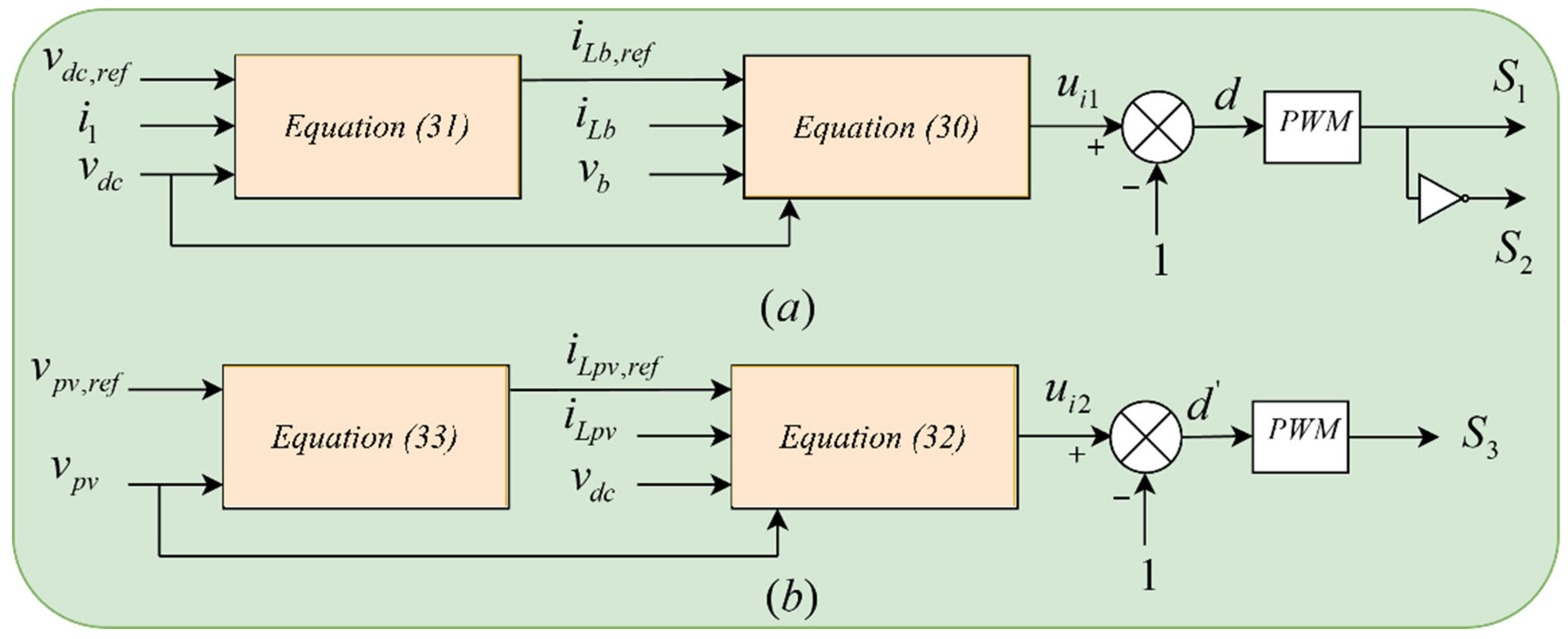
3.3. Application to DC–DC Power Converters

Since each converter is modeled using two dynamic equations, cascaded control loops are adopted. In the case of the BDC, the aim of the outer loop is to regulate the DC bus voltage and to provide a reference signal to the inner loop, which in turn takes responsibility of controlling the current flowing through the inductor $L_b$. Similarly, for the boost converter, the outer loop regulates the PV voltage while the inner loop controls the current $i_{Lpv}$.

Making use of (32), the control loops of the BDC can be described as

$$u_{i1}(t)=\frac{1}{v_{dc}}\left(\left(\frac{L_b}{T_{ri1}}+{\lambda }_{i1}\right)e_{i1}(t)+\frac{\lambda }{T_r}{\displaystyle \underset{0}{\overset{t}{\int }}{e}_{i1}(\tau )} d\tau -v_b\right)$$

(33)

$$u_{v1}(t)=-(\frac{C_{dc}}{T_{rv1}}+{\lambda }_{v1})e_{v1}(t)-\frac{\lambda }{T_r}{\displaystyle \underset{0}{\overset{t}{\int }}{e}_{v1}(\tau )} d\tau +i_1$$

(34)

The nonlinear term $\frac{P_{CPL}}{v_{dc}}$ that appears in the DC voltage dynamic equation is considered as unknown disturbance. The controller will compensate for it, which makes the system more robust against CPL power variation. Hence, the stability of the DC bus voltage will be guaranteed in large operating range.

Similarly, applying (32) to the DC–DC boost converter gives

$$u_{i2}(t)=\frac{1}{v_{dc}}\left((\frac{L_{pv}}{T_{ri2}}+{\lambda }_{i2})e_{i2}(t)+\frac{\lambda }{T_r}{\displaystyle \underset{0}{\overset{t}{\int }}{e}_{i2}(\tau )} d\tau -v_{pv}\right)$$

(35)

$$u_{v2}(t)=-(\frac{C_{dc}}{T_{rv2}}+{\lambda }_{v2})e_{v2}(t)-\frac{\lambda }{T_r}{\displaystyle \underset{0}{\overset{t}{\int }}{e}_{v2}(\tau )} d\tau +{\dot{v}}_{pv,ref}$$

(36)

The overall block diagram of the studied DC MG with its controller is depicted in Figure 3.

The proposed control structure is composed of two controllers, one for regulating the DC bus voltage and another one for regulating the PV voltage. The control diagram of the overall system is illustrated in Figure 4.

4. Simulation Results

The DC microgrid presented in Figure 2 is simulated using MATLAB/Simulink. Two controllers are designed for the PV converter and the battery converter. All the parameters of the system used in the simulations are listed in

Table 1. Simulation parameters.

Description	Parameter	Value
Parallel Resistance	$R_p$	$313.0553 \mathsf{\Omega }$
Series Resistance	$R_s$	$0.39381 \mathsf{\Omega }$
Diode Ideality Factor	$a$	$\begin{array}{c}0.98119\end{array}$
Number of Cells per Module	$N_s$	$60$
PV Open Circuit Voltage	$V_{OC}$	$160.4 \mathrm{V}$
PV Short Circuit Current	$I_{SCC}$	$8.232 \mathrm{A}$
PV Voltage at MPP	$V_{MPP}$	$128.2 \mathrm{V}$
PV Current at MPP	$I_{MPP}$	$7.718 \mathrm{A}$
PV Array Maximum Power	$P_{MPP}$	$1 \mathrm{kW}$
PV Input Capacitor	$C_{PV}$	$0.08 \mathrm{mF}$
PV Inductor	$L_{PV}$	$5 \mathrm{mH}$
DC bus Capacitor	$C_{dc}$	$1.052 \mathrm{mF}$
Nominal DC Bus Voltage	$V_{dc}$	$165 \mathrm{V}$
Nominal Battery Voltage	$V_b$	$80 \mathrm{V}$
Battery Internal Resistance	$R_i$	$0.04 \mathsf{\Omega }$
Battery Capacity	$C$	$20 \mathrm{Ah}$
Battery Inductor	$L_b$	$5 \mathrm{mH}$
Switching Frequency	$f_{sw}$	$12.5 \mathrm{kHz}$

.

By considering Equation (23) the settling time of the closed loop can be defined as $t_s\approx 4T_r$. Hence, $T_r$ should be small as possible in order to guarantee fast dynamics of the system. For switching devices, the settling time is limited by the switching frequency, and it is considered to be equal to 10 times the switching period. Thus, the predictive horizon of the inner loop for both converters is set to be equal to 0.2 ms. The outer loop should be slower than the inner loop; thus, the predictive horizon of the outer loops is set to be 2 ms. In the presence of disturbances, the closed loop error is expressed by Equation (30). It is clear that the poles associated with the transfer function are $-1/T_r$ and $-\lambda D$. The observer gain is chosen to impose the desired settling time in the presence of disturbances. The observer gain of the inner loop is set to be 0.1 for both converters. The observer gain of the outer loop of the boost converter is set to be 0.5 while the observer gain of the outer loop of the BDC is set to be 0.4.

In order to validate the proposed controller, different scenarios are performed using only pure CPL as load, which represents the worst case in terms of stability. The first scenario is performed using a CPL with small power variation and the PV power is supposed to be constant. At the beginning of the simulation, a 500 W CPL is connected to the DC bus. From 0.4 s to 0.8 s, the CPL is increased by a small step of 50 W. Starting from 0.8 s until the end of the simulation, the CPL power goes back to 500 W. As can be noticed in Figure 5, the DC bus voltage is restored at each time to its nominal value within 30 ms.

The second scenario is performed with a large CPL power variation, as depicted in Figure 6. The PV power is assumed to be constant during this scenario. Initially, a 500 W CPL is connected to DC bus. A large variation of the CPL power occurs form 0.4 s to 0.8 s, and total load power at this period is equal to 800 W. From 0.8 s to the end of the simulation, the load power steps down from 800 W to 500 W. Clearly, the controller tracks the DC bus voltage with fast dynamics and small deviation (about 2.3 V), and the DC bus voltage is restored in less than 50 ms.

Figure 7 shows the dynamics of DC bus voltage when variation occurs in the PV voltage. The PV voltage varies according to the reference given to the controller of the boost converter in the PV side. This reference is generally generated from a MPPT algorithm to achieve a maximum power under different climate conditions. The load power is maintained at 500 W during the simulation. The PV voltage takes different values that cover the operating range of the PV module. For instance, 100 V and 150 V correspond to $V_{MPP}$ at different climate conditions while 128.2 V corresponds to $V_{MPP}$ at standard test conditions. The controller is able to track the DC bus voltage reference after each variation in the PV voltage within 40 ms.

The controller is composed of two cascaded control loops with first order systems. The controller has the form of a PI controller, which is sufficient to guarantee the stability, accuracy, and robustness of the system at the same time. This is confirmed by the simulation results, i.e., the output converges to the desired setpoint for a bounded input. It is worth noting that the pole values of the closed loop system have negative real parts which ensure the system’s stability.

Another long running scenario (10 s), compared to above-mentioned ones, is performed under a square wave change of the CPL as illustrated in Figure 8. The load changes between 400 W and 600 W. Simulation results show that the common bus voltage is maintained at the desired value accordingly.

To verify the effectiveness of the proposed approach in a more realistic scenario, an integral test is performed under PV voltage fluctuation and load variation. Figure 9 shows the power flow in the studied DC microgrid. It can be seen that the PV array supplies the load and charges the battery when there is a surplus of power. Otherwise, the battery contributes to supplying the load. It can be observed from Figure 10 and Figure 11 that the PV voltage and the PV inductor current optimally track their reference values.

Similarly, Figure 12 shows that DC bus voltage tracks its reference. The stability of DC bus voltage can be seen clearly under simultaneous variation of PV power and load variation. The battery inductor current tracks the reference generated by the DC bus voltage loop, as shown in Figure 13.

It is important to emphasize that if the battery is fully charged and the PV power is greater than the load demand, an upper control layer changes the voltage reference from $V_{MPP}$ to a voltage reference. This latter corresponds to the power needed by the load. Such an operating condition is beyond the scope of this research work.

In summary, according to the above-mentioned results and considered various scenarios, we have noticed the following. In the first scenario, which was performed using a CPL while considering a small power variation and a constant PV power, the DC bus voltage is restored to its nominal value within 30 ms. Regarding the second scenario, a large power variation of the CPL is used while maintaining the PV power constant, the DC bus voltage is regulated within 50 ms. The third scenario is performed using a 500 W CPL while varying the PV power, the controller was able to maintain the DC bus voltage at the desired value. In the fourth scenario, a long simulation is conducted using a square wave change of the CPL. The controller was able to restore the DC bus voltage to its nominal value. Finally, an integral test is performed under PV voltage fluctuation and load variation. From all obtained results, the continuous-time MPC was able to stabilize the system regardless of any disturbances (e.g., CPL and PV power variations).

5. Summary and Discussion

Faced with the urgent need to reduce energy consumption and the environmental impact caused by the production of energy by traditional methods, today’s building energy production is based on various RES. This integration of diversified RESs requires the use of advanced control approaches to deal with the variable nature of the power generated by these sources. Therefore, the integration of these instable sources involves the use of energy storage systems that present the more expansive element in the whole installation with a limited lifetime. However, coupling different sources of energy with a variability of storage systems increases the complexity of the system. The deployed energy conversion components should take into consideration this complexity in order to optimize the operation of the system while achieving low consumption without sacrificing comfort. Generally, in existing systems, energy management is ensured by the installation of equipment according to the source to be integrated. Adding a source requires replacing equipment in the installed chain. For a PV installation, it is necessary to have a converter, which allows the management of energy generated by the panels. The converter makes decisions to store the energy or supply the loads. The problem with such devices is the limitation of the deployed cost functions and constraints and they are generally deployed to ensure a single objective function. The main objective of the controller is to ensure a continuous power supply to the load by extracting the maximum from the RER.

In this context, this work presents the first step towards the development of an intelligent system for power conversion. The main aim is to allow the deployment of different cost functions, such as the battery lifetime and the electricity price. The deployment of such cost functions and constraints requires the deployment of control strategies along the three control layers: primary control, secondary control, and tertiary control [19]. Mainly, the aim is to develop a converter that can deploy a predictive control approach for energy management based on the following actions: measure, analyze, predict, forecast, and execute the actions depending on the operational context. Unlike the actual converters, the main proposition considers multiple objectives functions, which take into consideration batteries’ charge/discharge cycles as well as the electricity price forecasting in order to ensure, in an optimal way, continuous electricity supply from different installed sources (e.g., RERs, batteries, utility grid) to buildings’ services. The proposed approach is based on predictive control models, which are able to generate a sequence of future control actions over a prediction horizon. However, in order to carry out this objective, several forecasted input values are required, mainly the power production/consumption and batteries’ states of charge (SoC). This requires an advanced metering infrastructure, which allows measurement and prediction of all input values. This work is a part of an ongoing research project that focuses on the deployment of a microgrid system together with an IoT/big data platform in order to conduct experiments and validate developed models.

The IoT/big data platform was developed and deployed in order to allow measurement and forecasting of RES power generation, load consumption, and batteries’ SoC. Sensing/actuating components with a control card are installed in order to monitor and manage the whole MG system, offering the possibility to test the developed control techniques in a real context. Unlike existing controllers, which are used as a black box to manage the energy in a microgrid, our future works focus on the development of an open access system to test the studied control strategies.

6. Conclusions and Perspectives

In this paper, the instability issue caused by CPLs in DC microgrids was tackled. A DC microgrid composed of a PV/battery system was considered. The dynamics of the system were described using appropriate models that take disturbances and model uncertainties into account. Based on a general model, a controller was presented using continuous-time model predictive control. Then, a disturbance observer was combined with the MPC controller in order to make it robust. The derived controller was applied for the two converters in the studied DC microgrid. Both controllers show good performances in transient response and steady state. Moreover, the controller was able to maintain the DC bus voltage at its nominal value with a fast recovery when large disturbances occur. The stability of the system is also guaranteed in a wide operating range. Simulation results show the effectiveness of the presented controller in terms of accurate tracking and stability. In our future works, more attention will be given to stability analysis of complex MG including multiple power converters and other type of loads that affects the stability, such as pulsed power loads. Regarding experiments, an open access converter is under investigations for being developed and deployed in our MG system in order to conduct experiments and assess the effectiveness of advanced control approaches.

References

1. Bazilian, M.; Onyeji, I.; Liebreich, M.; MacGill, I.; Chase, J.; Shah, J.; Gielen, D.; Arent, D.; Landfear, D.; Zhengrong, S. Re-considering the economics of photovoltaic power. Renew. Energy 2013, 53, 329–338. [Google Scholar] [CrossRef]
2. Bialasiewicz, J.T. Renewable energy systems with photovoltaic power generators: Operation and modeling. IEEE Trans. Ind. Electron. 2008, 55, 2752–2758. [Google Scholar] [CrossRef]
3. Mahmood, H.; Michaelson, D.; Jiang, J. Strategies for Independent Deployment and Autonomous Control of PV and Battery Units in Islanded Microgrids. IEEE J. Emerg. Sel. Top. Power Electron. 2015, 3, 742–755. [Google Scholar] [CrossRef]
4. NaitMalek, Y.; Najib, M.; Bakhouya, M.; Essaaidi, M. Embedded Real-time Battery State-of-Charge Forecasting in Micro-Grid Systems. Ecol. Complex. 2021, 45, 100903. [Google Scholar] [CrossRef]
5. Boulmrharj, S.; Ouladsine, R.; NaitMalek, Y.; Bakhouya, M.; Zine-dine, K.; Khaidar, M.; Siniti, M. Online battery state-of-charge estimation methods in micro-grid systems. J. Energy Storage 2020, 30, 101518. [Google Scholar] [CrossRef]
6. Boulmrharj, S.; Khaidar, M.; Bakhouya, M.; Ouladsine, R.; Siniti, M.; Zine-dine, K. Performance assessment of a hybrid system with hydrogen storage and fuel cell for cogeneration in buildings. Sustainability 2020, 12, 4832. [Google Scholar] [CrossRef]
7. Kaur, R.; Krishnasamy, V.; Kandasamy, N.K. Optimal sizing of wind–PV-based DC microgrid for telecom power supply in remote areas. IET Renew. Power Gener. 2018, 12, 859–866. [Google Scholar] [CrossRef]
8. Mahmood, H.; Michaelson, D.; Jiang, J. A power management strategy for PV/battery hybrid systems in Islanded microgrids. IEEE J. Emerg. Sel. Top. Power Electron. 2014, 2, 870–882. [Google Scholar] [CrossRef]
9. Alidrissi, Y.; Ouladsine, R.; Elmouatamid, A.; Bakhouya, M. An Energy Management Strategy for DC Microgrids with PV/Battery Systems. J. Electr. Eng. Technol. 2021, 16, 1285–1296. [Google Scholar] [CrossRef]
10. Kumar, V.; Ghosh, S.; Naidu, N.K.S.; Kamal, S.; Saket, R.K.; Nagar, S.K. Load voltage-based MPPT technique for standalone PV systems using adaptive step. Int. J. Electr. Power Energy Syst. 2021, 128, 106732. [Google Scholar] [CrossRef]
11. Kumar, N.; Hussain, I.; Singh, B.; Panigrahi, B.K. Rapid MPPT for Uniformly and Partial Shaded PV System by Using JayaDE Algorithm in Highly Fluctuating Atmospheric Conditions. IEEE Trans. Ind. Inform. 2017, 13, 2406–2416. [Google Scholar] [CrossRef]
12. Mohanty, S.; Subudhi, B.; Ray, P.K. A Grey Wolf-Assisted Perturb & Observe MPPT Algorithm for a PV System. IEEE Trans. Energy Convers. 2017, 32, 340–347. [Google Scholar] [CrossRef]
13. Emara, D.; Ezzat, M.; Abdelaziz, A.Y.; Mahmoud, K.; Lehtonen, M.; Darwish, M.M.F. Novel control strategy for enhancing microgrid operation connected to photovoltaic generation and energy storage systems. Electronics 2021, 10, 1261. [Google Scholar] [CrossRef]
14. Ali, M.N.; Mahmoud, K.; Lehtonen, M.; Darwish, M.M.F. Promising mppt methods combining metaheuristic, fuzzy-logic and ann techniques for grid-connected photovoltaic. Sensors 2021, 21, 1244. [Google Scholar] [CrossRef] [PubMed]
15. Kotra, S.; Mishra, M.K. Design and stability analysis of DC microgrid with hybrid energy storage system. IEEE Trans. Sustain. Energy 2019, 10, 1603–1612. [Google Scholar] [CrossRef]
16. Magaldi, G.L.; Serra, F.M.; de Angelo, C.H.; Montoya, O.D.; Giral-Ramírez, D.A. Voltage regulation of an isolated dc microgrid with a constant power load: A passivity-based control design. Electronics 2021, 10, 2085. [Google Scholar] [CrossRef]
17. Reddy, S.S. Optimal power flow with renewable energy resources including storage. Electr. Eng. 2017, 99, 685–695. [Google Scholar] [CrossRef]
18. Elmouatamid, A.; NaitMalek, Y.; Bakhouya, M.; Ouladsine, R.; Elkamoun, N.; Zine-Dine, K.; Khaidar, M. An energy management platform for micro-grid systems using Internet of Things and Big-data technologies. Proc. Inst. Mech. Eng. Part I J. Syst. Control Eng. 2019, 233, 904–917. [Google Scholar] [CrossRef]
19. Elmouatamid, A.; Ouladsine, R.; Bakhouya, M.; El Kamoun, N.; Khaidar, M.; Zine-Dine, K. Review of control and energy management approaches in micro-grid systems. Energies 2021, 14, 168. [Google Scholar] [CrossRef]
20. Elmouatamid, A.; Ouladsine, R.; Bakhouya, M.; El Kamoun, N.; Zine-Dine, K. A predictive control strategy for energy management in micro-grid systems. Electronics 2021, 10, 1666. [Google Scholar] [CrossRef]
21. Agarwal, A.; Deekshitha, K.; Singh, S.; Fulwani, D. Sliding mode control of a bidirectional DC/DC converter with constant power load. In Proceedings of the 2015 IEEE 1st International Conference on DC Microgrids (ICDCM), Atlanta, GA, USA, 7–10 June 2015; pp. 287–292. [Google Scholar] [CrossRef]
22. Xu, Q.; Vafamand, N.; Chen, L.; Dragicevic, T.; Xie, L.; Blaabjerg, F. Review on Advanced Control Technologies for Bidirectional DC/DC Converters in DC Microgrids. IEEE J. Emerg. Sel. Top. Power Electron. 2021, 9, 1205–1221. [Google Scholar] [CrossRef]
23. AL-Nussairi, M.K.; Bayindir, R.; Padmanaban, S.; Mihet-Popa, L.; Siano, P. Constant power loads (CPL) with Microgrids: Problem definition, stability analysis and compensation techniques. Energies 2017, 10, 1656. [Google Scholar] [CrossRef]
24. Sun, J.; Lin, W.; Hong, M.; Loparo, K.A. Voltage Regulation of DC-Microgrid with PV and Battery. IEEE Trans. Smart Grid 2020, 11, 4662–4675. [Google Scholar] [CrossRef]
25. Cespedes, M.; Xing, L.; Sun, J. Constant-power load system stabilization by passive damping. IEEE Trans. Power Electron. 2011, 26, 1832–1836. [Google Scholar] [CrossRef]
26. Ashourloo, M.; Khorsandi, A.; Mokhtari, H. Stabilization of DC microgrids with constant-power loads by an active damping method. In Proceedings of the PEDSTC 2013—4th Annual International Power Electronics, Drive Systems and Technologies Conference, Tehran, Iran, 13–14 February 2013; pp. 471–475. [Google Scholar] [CrossRef]
27. Pakdeeto, J.; Areerak, K.; Bozhko, S.; Areerak, K. Stabilization of DC MicroGrid Systems Using the Loop-Cancellation Technique. IEEE J. Emerg. Sel. Top. Power Electron. 2021, 9, 2652–2663. [Google Scholar] [CrossRef]
28. Singh, S.; Kumar, V.; Fulwani, D. Mitigation of destabilising effect of CPLs in island DC micro-grid using non-linear control. IET Power Electron. 2017, 10, 387–397. [Google Scholar] [CrossRef]
29. Xu, Q.; Zhang, C.; Wen, C.; Wang, P. A Novel Composite Nonlinear Controller for Stabilization of Constant Power Load in DC Microgrid. IEEE Trans. Smart Grid 2017, 10, 752–761. [Google Scholar] [CrossRef]
30. Xu, Q.; Blaabjerg, F.; Zhang, C.; Yang, J.; Li, S.; Xiao, J. An Offset-free Model Predictive Controller for DC/DC Boost Converter Feeding Constant Power Loads in DC Microgrids. In Proceedings of the IECON 2019—45th Annual Conference of the IEEE Industrial Electronics Society, Lisbon, Portugal, 14–17 October 2019; pp. 4045–4049. [Google Scholar] [CrossRef]
31. Vafamand, N.; Yousefizadeh, S.; Khooban, M.H.; Bendtsen, J.D.; Dragičević, T. Adaptive TS Fuzzy-Based MPC for DC Microgrids with Dynamic CPLs: Nonlinear Power Observer Approach. IEEE Syst. J. 2019, 13, 3203–3210. [Google Scholar] [CrossRef] [Green Version]
32. Andres-Martinez, O.; Flores-Tlacuahuac, A.; Ruiz-Martinez, O.F.; Mayo-Maldonado, J.C. Nonlinear Model Predictive Stabilization of DC-DC Boost Converters with Constant Power Loads. IEEE J. Emerg. Sel. Top. Power Electron. 2021, 9, 822–830. [Google Scholar] [CrossRef]
33. Errouissi, R.; Al-Durra, A.; Muyeen, S.M. A Robust Continuous-Time MPC of a DC-DC Boost Converter Interfaced with a Grid-Connected Photovoltaic System. IEEE J. Photovolt. 2016, 6, 1619–1629. [Google Scholar] [CrossRef] [Green Version]
34. Kwasinski, A. Stability analysis and stabilization of DC microgrids. In DC Distribution Systems and Microgrids; Institution of Engineering and Technology: London, UK, 2016; pp. 43–61. [Google Scholar]
35. El Mouatamid, A.; Ouladsine, R.; Bakhouya, M.; Felix, V.; Elkamoun, N.; Zine-Dine, K.; Khaidar, M.; Abid, R. Modeling and Performance Evaluation of Photovoltaic Systems. In Proceedings of the 2017 International Renewable and Sustainable Energy Conference IRSEC 2017, Tangier, Morocco, 4–7 December 2017; pp. 1–7. [Google Scholar] [CrossRef]
36. Tremblay, O.; Dessaint, L.A. Experimental validation of a battery dynamic model for EV applications. In Proceedings of the 24th International Battery, Hybrid and Fuel Cell Electric Vehicle Symposium & Exhibition 2009: (EVS 24), Stavanger, Norway, 13–16 May 2009; Volume 2, pp. 930–939. [Google Scholar]
37. Yang, J.; Zheng, W.X. Offset-free nonlinear MPC for mismatched disturbance attenuation with application to a static var compensator. IEEE Trans. Circuits Syst. II Express Briefs 2014, 61, 49–53. [Google Scholar] [CrossRef]
38. Yang, J.; Zheng, W.X.; Li, S.; Wu, B.; Cheng, M. Design of a prediction-accuracy-enhanced continuous-time MPC for disturbed systems via a disturbance observer. IEEE Trans. Ind. Electron. 2015, 62, 5807–5816. [Google Scholar] [CrossRef]
39. Xu, Q.; Yan, Y.; Zhang, C.; Dragicevic, T.; Blaabjerg, F. An Offset-Free Composite Model Predictive Control Strategy for DC/DC Buck Converter Feeding Constant Power Loads. IEEE Trans. Power Electron. 2020, 35, 5331–5342. [Google Scholar] [CrossRef]
40. Wallscheid, O.; Ngoumtsa, E.F.B. Investigation of Disturbance Observers for Model Predictive Current Control in Electric Drives. IEEE Trans. Power Electron. 2020, 35, 13563–13572. [Google Scholar] [CrossRef]
41. He, W.; Li, S.; Yang, J.; Wang, Z. Incremental passivity based control for DC-DC boost converter with circuit parameter perturbations using nonlinear disturbance observer. In Proceedings of the IECON 2016—42nd Annual Conference of the IEEE Industrial Electronics Society, Florence, Italy, 24–27 October 2016; pp. 1353–1358. [Google Scholar] [CrossRef]
Figure 1. A typical DC microgrid with CPLs.
Electronics 11 01481 g001
Figure 2. The studied DC microgrid.
Electronics 11 01481 g002
Figure 3. Overall block diagram of the system.
Electronics 11 01481 g003
Figure 4. Control schemes for (a) DC–DC bidirectional converter (b) DC–DC boost converter.
Electronics 11 01481 g004
Figure 5. Simulation results with small CPL power variation.
Electronics 11 01481 g005
Figure 6. Simulation results with large CPL power variation.
Electronics 11 01481 g006
Figure 7. Simulation results under PV voltage variation and fixed CPL.
Electronics 11 01481 g007
Figure 8. Simulation results under a square wave change of the CPL.
Electronics 11 01481 g008
Figure 9. PV power, battery power, and load power.
Electronics 11 01481 g009
Figure 10. PV voltage.
Electronics 11 01481 g010
Figure 11. PV inductor current.
Electronics 11 01481 g011
Figure 12. DC bus voltage.
Electronics 11 01481 g012
Figure 13. Battery inductor current.
Electronics 11 01481 g013