EMI Minimization from Stacked Radiation Sources by Means of Multiple Objective Genetic Algorithm

Abstract

The containment of unwanted electromagnetic radiation and interference is a relevant topic for the system design of any electrical system, and even more for data centers. In this context, the racks hosting piles of servers are one of the main sources of electromagnetic noise. Such unwanted radiation can couple and interact with other computing machines, but also with sensitive electronic devices needed for the management and/or maintenance of the center. The aim of this work is to show how the proper stack-up of the trays in the rack gives rise to a decrease in the unwanted physical electromagnetic radiation. Based on the application of the spherical wave expansion technique, a multi-objective genetic algorithm is developed to evaluate the optimal set of rack configurations that allows for a reduction of the external radiated field. The algorithm and the implemented constraints are described, and the results are discussed.

1. Introduction

The ever-growing demand for computing power, storage services, and communication bandwidth brings evident challenges to the design of data centers and their constitutive parts. The server’s racks are made up of several trays, vertically stacked. They absorb electric power, part of which is dissipated in the form of heat, and need to be cooled. Among the design strategies for passive cooling, there is the tendency of reducing any unnecessary heat barriers, such as parts of the tray enclosure. This design trend shows some drawbacks from the electromagnetic compatibility point of view. In fact, the lack of parts of the metallic enclosure decreases the overall electromagnetic shielding of each tray, increasing its unwanted radiation toward the other trays of the same rack and toward the space external to the rack.

In modern data centers, in the aisles in between the racks, electronic devices such as personal computers or tablets of the maintenance personnel, or other electronic circuits used for different operations, are often present. Both classes of device are very sensitive to electromagnetic interference (EMI), and can be affected by the unwanted electromagnetic field radiated by the trays in the racks.

One more aspect to be considered is the high connectivity of the data center environment. Multiple wireless systems supervise the normal and maintenance operations of the center. The above-mentioned decreased shielding performance of the trays allow the trays’ electromagnetic fields to interact with the communication signals which, in turn, can be a source of interference for the trays’ electronic circuits.

In [1], an efficient approach has been developed based on spherical wave expansion (SWE) theory [2] to evaluate the total unwanted electromagnetic radiation of multiple stacked trays, considered as radiation sources, starting from the knowledge of the radiation characteristic of each single source considered isolated. The methodology in [1] has been applied, in [3], to the measured radiation pattern of a real rack. Each tray forming the rack has been characterized by the SWE coefficients, which are extracted by the direct measurements of its radiation fields when considered in isolation. These measurements consider each tray’s functionality and setting. From [3], a sort of library of SWE coefficients for each tray typology is made available to reconstruct the total electromagnetic field, due to the stacking of the trays and for further elaboration.

The target of this paper is to develop a procedure to find the optimal position of the trays in the vertical stack of a rack, in order to minimize their total physical electromagnetic radiation in a volume of space outside the rack. This procedure, formally set as a minimization problem, will resort to the SWE coefficients of the trays for the efficient computation of their radiation, and to a multi-objective optimization approach based on a genetic algorithm (MOGA) [4].

Section 2 illustrates the physical model of the trays and racks, briefly recalls the extraction and use of the associated SWE coefficients, and describes the target volume of space for which the cost functions are defined. The implemented MOGA and some constraints set on the formation of the chromosomes, in order to take into account the actual design of a rack (aka rackification), are introduced in Section 3. The results, all in terms of electromagnetic fields, their comparison with those obtained by other methods, and the practical implications of multiple solutions that are not optimal, with respect to all objectives, are discussed in Section 4. Finally, Section 5 offers some concluding remarks.

2. The Radiation Source: Model and Target Volume

2.1. Model of the Radiation Source

The source of radiation considered in this work is a servers’ rack. This functional structure is built by the piling-up of several active units, called trays, that perform the different operations of a data center: computing, storage, networking, etc. Figure 1 shows a schematic representation of the rack structure considered in this work, featuring a total of nine trays of three different typologies, named, for sake of generality, Bot, Mid, and Top.

In [1], it has been shown that the use of the SWE technique is an efficient way to evaluate the electromagnetic field radiated from a single tray by reconstructing the tray radiation from the SWE coefficients. Among the advantages, this technique considers the total field embodying the local reflections and, in analogy with traditional numerical techniques such as the method of moments, the SWE technique does not need any boundary condition. Additionally, in [1], a mathematical procedure to assemble such coefficients to compute the total radiation of more than one tray has been developed, applied, and validated. Hence, the critical point is the availability of the SWE coefficients. In [3,4], a library of SWE coefficients is obtained for the different typologies (Top, Mid, and Bot) of operating trays from accurate radiation measurements, performed in an anechoic chamber, and by the application of a genetic algorithm (GA) optimization. In this way, the SWE coefficients contain all the relevant information of the functioning tray, from which the input and output power, bandwidth, and relevant harmonics are extracted, which will also appear in the reconstructed field with a given approximation [3].

Based on these conceptual blocks, the radiation source of this work is the stack of trays in Figure 1. In general, rack-mountable equipment is traditionally mounted by bolting or clipping its front panel to the rack. Within the network industry, it is common for server trays to have multiple mounting positions, so rack-mountable equipment will often feature L-brackets that must be screwed or bolted to the equipment prior to mounting on a 45 cm rack. Servers and deep-set pieces of equipment are often mounted using rails that are bolted to the front and rear posts, allowing the equipment to be supported while also enabling it to be easily installed and removed. Although there is no standard for the depth of equipment, there is a tendency for four-or-more-post racks to be between 60 cm and 100 cm deep: in our case, the rack depth is 60 cm. The materials of the structural parts of the racks and trays are usually made of steel of around 2 mm thickness, or of slightly thicker aluminum.

The geometry of the rack has been simplified (because not all the mechanical and structural information can be disclosed), but maintains the relevant features for the target of this work. The total height of the rack is h_r = 174 cm, its width is w_r = 45 cm, and its frontal length is l_r = 60 cm. Each try has w_t = w_r, l_t = l_r, and h_t = 8 cm. The lowest tray in the stack is placed h_t0 = 100 cm from the ground.

For each combination of the trays’ position in the stack, the electromagnetic field is computed, and as described in Section 3, its minimum is sought in the specific volume described in the next sub-section.

2.2. The Target Volume for EMI Minimization

The target volume in which the minimization of the electromagnetic field should be enforced, due to the combination of the radiation of the trays in the rack, is located in front of the rack, where the presence of susceptible electronic devices can be assumed. Figure 2 helps to visualize the position and the form of the volume. In modern data centers, two kind of devices with electronic circuits that are susceptible to electromagnetic interferences are present in front of the racks:

• Those that are usually located in the lower part of the volume (named Volume 1 or V₁, in yellow in Figure 2), up to h_V1 = 60 cm from the ground, spanning the full width of the aisle (w_V1 = 200 cm);
• Personal information devices, such as personal computers, tablets, and smartphones. They are associated with the personnel and are usually located in the upper part of the volume (named Volume 2 or V₂, in green in Figure 2), from h_V1 to h_V2 = 170 cm. The width of V₂ is narrower than that of V₁: w_V2 = 150 cm.

In each volume, a number, N₁ and N₂, of test points are defined and used to compute two independent cost functions, f_c1 and f_c2—one for each volume.

The generic cost function f_ci (for i = 1,2) is defined as:

$$f_{ci}={\left|E_{avgi}-E_{thi}\right|}_{,}$$

(1)

where:

• E_avgi is the average value of the electric field, computed on N_i test points in volume V_i;
• E_thi is the threshold value of the electric field, above which the EMI matters. This value could be obtained by the standards and/or by specific design rules. In this work, without loss of generality, the threshold values, stemming from particular applications, are E_th1 = 1 μV/m and E_th2 = 1.5 μV/m, respectively.

In the following, N₁ = 8 will be considered in volume V₁, and N₂ = 8 equally spaced test points will be considered for volume V₂.

3. Constrained Multiple Objective Genetic Algorithm

Genetic algorithms (GA) follow a heuristic procedure to solve the research problems of the optimal solution(s). They consider a set of solutions (called chromosomes or individuals) that evolve in intervals of time called generations. Evolution is driven by the comparison of the values of cost (or objective or fitness) functions [5], evaluated for each chromosome of the population. These functions are a sort of measure of quality, with respect to the problem considered. By means of these values, individuals of one generation are compared, selected, and used to create the population of the next one, which is formed by individuals with better cost function values. 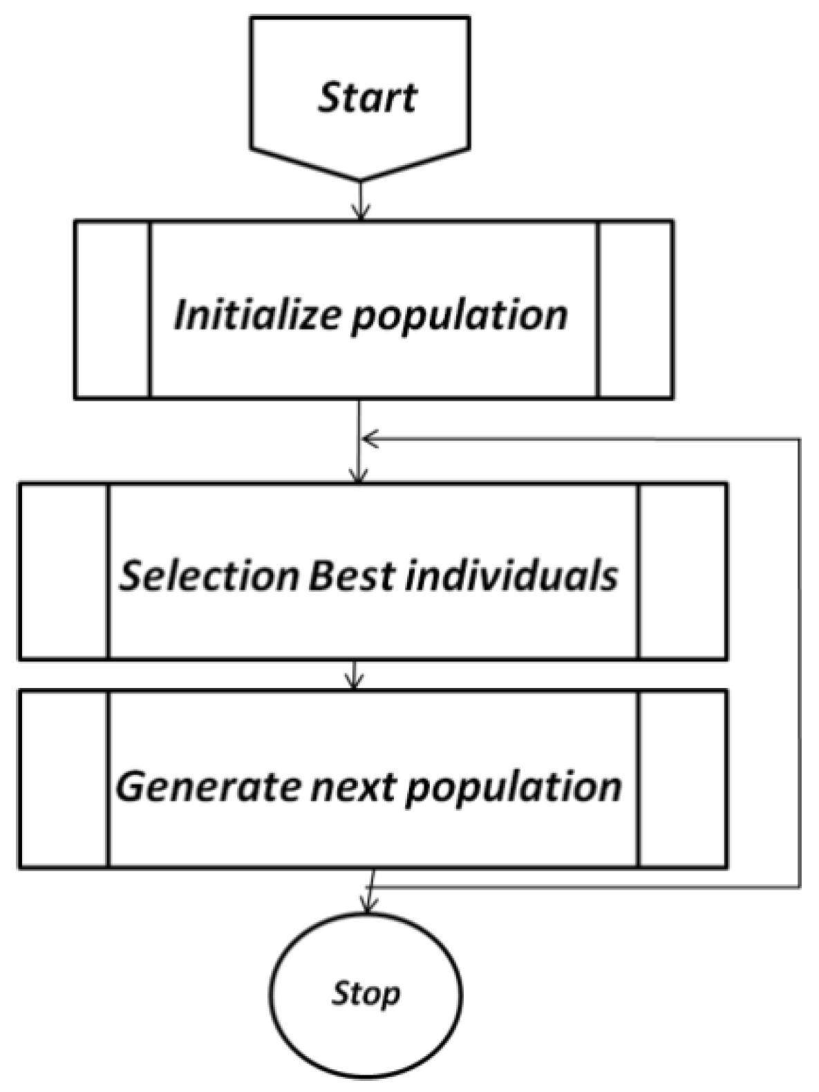The basic structure of a genetic algorithm is cyclic and is shown in Figure 3. Each cycle represents a generation, and within it, operations are carried out to generate a newly formed population with increasingly better chromosomes.

The first step of the algorithm is to create a random population of chromosomes. The following phases are repeated with each generation, and are associated with the principle of natural selection: the early stages are concerned with selecting the best individuals in the population, while the others generate new individuals.

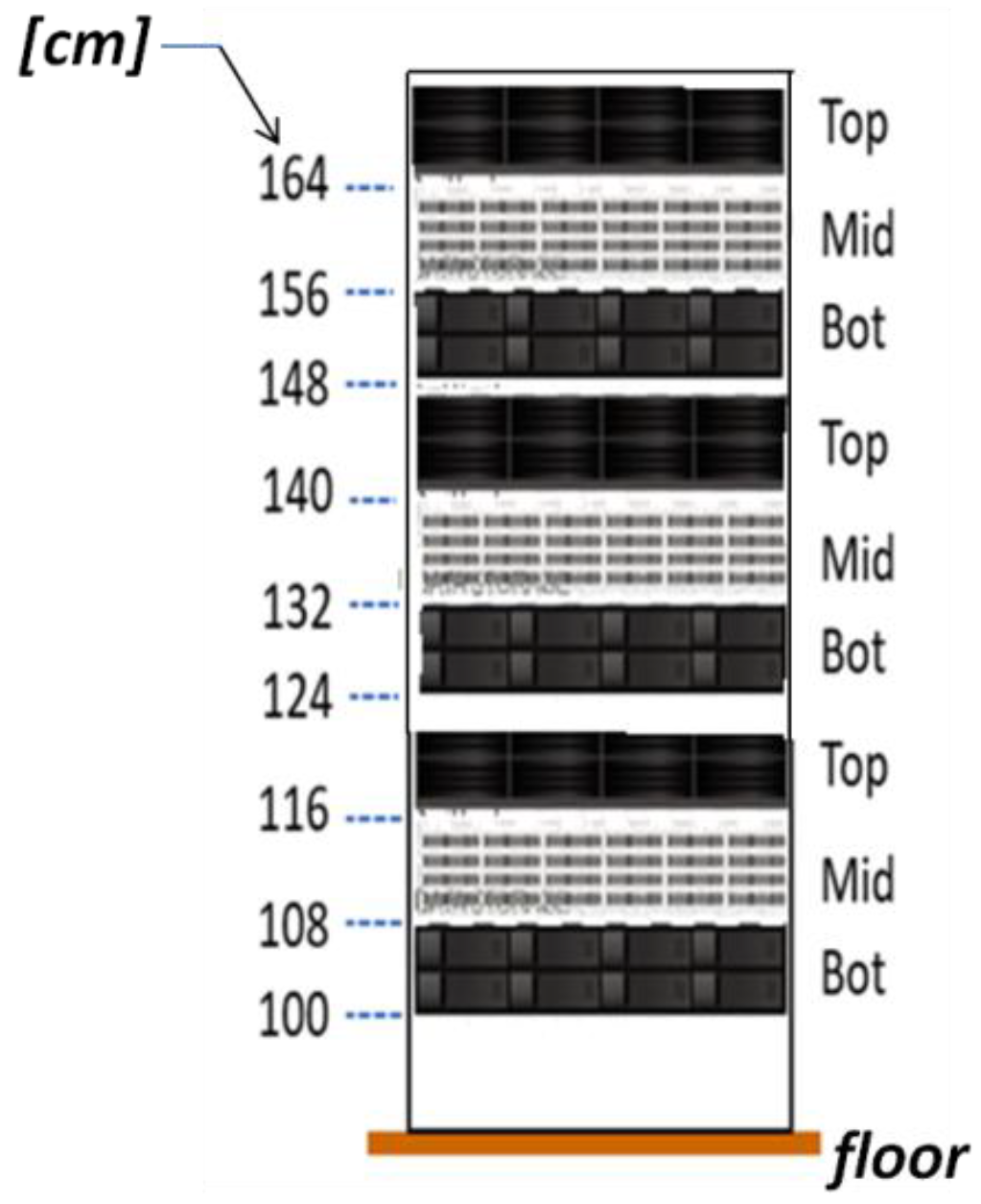
Chromosomes are the basis of the functioning of the genetic algorithm, and they represent possible solutions to the problem. In our case, each chromosome is built up by N_g = nine genes. Each gene represents one of the nine trays of the rack, as in Figure 1. The first gene is associated with the bottom-most tray at h_t0 = 100 cm, the second gene with the tray at h_t = 108 cm, and so on. The value of a gene can have only three integer values (1, 2, or 3), which are associated with the proper set of SWE coefficients of the Bot, Mid, and Top trays, respectively. The number of chromosomes in the population is N_c = 500.

At this stage of the algorithm, new chromosomes are generated from other chromosomes bypassing their own genetic heritage, so that the new solutions are similar but not equal to the parent ones. This aspect is fundamental for the convergence of the algorithm; in fact, every new population is built with better individuals than the previous one. This is the crossover phase. In this work, the whole arithmetic crossover has been used [6], where the new chromosomes (or offsprings) are a linear combination of the two parent chromosomes. In this technique, a pair of chromosomes are selected randomly for crossover, and by a linear combination, two new ones are produced. This linear combination can be described as:

$$offspring1=\alpha \ast Parents{1}_1+\left(1-\alpha \right)\ast Parents{2}_2,$$

(2)

$$offspring2=\alpha \ast Parents{1}_2+\left(1-\alpha \right)\ast Parents{2}_1,$$

(3)

where offspringi is the i-th offspring (i = 1, 2), Parentsi_j is the j-th part (j = 1 corresponds to the first m genes of the i-th chromosome Parentsi, j = 2 corresponds to the remaining 9-m genes of the i-th chromosome Parentsi), and m is a random number, such that 2 < m < 8.

The next step is the application of the mutation operator. The effect of this operator is to deeply modify the chromosome so that the mutated individual explores areas of the space of solutions not yet observed. This phase is introduced to avoid convergence towards local optimal minima or maxima, thus favoring a global search. In this work, a mutation rate of μ = 20% has been used, which corresponds to about 900 gene mutations. Random numbers, chosen from a Gaussian distribution, are chosen to select the gene to mutate, and its value is replaced by another random value between 1 and 3.

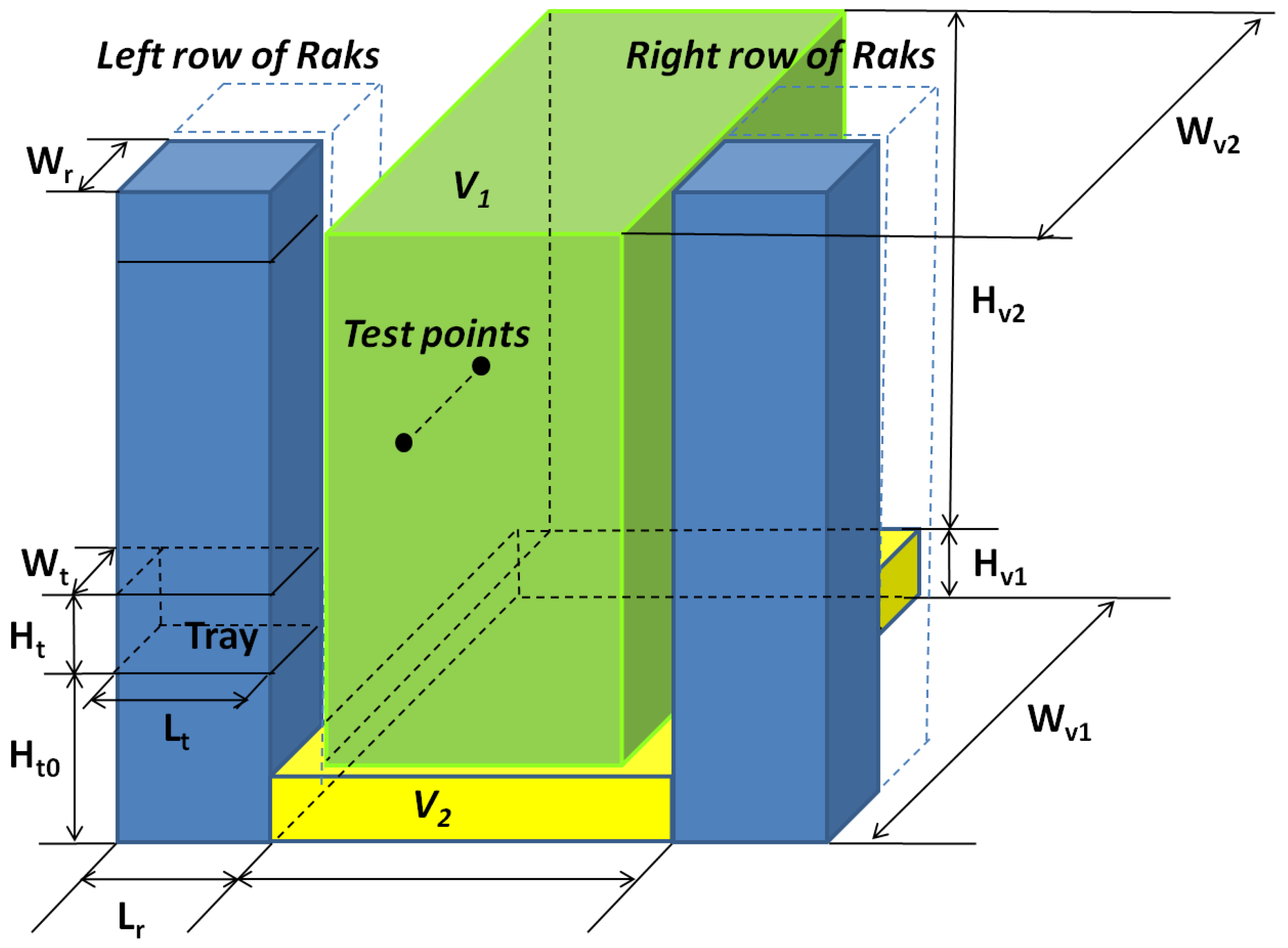
The part of the algorithm inspired by the principle of natural selection deals with the classification of chromosomes, and ranks and selects the best solutions within the population. The cost functions f_c1 and f_c2 for volumes V₁ and V₂, as defined in Equation (1), are used as measures of the fitness of the solutions. Different from a single-objective GA, in a multi-objective approach, the two cost functions are not combined into one [3,7], but are considered separate.

Once the fitness of each chromosome is calculated, a subpopulation is chosen to generate new solutions. There are various techniques for selecting the set of solutions, named the mating pool, for reproduction. Due to the large number of the population used in this work (the size is N_p = 500 chromosomes), the tournament selection technique has been chosen [8]: a small subset of chromosomes (in this work, the size of this subset is 4) is randomly picked up from the mating pool, and the chromosomes with the lowest f_ci in the subset become parents. The tournament repeats for every offspring needed. In the tournament selection, the whole population never needs to be sorted; this is a clear advantage because it is known that sorting is a time-consuming action for large populations.

The multi-objective nature of the developed algorithm is shown by evaluating the f_c1 for volume 1 and the f_c2 for volume 2 (f_ci is defined in Equation (1)) separately for each chromosome of the population, instead of merging them in a single weighted cost function [9]. At each chromosome, both values of f_ci are associated, forming a point of coordinates (f_c1, f_c2) in the cost function Cartesian plane. At each chromosome (at each point on the plane), the concept of dominance is applied, and only the non-dominated chromosomes belonging to the Pareto front [10] are retained as optimal solutions. 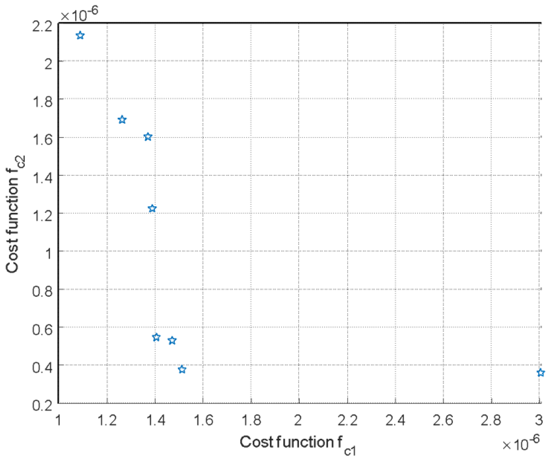Figure 4 qualitatively shows six solutions, of which only four are non-dominated, forming the optimal solutions’ Pareto fronts. Without adding additional information, all four solutions are equally satisfactory. This flexibility is one of the strengths of the MOGA.

In order to make the MOGA implementation more suitable for its use in the design of the stack of trays from the point of view of the unwanted radiation, the presence of a specific design constraint is considered. In the real design of a rack, there is a limit on the repetition of the same tray in the stack. A rack cannot be formed by trays of the same type. This constraint is introduced in the algorithm in the form of a soft constrained technique [11,12] that is considered more valid for real and complex problems than a hard one. The soft constrained technique implemented is the penalty function method. This method penalizes the cost functions of solutions that are not eligible. In this way, chromosomes are moved to areas of the space of the goals that the ranking considers worse. This is completed in two simple steps: first, whether the chromosomes respect the constraint (i.e., the number of genes with the same value is less than a given constrain value K) is checked. Subsequently, the values of the cost functions associated with these individuals are increased by a factor R_c that moves their chromosomes far from the optimal region, and then excludes them from participating in the new generations. In the next section, a systematic analysis of the impact of the constraint value K on the optimal solutions will be carried out.

4. Results and Discussion

As the first step for a critical discussion of the numerical output, a set of reference results needs to be compared with those stemming from the proposed MOGA. These reference results are found by using the analytical procedures developed in [3,4], where a single-objective GA (SOGA) has been developed. The implemented SOGA finds the minimum unwanted radiated EMI in volumes V₁ and V₂ at a specific frequency that is considered critical for the applications considered. As mentioned, the results obtained by the SOGA are considered as a sort of reference for those stemming from the MOGA, either to show the similarities or to show the differences, advantages, and drawbacks. For the SOGA, the two cost functions f_c1 and f_c2 (defined in Equation (1)) are combined into the single f_cSOGA:

$$f_{c\mathrm{SOGA}}=f_{c1}+f_{c2}=\left|E_{avg1}-E_{th1}\right|+\left|E_{avg2}-E_{th2}\right|,$$

(4)

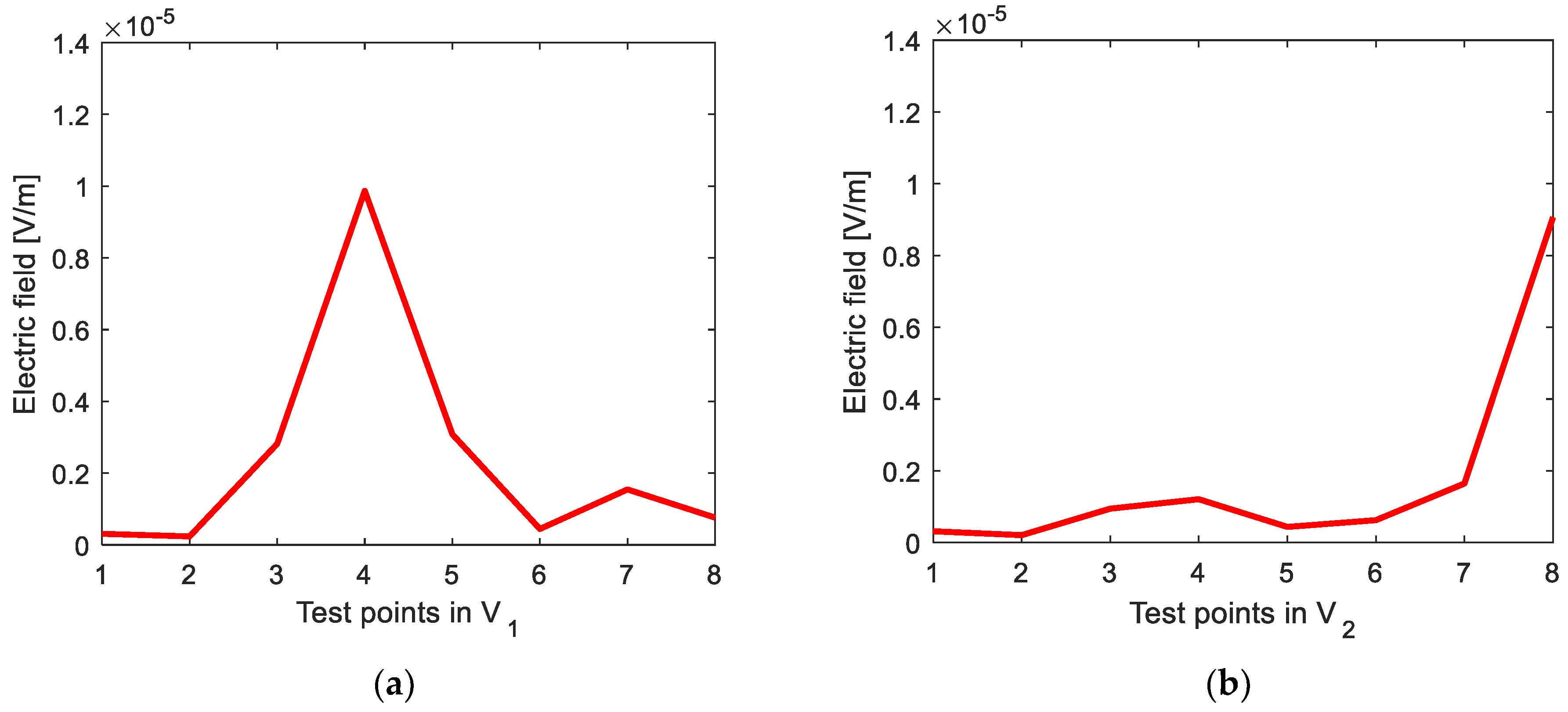
ensuring similar conditions between the SOGA and the MOGA. Figure 5a,b reports the magnitude of the computed radiated electric field in each of the N₁ and N₂ test points in the volumes, due to the configuration of the trays in the rack that minimizes Equation (5), according to the SOGA. Such optimal configuration is represented by the chromosome C_SOGA:

C_SOGA = [ 3 1 3 2 2 2 2 2 2 ],

(5)

in which:

• The first element of the chromosome corresponds to the bottom-most tray in Figure 1;
• The tray typology coding is 1 = Bot, 2 = Mid, and 3 = Top.

Figure 5. The magnitude of the electric field in (a) the N₁ test points of volume V₁ and (b) the N₂ test points of volume V₂, due to the optimal SOGA solution C_SOGA in Equation (6).

Figure 5. The magnitude of the electric field in (a) the N₁ test points of volume V₁ and (b) the N₂ test points of volume V₂, due to the optimal SOGA solution C_SOGA in Equation (6).

The structure of the SOGA chromosome is the same as the structure of the MOGA one. The results in Figure 5 are considered as the reference results for all the subsequent structures.

The second step considers the MOGA’s optimal solutions. As mentioned in Section 3, the output of a MOGA procedure is a set of solutions (in our case, a set of tray configurations), each one non-dominated by the others: they form the optimal Pareto front. The optimal Pareto front obtained for the problem at hand, characterized by the same variables of the SOGA, is given in Figure 6.

In Figure 6, each starlet indicates a chromosome, or a tray configuration. The eight chromosomes, from C_MOGA1 to C_MOGA8, of the optimal Pareto front in Figure 6 are reported, by row, in

Table 1. Chromosomes belonging to the optimal Pareto front in Figure 6. The tray typology coding is: 1 = Bot, 2 = Mid, and 3 = Top.

Gene	g1	g2	g3	g4	g5	g6	g7	g8	g9
CMOGA1	2	2	2	2	2	2	2	2	2
CMOGA2	2	2	2	2	2	2	2	3	3
CMOGA3	2	2	3	3	2	2	2	2	2
CMOGA4	3	2	2	2	2	2	2	2	2
CMOGA5	3	3	2	2	3	3	2	2	2
CMOGA6	3	3	2	3	2	3	3	3	2
CMOGA7	3	3	3	2	2	3	3	2	2
CMOGA8	3	3	3	3	3	3	3	3	2

.

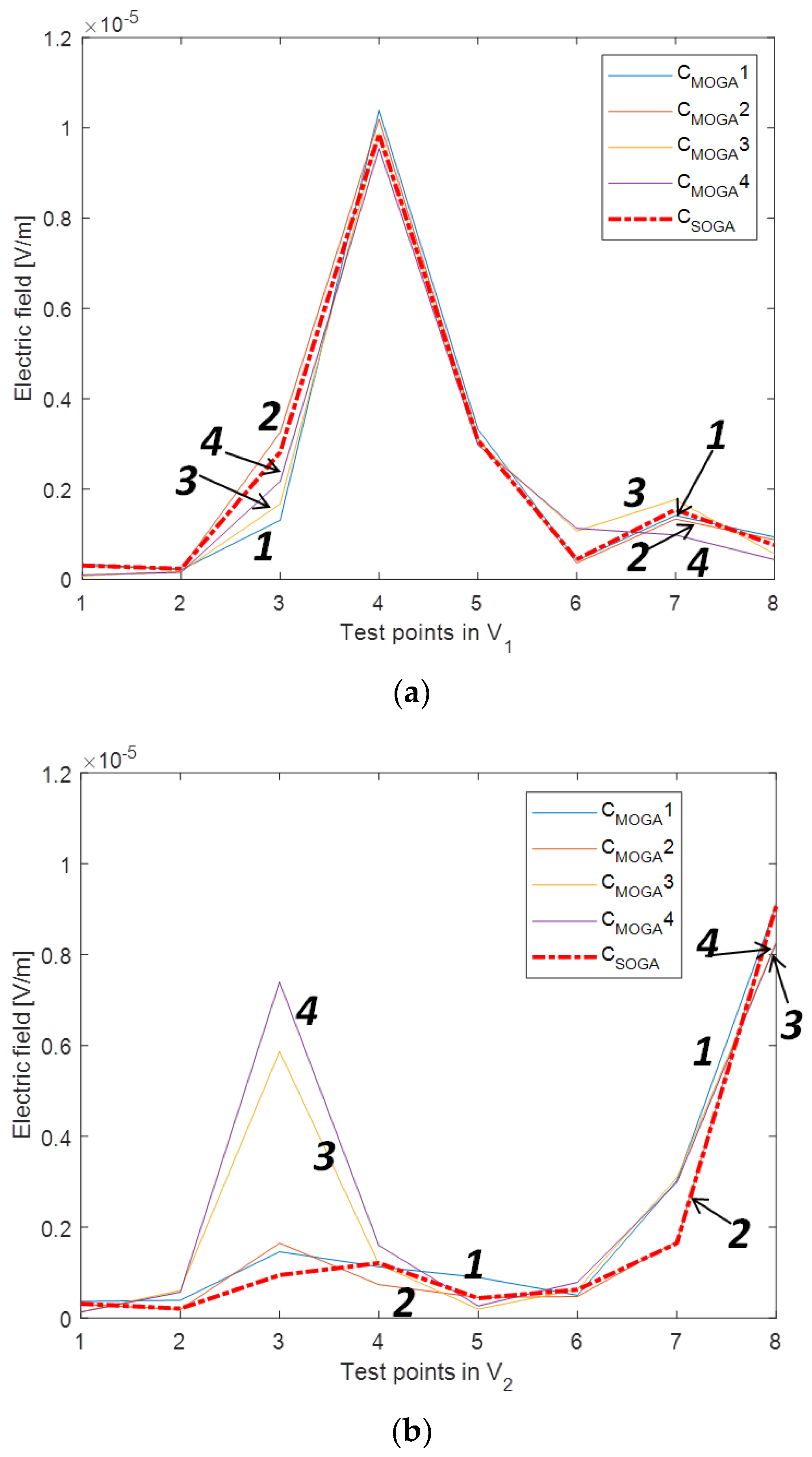
At each of the rack’s configurations, described in Table 1, and belonging to the optimal Pareto front, corresponds a value of the magnitude of the computed electromagnetic radiated field in the N₁ and N₂ points of volumes V₁ and V₂, respectively. Figure 7a,b shows these magnitudes in these test points radiated by the configurations of the trays in Table 1 that minimize Equation (5), according to the proposed MOGA. They are also compared, as reference, with the field distribution in the same test points, due to the chromosome C_SOGA in Equation (6).

In general, as expected, the spatial distribution of the radiated field estimated by the SOGA and MOGA algorithms are similar but not identical. The values of the electric field, due to the configurations C_MOGA1, C_MOGA4, and C_MOGA8 (those with the starlets close to the origin of the axis in Figure 6), are closer to C_SOGA. The others have higher magnitudes, but still belong to the optimal Pareto front and are an option if other design limitations or constraints must be taken into account.

In the design process of a server rack, there is a great number of logical and physical constraints to consider when positioning the trays. In the logical class fall those related to the functionality and principal operations for which the rack is targeted (processing, storage, switching, etc.); to the physical class belongs those limits such as overall weight, length of the interconnection cables/fibers, and total heat dissipated. For this reason, as the third step of the analysis of the results, a procedure to limit the number of repetitions N_r of trays of the same type in the rack has been added to the proposed MOGA without constraints. This constraint is an indirect but efficient way to consider either the logical or functional design limits [11,12]. The value N_r ranges from N_g (a rack of all equal trays) to N_r = 3, which is the minimum number of tray repetitions given the three different types of trays (Top, Mid, and Bot). Based on this, the impact of several values of the constraint N_r is considered, and is shown in the following figures and tables.

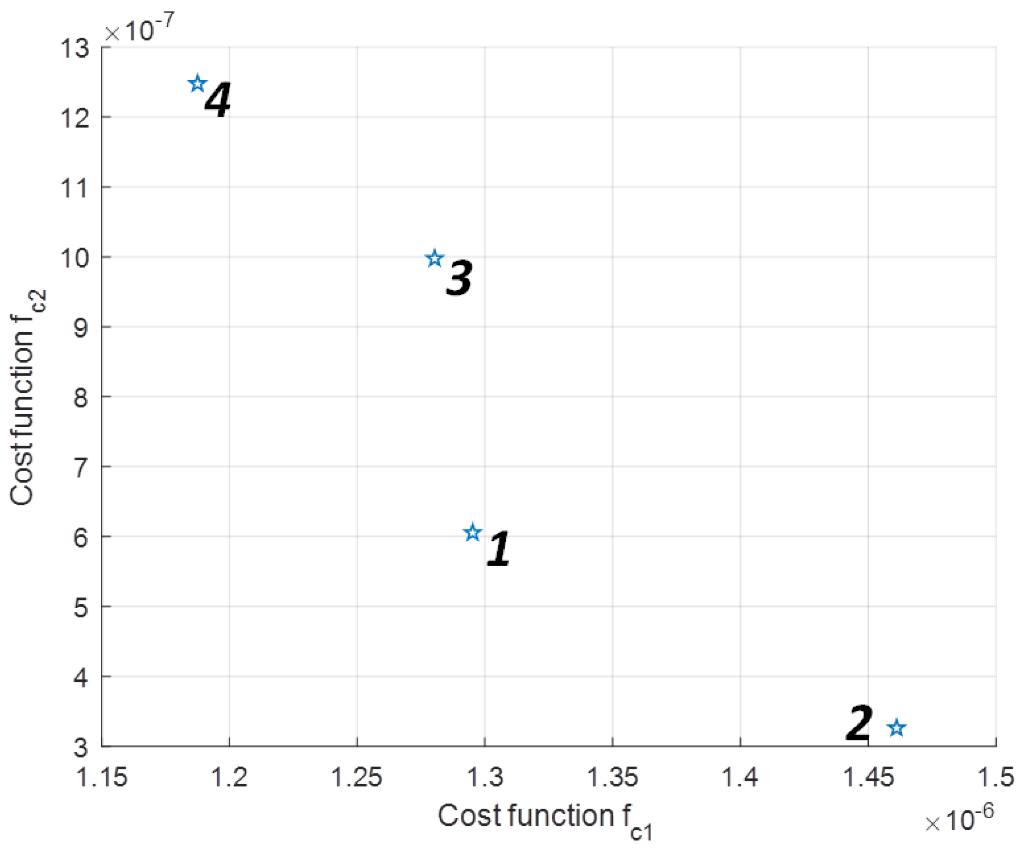
Setting N_r = 5 yields the optimal solutions obtained by the proposed constrained MOGA, shown in Figure 8 (obtained by [13]), to which the chromosomes in

Table 2. Chromosomes belonging to the optimal Pareto front in Figure 8, considering the constraints N_r = 5. The tray typology coding is 1 = Bot, 2 = Mid, and 3 = Top.

Gene	g1	g2	g3	g4	g5	g6	g7	g8	g9
CMOGA1	2	2	1	3	2	1	3	2	2
CMOGA2	3	1	3	1	3	2	2	2	2
CMOGA3	3	3	2	2	1	3	2	1	1
CMOGA4	3	3	2	2	2	2	2	1	1

correspond.

The spatial distributions of the magnitude of the electric field in the N₁ and N₂ test points in volumes V₁ and V₂, due to the four optimal configurations in Figure 8 and obtained by imposing the constrain N_r = 5, are shown in Figure 9, along with, as reference, the values of the electric field in the same points obtained by the configuration in C_SOGA in Equation (6).

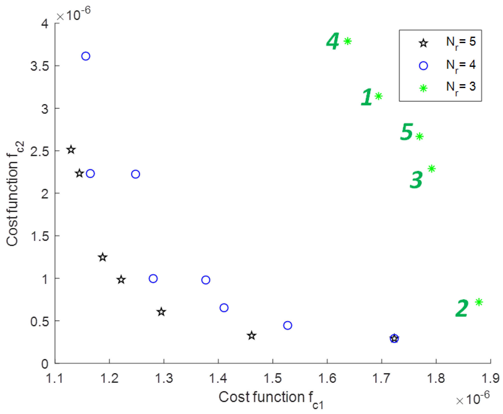
As the N_r decreases (from 9 to 3), the constraint becomes stricter, the number of possible tray repetitions decreases and, hence, the performance of the optimal solutions that show an increase in the values of the cost functions also decreases. This is visible in Figure 10, where the optimal solutions for N_r = 5, 4, and 3 move from the region close to the origin of the axis to regions with larger values of f_c1 and f_c2, respectively.

Table 3. Chromosomes belonging to the optimal Pareto front in Figure 10, considering the constraints N_r = 3. The tray typology coding is 1 = Bot, 2 = Mid, and 3 = Top.

Gene	g1	g2	g3	g4	g5	g6	g7	g8	g9
CMOGA1	1	3	1	1	2	3	3	2	2
CMOGA2	2	1	3	2	1	3	2	1	3
CMOGA3	2	3	1	2	2	1	1	3	3
CMOGA4	3	3	1	2	2	3	1	1	2

connects the solutions in Figure 10 with the disposition of the trays in the rack fulfilling the stricter constraint of N_r = 3.

The inherent statistical nature of a GA calls, at least, for the evaluation of its performance for multiple runs to test the convergence of the computed output. For the specific physical problem considered up to now, the optimal Pareto front for seven cases has been computed: the unconstrained MOGA (or N_r = 0), and the MOGA with N_r = 3, 4, 5, 6, 7, and 8. Each case has been run 100 times, and the 100 optimal Pareto fronts for each case have been plotted in Figure 11. The runs for N_r = 8 (purple circles) are very close to the unconstrained case, as expected. As the constraints become stricter (N_r decreases), the cluster of fronts moves forward from the origin of the axis toward regions of higher values of the cost functions. Please note that different runs can produce chromosomes with the same structure, so some symbols are overlapped.

From a visual inspection of Figure 11, the self-consistency of the results and the accuracy of the MOGA is evident: the less stringent the constraint, the more solutions with low cost function values are available, giving rise to a cluster of symbols close to the origin of the axis. As the constraint becomes more stringent, less configurations are available, so the optimal solutions move far from the low values of the f_ci that also spread on the f_c1–f_c2 plane. This is confirmed as a proper quantitative measure of the Cartesian distance of each solution from the origin of the axis. For the generic i-th solution, the distance d_i is defined as:

$$d_i=\sqrt{f_{c1i}^2+f_{c2i}^2}.$$

(6)

For each set of constraints, N_r, one can compute the average distance D and the standard deviation σ of all the solutions belonging to that constraint.

Table 4. Statistical properties of optimal Pareto fronts in Figure 11.

	Unconstrained	Nr = 8	Nr = 7	Nr = 6	Nr = 5	Nr = 4	Nr = 3
D	1.91 × 10−6	1.99 × 10−6	2.14 × 10−6	2.20 × 10−6	2.24 × 10−6	2.37 × 10−6	2.54 × 10−6
σ	5.48 × 10−7	5.31 × 10−7	4.86 × 10−7	5.57 × 10−7	7.38 × 10−7	7.18 × 10−7	8.42 × 10−7

reports the results. The qualitative trends are confirmed by the values in the table.

As final consideration, it is worthy to quantify the radiated field attenuation obtained by the optimal configuration of the trays in the stack of the rack. Figure 12a,b shows the spatial distribution of the magnitude of the electric field in the test points of V₁ and V₂, due to the complete population of chromosomes (100 curves).

In the entire population, the distribution due to one of the optimal MOGA solutions belonging to the Pareto front is highlighted in red. The attenuation between the overall maximum value in the population and the maximum of the optimal solution is around 6 dB for V₁ and around 4.8 for V₂.

5. Conclusions

The use of the spherical wave expansion technique as a practical and efficient means to compute the electromagnetic field radiated by complex assemblies of sources, each one experimentally characterized in terms of its SWE coefficients, has opened the possibility of optimizing the radiation performances. In this work, this technique has been applied to the minimization of the unwanted radiation in the space in front of a server rack by choosing the proper sequence for the vertical allocation of the server trays in the rack. To do this, two genetic algorithms, SOGA and MOGA, have been developed. The MOGA has shown the same accuracy as the SOGA, but has more flexibility because its set of multiple optimal solutions, instead of the single one of the SOGA, allows for choices based on other criteria. To make the proposed MOGA approach more suitable for engineering applications, a constraint strategy has also been implemented, limiting the repetitions of the same tray in the rack to a selectable number. The results are in line with the expectations. We have not yet compared the proposed results with those obtained by other algorithms because the present paper describes the second of a three-phase project. The next stage of this research project is the execution of a measurement campaign, whose results could help to refine the accuracy of the proposed optimization strategy and the electromagnetic field evaluation model.