
Resource-Efficient Hardware Implementation of Perspective Transformation Based on Central Projection


Abstract
1. Introduction
- The transformation method of the central projection has been improved, and two variable parameters have been added, so that it can achieve a similar effect to the homography transformation.
- The hardware design of perspective transformation based on the central projection transformation is proposed. Compared with the most used homography transformation, it is simpler, and the hardware does all the calculations.
- It has excellent compatibility. According to actual application scenarios, the calculation speed and required resources can be flexibly adjusted by increasing or decreasing the number of pixel calculation modules. When the degree of parallelism is one, it requires 2893 Look-up Tables (LUTs), which can process resolution video at 20 Hz, and when the degree of parallelism is eight, it is 11,223 LUTs, which can process 157 Hz video streams.
- The design of this paper is more practical; it can complete many image transformations, such as scaling, translation, tilt correction, BEV and rotation. The specific change implementation methods have been given.
2. Perspective Transformation and Interpolation Algorithm
2.1. Perspective Transformation Based on Central Projection
2.2. Nearest Neighbor Interpolation
3. The Hardware Implementation
3.1. Caculate and
3.2. Generate the Pixel Position to Be Calculated
3.3. Caculate and
3.4. Interpolation
3.5. Calculate the Address
3.6. Timing Diagram of the Overall Structure
4. Results and Discussion
4.1. Functional Verification
4.1.1. Features
- (1)
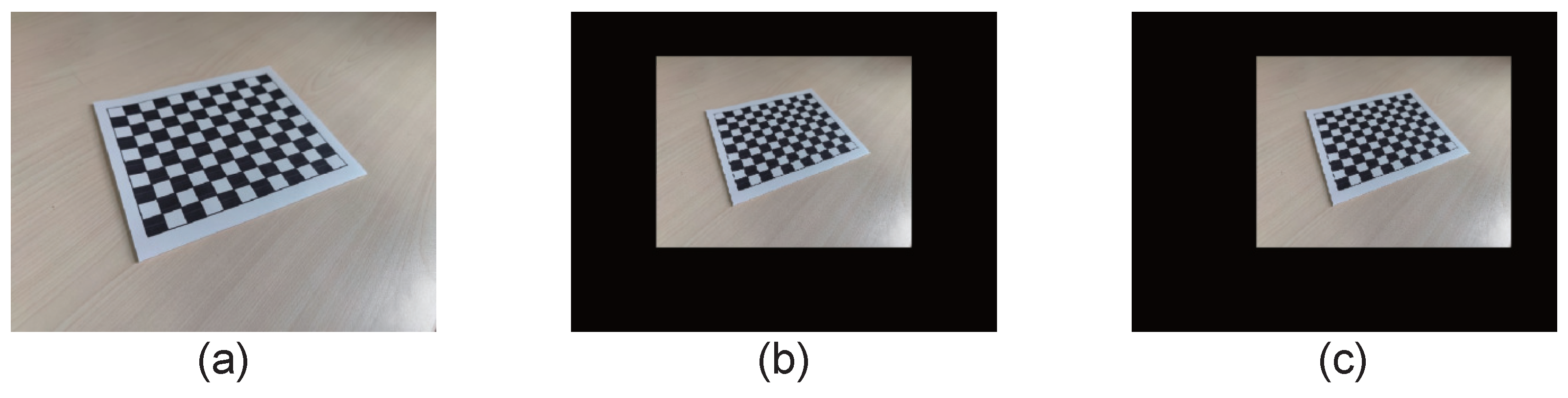
- Scaling
- (2)
- Translation
- (3)
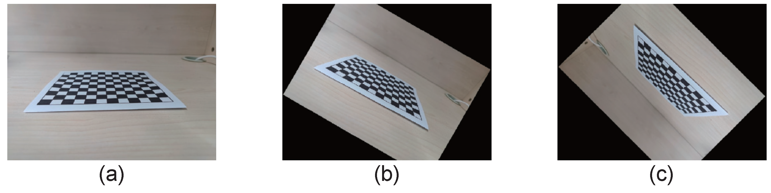
- Tilt correction
- (4)
- BEV
4.1.2. Verify on FPGA
4.2. Analysis of Performance

| Design | [18] | [19] | [20] | [21] | ||
|---|---|---|---|---|---|---|
| Function | OD 1 and PT 2 | BEV | PT | BEV/PT | BEV/PT | BEV/PT |
| WSRCP 3 | No | Yes | Yes | Yes | No | No |
| Platform | ASIC | Zynq-7000 | Stratix III | Virtex 6 | Zynq-7000 | Zynq-7000 |
| LUTs | 30,000 | 2280 | 6987 | 2983 | 2893 | 11,223 |
| Registers | - 4 | - | 7922 | 5684 | 1376 | 5821 |
| BRAM | - | 4 | - | 0 | 0 | 0 |
| DSP | - | 37 | 128 | 9 | 8 | 64 |
| Video Resolution | HD 5 (FHD 6) | VGA 7 | FHD | VGA | VGA | VGA |
| Maximum frequency | 140 MHz | 100 MHz | 74.25 MHz | - | 215.8 MHz | 212.2 MHz |
| Maximum frame rate | 60 Hz | - | 30 Hz | 30 Hz | 20 Hz | 157 Hz |
5. Conclusions
Author Contributions
Funding
Conflicts of Interest
Abbreviations
| LUTs | Look-up Tables |
| ASIC | Application Specific Integrated Circuit |
| FPGA | Field Programmable Gate Array |
| BEV | Bird’s-Eye View |
| BRAM | Block Random Access Memory |
| DDR | Double Data Rate |
| IP | Intellectual Property |
| ROM | Read Only Memory |
| HDMI | High Definition Multimedia Interface |
| UART | Universal Asynchronous Receiver/Transmitter |
| VGA | Video Graphic Array |
| FHD | Full High Definition |
| OD | Optical Distortion |
| PT | Perspective Transformation |
| WSRCP | Whether Software is Required to Calculate Parameters |
| HD | High Definition |
References
- Dick, K.; Tanner, J.B.; Green, J.R. To Keystone or Not to Keystone, that is the Correction. In Proceedings of the 2021 18th Conference on Robots and Vision (CRV), Burnaby, BC, Canada, 26–28 May 2021; pp. 142–150. [Google Scholar]
- Kim, T.H. An Efficient Barrel Distortion Correction Processor for Bayer Pattern Images. IEEE Access 2018, 6, 28239–28248. [Google Scholar] [CrossRef]
- Park, J.; Byun, S.C.; Lee, B.U. Lens distortion correction using ideal image coordinates. IEEE Trans. Consum. Electron. 2009, 55, 987–991. [Google Scholar] [CrossRef]
- Xu, Y.; Zhou, Q.; Gong, L.; Zhu, M.; Ding, X.; Teng, R.K. High-speed simultaneous image distortion correction transformations for a multicamera cylindrical panorama real-time video system using FPGA. IEEE Trans. Circuits Syst. Video Technol. 2013, 24, 1061–1069. [Google Scholar] [CrossRef]
- Yang, S.J.; Ho, C.C.; Chen, J.Y.; Chang, C.Y. Practical homography-based perspective correction method for license plate recognition. In Proceedings of the 2012 International Conference on Information Security and Intelligent Control, Yunlin, Taiwan, 14–16 August 2012; pp. 198–201. [Google Scholar]
- Chae, S.H.; Yoon, S.I.; Yun, H.K. A Novel Keystone Correction Method Using Camera—Based Touch Interface for Ultra Short Throw Projector. In Proceedings of the 2021 IEEE International Conference on Consumer Electronics (ICCE), Las Vegas, NV, USA, 10–12 January 2021; pp. 1–3. [Google Scholar]
- Kim, J.; Hwang, Y.; Choi, B. Automatic keystone correction using a single camera. In Proceedings of the 2015 12th International Conference on Ubiquitous Robots and Ambient Intelligence (URAI), Goyangi, Korea, 28–30 October 2015; pp. 576–577. [Google Scholar]
- Zhang, B.L.; Ding, W.Q.; Zhang, S.J.; Shi, H.S. Realization of Automatic Keystone Correction for Smart mini Projector Projection Screen. In Applied Mechanics and Materials; Trans Tech Publications: Zurich, Switzerland, 2014; Volume 519, pp. 504–509. [Google Scholar]
- Ye, Y. A New Keystone Correction Algorithm of the Projector. In Proceedings of the 2014 International Conference on Management of e-Commerce and e-Government, Shanghai, China, 31 October–2 November 2014; pp. 206–210. [Google Scholar]
- Li, Z.; Wong, K.H.; Gong, Y.; Chang, M.Y. An effective method for movable projector keystone correction. IEEE Trans. Multimed. 2010, 13, 155–160. [Google Scholar] [CrossRef]
- Jagannathan, L.; Jawahar, C. Perspective correction methods for camera based document analysis. In Proceedings of the First International Workshop on Camera-Based Document Analysis and Recognition, Seoul, Korea, 29 August 2005; pp. 148–154. [Google Scholar]
- Li, B.; Sezan, I. Automatic keystone correction for smart projectors with embedded camera. In Proceedings of the 2004 International Conference on Image Processing (ICIP’04), Singapore, 24–27 October 2004; Volume 4, pp. 2829–2832. [Google Scholar]
- Winzker, M.; Rabeler, U. Electronic distortion correction for multiple image layers. J. Soc. Inf. Disp. 2003, 11, 309–316. [Google Scholar] [CrossRef]
- Sukthankar, R.; Mullin, M.D. Automatic keystone correction for camera-assisted presentation interfaces. In International Conference on Multimodal Interfaces; Springer: Berlin/Heidelberg, Germany, 2000; pp. 607–614. [Google Scholar]
- Soycan, A.; Soycan, M. Perspective correction of building facade images for architectural applications. Eng. Sci. Technol. Int. J. 2019, 22, 697–705. [Google Scholar] [CrossRef]
- Zhang, W.; Li, X.; Ma, X. Perspective correction method for Chinese document images. In Proceedings of the 2008 International Symposium on Intelligent Information Technology Application Workshops, Shanghai, China, 21–22 December 2008; pp. 467–470. [Google Scholar]
- Miao, L.; Peng, S. Perspective rectification of document images based on morphology. In Proceedings of the 2006 International Conference on Computational Intelligence and Security, Guangzhou, China, 3–6 November 2006; Volume 2, pp. 1805–1808. [Google Scholar]
- Eo, S.W.; Lee, J.G.; Kim, M.S.; Ko, Y.C. Asic design for real-time one-shot correction of optical aberrations and perspective distortion in microdisplay systems. IEEE Access 2018, 6, 19478–19490. [Google Scholar] [CrossRef]
- Bilal, M. Resource-efficient FPGA implementation of perspective transformation for bird’s eye view generation using high-level synthesis framework. IET Circuits Devices Syst. 2019, 13, 756–762. [Google Scholar] [CrossRef]
- Hübert, H.; Stabernack, B.; Zilly, F. Architecture of a low latency image rectification engine for stereoscopic 3-D HDTV processing. IEEE Trans. Circuits Syst. Video Technol. 2012, 23, 813–822. [Google Scholar] [CrossRef]
- Botero, D.; Piat, J.; Chalimbaud, P.; Devy, M.; Boizard, J.L. Fpga implementation of mono and stereo inverse perspective mapping for obstacle detection. In Proceedings of the 2012 Conference on Design and Architectures for Signal and Image Processing, Karlsruhe, Germany, 23–25 October 2012; pp. 1–8. [Google Scholar]
- Rukundo, O.; Cao, H. Nearest neighbor value interpolation. Int. J. Adv. Comput. Sci. Appl. 2012, 3, 25–30. [Google Scholar]
- Blu, T.; Thévenaz, P.; Unser, M. Linear interpolation revitalized. IEEE Trans. Image Process. 2004, 13, 710–719. [Google Scholar] [CrossRef] [PubMed]
- Mastyło, M. Bilinear interpolation theorems and applications. J. Funct. Anal. 2013, 265, 185–207. [Google Scholar] [CrossRef]
- Huang, Z.; Cao, L. Bicubic interpolation and extrapolation iteration method for high resolution digital holographic reconstruction. Opt. Lasers Eng. 2020, 130, 106090. [Google Scholar] [CrossRef]
- Behjat, H.; Doğan, Z.; Van De Ville, D.; Sörnmo, L. Domain-informed spline interpolation. IEEE Trans. Signal Process. 2019, 67, 3909–3921. [Google Scholar] [CrossRef]
- Eberly, D. Perspective Mappings. Available online: https://www.geometrictools.com/Documentation/PerspectiveMappings.pdf (accessed on 1 April 2019).
- Barreto, J.P. A unifying geometric representation for central projection systems. Comput. Vis. Image Underst. 2006, 103, 208–217. [Google Scholar] [CrossRef][Green Version]
- Chen, M.; Zhang, Y.; Lu, C. Efficient architecture of variable size HEVC 2D-DCT for FPGA platforms. Aeu-Int. J. Electron. Commun. 2017, 73, 1–8. [Google Scholar] [CrossRef]
- Li, Z.; Wang, W.; Jiang, R.; Ren, S.; Wang, X.; Xue, C. Hardware Acceleration of MUSIC Algorithm for Sparse Arrays and Uniform Linear Arrays. IEEE Trans. Circuits Syst. Regul. Pap. 2022, 1–14. [Google Scholar] [CrossRef]
- Zhang, Y.; Lu, C. Efficient algorithm adaptations and fully parallel hardware architecture of H. 265/HEVC intra encoder. IEEE Trans. Circuits Syst. Video Technol. 2018, 29, 3415–3429. [Google Scholar] [CrossRef]
- Pastuszak, G.; Abramowski, A. Algorithm and architecture design of the H. 265/HEVC intra encoder. IEEE Trans. Circuits Syst. Video Technol. 2015, 26, 210–222. [Google Scholar] [CrossRef]


Publisher’s Note: MDPI stays neutral with regard to jurisdictional claims in published maps and institutional affiliations. |
© 2022 by the authors. Licensee MDPI, Basel, Switzerland. This article is an open access article distributed under the terms and conditions of the Creative Commons Attribution (CC BY) license (https://creativecommons.org/licenses/by/4.0/).
Share and Cite
Li, Z.; Wang, W.; Xue, C.; Jiang, R. Resource-Efficient Hardware Implementation of Perspective Transformation Based on Central Projection. Electronics 2022, 11, 1367. https://doi.org/10.3390/electronics11091367
Li Z, Wang W, Xue C, Jiang R. Resource-Efficient Hardware Implementation of Perspective Transformation Based on Central Projection. Electronics. 2022; 11(9):1367. https://doi.org/10.3390/electronics11091367
Chicago/Turabian StyleLi, Zeying, Weijiang Wang, Chengbo Xue, and Rongkun Jiang. 2022. "Resource-Efficient Hardware Implementation of Perspective Transformation Based on Central Projection" Electronics 11, no. 9: 1367. https://doi.org/10.3390/electronics11091367
APA StyleLi, Z., Wang, W., Xue, C., & Jiang, R. (2022). Resource-Efficient Hardware Implementation of Perspective Transformation Based on Central Projection. Electronics, 11(9), 1367. https://doi.org/10.3390/electronics11091367