Adversarial Attack and Defense: A Survey

Abstract

In recent years, artificial intelligence technology represented by deep learning has achieved remarkable results in image recognition, semantic analysis, natural language processing and other fields. In particular, deep neural networks have been widely used in different security-sensitive tasks. Fields, such as facial payment, smart medical and autonomous driving, which accelerate the construction of smart cities. Meanwhile, in order to fully unleash the potential of edge big data, there is an urgent need to push the AI frontier to the network edge. Edge AI, the combination of artificial intelligence and edge computing, supports the deployment of deep learning algorithms to edge devices that generate data, and has become a key driver of smart city development. However, the latest research shows that deep neural networks are vulnerable to attacks from adversarial example and output wrong results. This type of attack is called adversarial attack, which greatly limits the promotion of deep neural networks in tasks with extremely high security requirements. Due to the influence of adversarial attacks, researchers have also begun to pay attention to the research in the field of adversarial defense. In the game process of adversarial attacks and defense technologies, both attack and defense technologies have been developed rapidly. This article first introduces the principles and characteristics of adversarial attacks, and summarizes and analyzes the adversarial example generation methods in recent years. Then, it introduces the adversarial example defense technology in detail from the three directions of model, data, and additional network. Finally, combined with the current status of adversarial example generation and defense technology development, put forward challenges and prospects in this field.

1. Introduction

In recent years, deep neural network (DNN) has been widely used in computer vision [1,2,3], speech recognition [4,5,6], NLP [7,8] and many other fields, and has made great achievements in industrial the industry and academia have set off a wave of artificial intelligence represented by deep neural networks. Meanwhile, the combination of deep learning technology and edge computing has provided a strong drive for the development of smart cities. However, the security of deep neural network has not been scientifically explained and dealt with. The deep neural network obtains results through its own structure and algorithm mechanism, and relies on a large amount of external data during the training process. The features of the data determine the deep neural network. judgment result. Therefore, attackers can attack deep neural networks by modifying the data. As shown in Figure 1, after adding subtle perturbations to the original image, the human eye cannot detect the change in the image, but once it is input into the neural network model, it will seriously affect its recognition performance.

Szegedy et al. [9] first proposed the vulnerability of deep neural network models in image classification tasks. The adversarial examples generated after adding perturbation to the original image are indistinguishable to the human eye, but the deep neural network can output wrong results with high confidence. The recognition performance of the network is severely affected. As shown in Figure 2, after adding an adversarial perturbation to the original example to form an adversarial example, the target model incorrectly identifies “Cat” as “Dog”, and the human eye cannot detect the difference between the original example and the adversarial example. The white-box attack can obtain the structural information of the model, while the black-box attack can only obtain the output of the target model by inputting the original data to the target model. The attack strategy will be introduced together with the actual attack method. With the introduction of adversarial examples, researchers have begun to pay attention to the generation and defense methods of adversarial examples, and have achieved breakthrough results. This paper will discuss the methods of adversarial example generation and defense in computer vision in recent years. At present, there have been some reviews of countermeasures examples in the field of image. Compared with previous investigations, we have summarized and analyzed countermeasures attacks and focused on their generation principle. Meanwhile, this paper analyzes the defense technology from three aspects: model optimization, data optimization and additional network, so as to provide relevant reference for researchers in this field.

2. Adversarial Attack

In this section, we first introduce the characteristics and classification of adversarial attacks, and then analyze the typical adversarial attack methods based on the aggregated results.

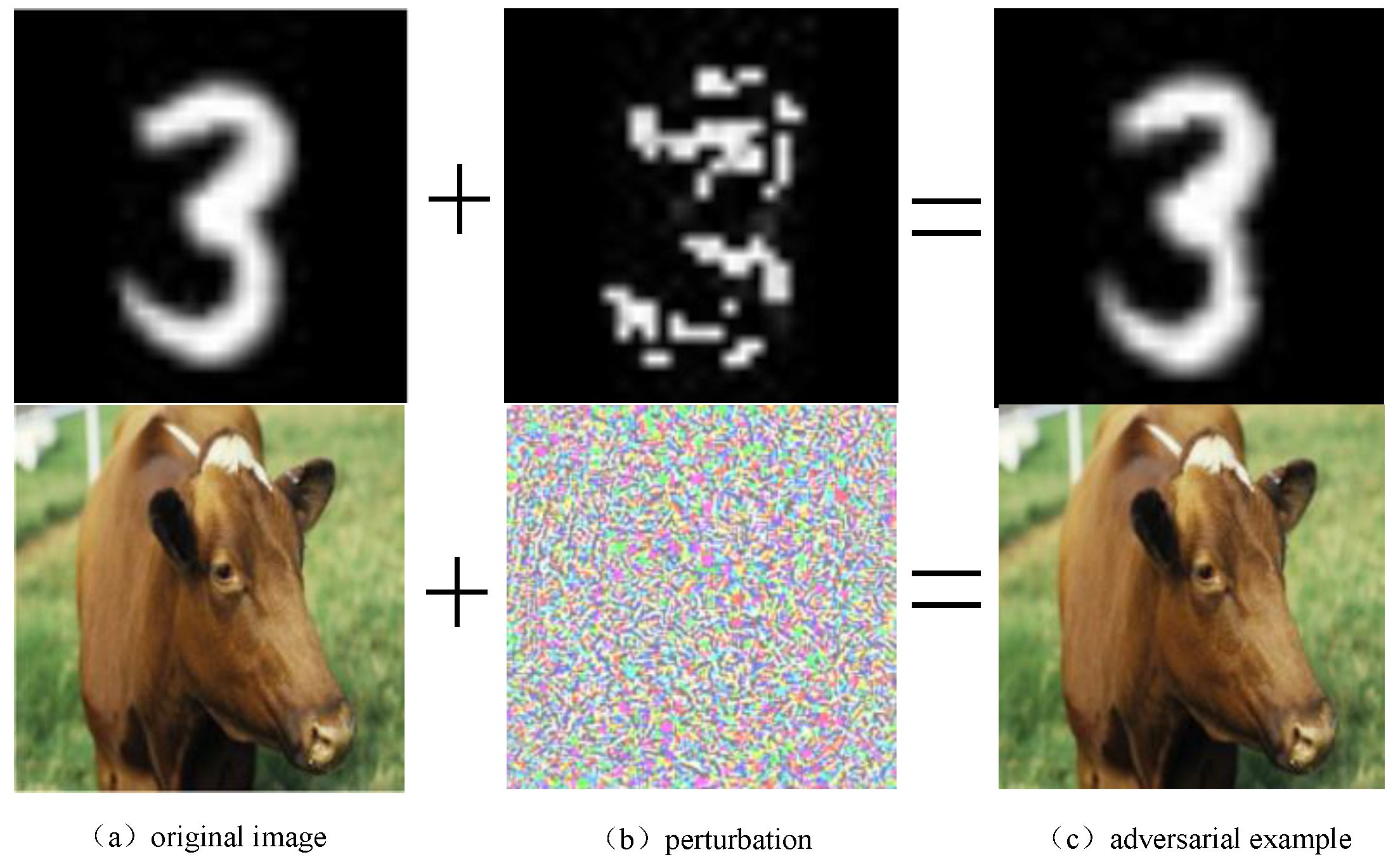
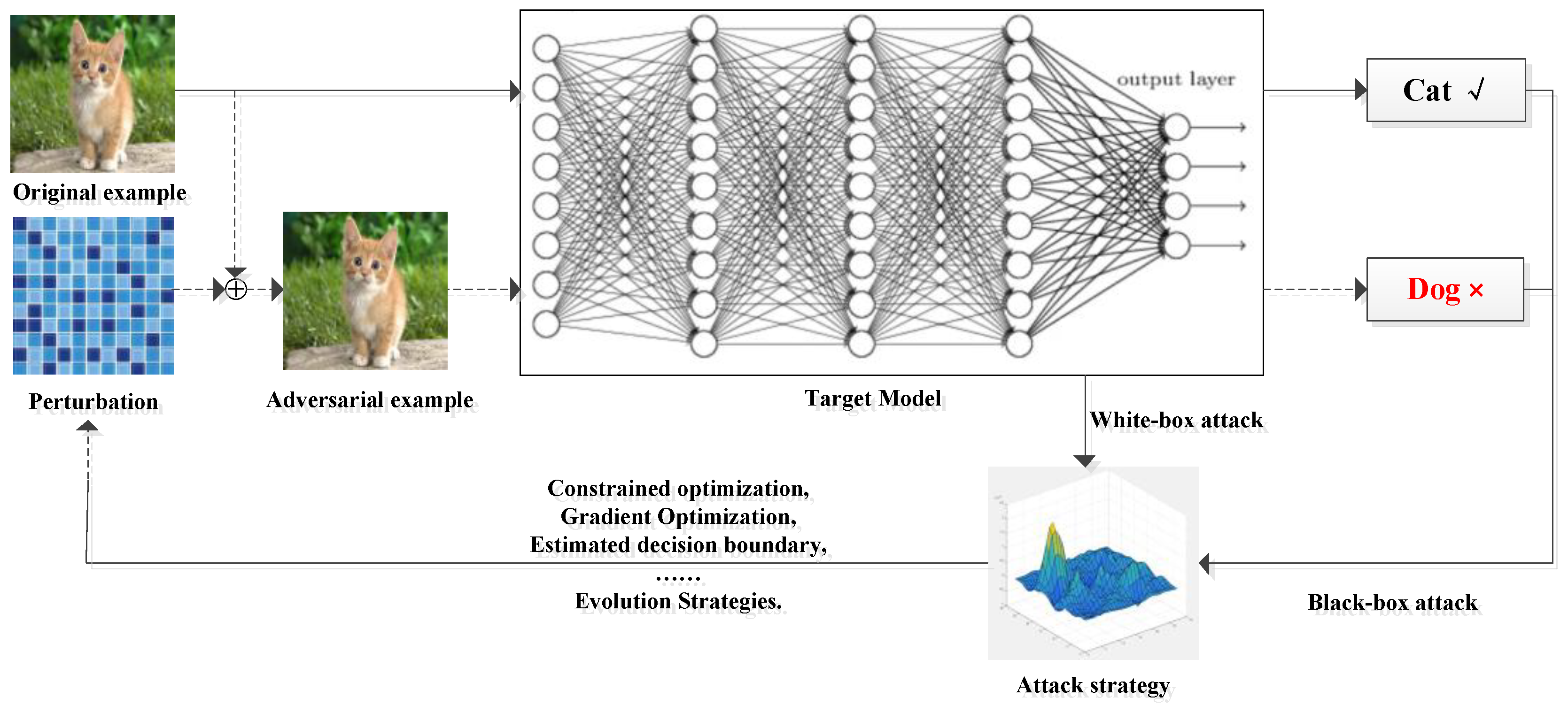
2.1. Common Terms

The adversarial attack is to attack the divine neural network through the adversarial example. According to the characteristics and attack effect of the adversarial attack, the adversarial attack can be divided into black-box attack and white-box attack, one shot attack and iterative attack, targeted attack and non-targeted attack, specific perturbation and universal perturbation, etc., the terms are introduced as follows:

Black-box attack: The attacker cannot access the deep neural network model, and thus cannot obtain the model structure and parameters, and can only obtain the output result of the target model by inputting the original data to the target model.

White-box attack: The attacker can obtain the complete structure and parameters of the target model, including training data, gradient information and activation functions, etc.

One-shot attack: The adversarial attack algorithm only needs to perform one calculation to obtain an adversarial example with a high attack success rate.

Iterative attack: The adversarial attack algorithm needs to be run multiple times to generate adversarial examples. Compared with the one-shot attack, iterative attack takes longer running time but has better attack effect.

Targeted attack: After the adversarial examples designed by the attacker are input into the target model, the target classifier can misjudge the specified classification result.

Non-targeted attack: The adversarial example only needs to be misjudged by the target classifier, and does not limit the classification result.

Specific perturbation: Add different perturbations to each input original data to form different perturbation patterns.

Universal perturbation: The same perturbation is added to each input original data, and its perturbation mode is the same.

2.2. Adversarial Attacks

At present, the academic circle has not reached a unified conclusion on the generating principle of adversarial examples. Szegedy et al. [9] believe that adversarial examples exist in real data, but the probability of occurrence is low, which makes it difficult for the model to learn adversarial examples. Therefore, after adversarial examples appear in the test set, it is difficult for the classifier to correctly identify the adversarial examples. While Goodfellow et al. [10] believe that the vulnerability of neural networks is due to the high-dimensional linear features of the model, when the model uses linear activation functions such as Relu or Maxout, it is more vulnerable to adversarial examples. Although the generation principle of adversarial examples has not been scientifically explained, in recent years, researchers have provided a theoretical and practical basis for improving the security of deep neural networks by exploring adversarial example generation algorithms. As shown in

Table 1. Summary of typical adversarial attack and its principle.

Adversarial Attacks	Attack Type	Attack Target	Attack Frequency	Perturbation Type	Perturbation Norm	Attack Strategy
L-BFGS [9]	White-box	Targeted	One-shot	Specific	$l_{\infty }$	Constrained optimization
FGSM [10]	White-box	Targeted	One-shot	Specific	$l_{\infty }$	Gradient optimization
JSMA [11]	White-box	Targeted	Iterative	Specific	$l_2$	Sensitivity analysis
C&W [12]	White-box	Targeted	Iterative	Specific	$l_0$ $l_2$ $l_{\infty }$	Constrained optimization
One-Pixel [13]	Black-box	Non-targeted	Iterative	Specific	$l_0$	Estimated decision boundary
DeepFool [14]	White-box	Non-targeted	Iterative	Specific	$l_0$ $l_2$ $l_{\infty }$	Gradient optimization
ZOO [15]	Black-box	Targeted	Iterative	Specific	$l_2$	Migration mechanism
UAP [16]	White-box	Non-targeted	Iterative	Universal	$l_2$ $l_{\infty }$	Gradient optimization
AdvGAN [17]	White-box	Targeted	Iterative	Specific	$l_2$	Generative model
ATNs [18]	White-box	Targeted	Iterative	Specific	$l_{\infty }$	Generative model
UPSET [19]	Black-box	Targeted	Iterative	Universal	$l_{\infty }$	Gradient approximation
ANGRI [19]	Black-box	Targeted	Iterative	Specific	$l_{\infty }$	Gradient approximation
Houdini [20]	Black-box	Targeted	Iterative	Specific	$l_2$ $l_{\infty }$	Constrained optimization
BPDA [21]	Black-box	Targeted	Iterative	Specific	$l_2$ $l_{\infty }$	Gradient approximation
DaST [22]	Black-box	Targeted	Iterative	Specific	$l_{\infty }$	Generative model
GAP++ [23]	White-box	Targeted	One-shot	Universal	$l_0$ $l_2$ $l_{\infty }$	Generative model
CG-ES [24]	Black-box	Targeted	Iterative	Specific	$l_0$ $l_2$ $l_{\infty }$	Evolution Strategies

, this paper summarizes and analyzes the current typical adversarial example generation methods based on attack type, attack target, attack frequency, perturbation type, perturbation norm, attack strategy, etc.

2.2.1. L-BFGS

Szegedy et al. [9] proposed that vulnerability of pairs to specific perturbations would lead to serious deviation of model recognition results in their exploration of the explainable work of deep learning. They proposed the first anti-attack algorithm for deep learning, L-BFGS:

$$\begin{array}{l}\min \hspace{0.17em}c\Vert \delta \Vert +{\mathrm{J}}_{\theta }(x^{\prime },l^{\prime })\\ s.t.\hspace{0.17em}{x}^{\prime }\in [0,1]\end{array},$$

(1)

where $c$ denotes a constant greater than 0, $x^{\prime }$ denotes the adversarial example formed by adding perturbation $\delta$ to the example, and ${\mathrm{J}}_{\theta }$ denotes the loss function. The algorithm is limited by the selection of parameter $c$, so it is necessary to select the appropriate $c$ to solve the constrained optimization problem. L-BFGS can be used in models trained on different datasets by virtue of its transferability. The proposal of this method has set off a research upsurge of scholars on adversarial examples.

2.2.2. FGSM

Goodfellow et al. [10] proposed the Fast Gradient Sign Method (FGSM) algorithm to prove that the existence of adversarial examples is caused by the high-dimensional linearity of deep neural networks. The algorithm principle is to generate adversarial perturbations according to the maximum direction of the gradient change of the deep learning model and add the perturbations to the image to generate adversarial examples. The formula for FGSM to generate perturbation is as follows:

$$\delta =\epsilon \mathrm{sign}({\nabla }_x{\mathrm{J}}_{\theta }(\theta ,x,y)),$$

(2)

where $\delta$ represents the generated perturbation; $\theta$ and $x$ are the parameters of the model and the input to the model, respectively; $y$ denotes the target associated with $x$; ${\mathrm{J}}_{\theta }$ is the loss function during model training. $\epsilon$ denotes a constant, when $\epsilon$ is 0.25, FGSM results in the shallow softmax classifier with a classification error rate of 99.9% and an average confidence rate of 79.3% on the MNIST dataset

The advantage of the FGSM algorithm is that the attack speed is fast, because the algorithm belongs to a single-step attack, but sometimes the attack success rate of the adversarial examples generated by the single-step attack is low. Therefore, Kurakin et al. [25] proposed an iteration-based FGSM (I-FGSM). The main innovation of I-FGSM is to generate perturbations by increasing the loss function in multiple small steps, so that more adversarial examples can be obtained.

2.2.3. JSMA

Papernot et al. [11] proposed the jacobian-based saliency map attack (JSMA). Instead of using the gradient information of the loss function output by the model, JSMA uses the probability information of the model output category to perform back-propagation to obtain the gradient information, and then build an adversarial saliency map to achieve the purpose of attack. The forward derivative of the deep learning model to the input example $x$ is as follows:

$$\nabla \mathrm{F}(x)=\frac{\partial \mathrm{F}(x)}{\partial x}={[\frac{\partial {\mathrm{F}}_j}{\partial x_i}]}_{i\ast j},$$

(3)

The degree of influence of each pixel point on model classification can be obtained through the forward gradient. Then, in order to quantify the influence of the change of pixel value on the target classifier, JSMA proposed the construction of adversarial significance graph based on Jacobian matrix, as shown below:

$$\mathrm{S}(x,t)[i]={\{}_{\frac{\partial {\mathrm{F}}_t(x)}{\partial x_i}\left|{\displaystyle \sum {}_{j\ne t}}\frac{\partial {\mathrm{F}}_t(x)}{\partial x_i}\right|,otherwise}^{0,\frac{\partial {\mathrm{F}}_t(x)}{\partial x_i}<0\hspace{0.17em}or\hspace{0.17em}{\displaystyle \sum {}_{j\ne t}}\frac{\partial {\mathrm{F}}_t(x)}{\partial x_i}>0},$$

(4)

where $i$ represents the input feature. The above formula can be used to calculate which pixel position changes can have the greatest impact on the target classification $t$. When $i$ is larger, the target classifier is more sensitive to the perturbation of this feature. Therefore, JSMA chooses the one with the largest anti-significant value. Pixels are perturbed to generate adversarial examples. The author proves through experiments that when 4.02% of the features in the example are changed, the JSMA attack can obtain an attack effect with a confidence rate of 97%. Moreover, the perturbation value calculated by this method is relatively small, so the change to the example is difficult to be recognized by the human eye.

2.2.4. C&W

In response to the attack methods proposed by scholars, Papernot et al. [26] proposed defensive distillation, which uses the distillation algorithm [27] to transfer the knowledge of the complex network to the simple network, so that the attacker cannot directly contact the original model to attack, Defensive distillation effectively defends against some adversarial examples. For defensive distillation, Carlini et al. [12] proposed a C&W attack by constraining $l_0$, $l_2$ and $l_{\infty }$. Experiments show that defensive distillation cannot defend against C&W attacks, and the general perturbation constraints of C&W attacks are as follows:

$$\begin{array}{l}\mathrm{minimize}\hspace{0.17em}\mathrm{D}(x,x+\delta )+c\cdot \mathrm{f}(x+\delta )\\ \mathrm{such}\hspace{0.17em}\mathrm{that}\hspace{0.17em}x+\delta \in {[0,1]}^n\end{array},$$

(5)

where D represents constraint paradigms such as $l_0$, $l_2$ and $l_{\infty }$, $l_0$ constraint the number of clean example points changed in the generation process, $l_2$ constraint the overall degree of perturbation, $l_{\infty }$ constraint the maximum allow perturbed per pixel, $c$ denotes the hyperparameter, and $\mathrm{f}$ adopts a variety of objective functions. By conducting experiments on the MINIST and CIFAR datasets, C&W achieves an attack on the distillation network with a 100% success rate, and C&W can generate high-confidence adversarial examples by adjusting the parameters.

2.2.5. One-Pixel

Su et al. [13] proposed an attack method One-Pixel attack (OPA), which only needs to change one pixel to generate adversarial examples. This method uses differential evolution algorithm to find adversarial perturbations, and then changes one or a small number of pixels to cause the model to misclassify, the OPA attack formula is as follows:

$$\begin{array}{l}\mathrm{maximize}\hspace{0.17em}{f}_{adv}(x+\mathrm{e}(x))\\ \mathrm{subject}\hspace{0.17em}\mathrm{to}\hspace{0.17em}\Vert \mathrm{e}(x)\Vert \le d\end{array},$$

(6)

When $d$ = 1, it means that the network only changes one pixel of the model. The author uses the differential evolution algorithm to obtain the optimal adversarial perturbation of the attack effect. For the n-dimensional image $x=(x_1,\cdots ,x_n)$, the perturbation caused by changing one pixel is actually along the direction parallel to the n-dimension. The interference of data points is carried out in one direction. Each perturbation is a 5-tuple, including x coordinate, y coordinate and RGB value. The calculation formula is as follows:

$$\begin{array}{l}{\mathrm{x}}_i(g+1)={\mathrm{x}}_{r1}(g)+\mathrm{F}({\mathrm{x}}_{r2}(g)+{\mathrm{x}}_{r3}(g))\\ r_1\ne r_2\ne r_3\end{array},$$

(7)

where $x_i$ denotes the candidate solution, $r_1$, $r_2$, $r_3$ are random numbers, $\mathrm{F}$ represents the scale parameter, which is set to 0.5, and $g$ is the current iteration number. After each iteration, if the result obtained by the candidate solution exceeds the parent result, then the candidate solution continues to the next iteration, otherwise, the parent result proceeds to the next iteration until the best attack result is obtained or the maximum number of iterations is reached.

2.2.6. DeepFool

Moosavi-Dezfooli et al. [14] proposed a method DeepFool based on gradient iteration to generate adversarial perturbations. DeepFool first obtains perturbations by calculation, and then pushes normal examples to the decision boundary through continuous iterative pixel adjustment until the adversarial examples are obtained after crossing the decision boundary. Taking binary classification as an example, assuming that the classification function is $\mathrm{f}(x)=w^{T}x+b$, the corresponding affine plane is $\beta =\{x:w^T+b=0\}$. Therefore, the minimum perturbation $\delta$ that affects the classification result of the original example $x_0$ by the classification function is equal to the orthogonal projection of $x_0$ to $\beta$, and the calculation formula of $\delta$ is as follows:

$$\begin{array}{l}{\delta }_{*}(x_0):=\arg \min {\Vert \delta \Vert }_2\\ s.t.\hspace{0.17em}\mathrm{sign}(\mathrm{f}(x_0+\delta ))\ne \mathrm{sign}(\mathrm{f}(x_0))\\ =-\frac{\mathrm{f}(x_0)}{{\Vert w\Vert }_2^2}w\end{array},$$

(8)

The above objective function solves the minimum adversarial perturbation $\delta$ in an iterative manner, and the calculation formula is as follows:

$$\begin{array}{l}\arg \min {\Vert {\delta }_i\Vert }_2\\ s.t.\hspace{0.17em}\mathrm{f}(x_i)+\nabla \mathrm{f}{(x_i)}^T{\delta }_i=0\end{array},$$

(9)

DeepFool measures the robustness of examples by computing the minimum distance between the decision boundary of normal examples and adversarial examples. Meanwhile, c compared with the single-step attack on FGSM, DeepFool can generate more accurate perturbations in a shorter time, but Deepfool can only achieve non-targeted attack.

2.2.7. ZOO

Different from some existing black-box attack methods based on surrogate models, Chen et al. [15] proposed the zeroth order optimization (ZOO), which does not exploit the attack transferability of surrogate models, but It is to estimate the value of the first-order gradient and the second-order gradient, and then use Adma or Newton’s method to iterate to obtain the optimal adversarial example, and add a perturbation to a given input $x:x=x+h{e}_i$, where $h$ is a small constant, $e_i$ represents a vector where i-th is 1 and the rest are 0. The first-order estimated gradient value is calculated as follows:

$${\widehat{g}}_i:=\frac{\partial \mathrm{f}(x)}{\partial x_i}\approx \frac{\mathrm{f}(x+h{e}_i)-\mathrm{f}(x-h{e}_i)}{2h},$$

(10)

The second-order estimated gradient is calculated as follows:

$${\widehat{h}}_i:=\frac{{\partial }^2\mathrm{f}(x)}{{\partial }^2{x}_{ii}}\approx \frac{\mathrm{f}(x+h{e}_i)-2\mathrm{f}(x)+\mathrm{f}(x-h{e}_i)}{h^2},$$

(11)

Chen et al. verified by experiments on the MNIST and CIFAR10 datasets that the ZOO attack can achieve a high attack success rate, but compared with the white-box attack C&W, the ZOO attack takes more time.

2.2.8. UAP

Moosavi-Dezfooli et al. [16] proposed a universal adversarial perturbations attack (UAP) based on DeepFool, which also uses adversarial perturbations to push normal examples to the decision boundary to form adversarial examples. It is defined as follows:

$$\widehat{\mathrm{k}}(x+\delta )\ne \widehat{\mathrm{k}}(x)\hspace{0.17em}for\hspace{0.17em}“most”\hspace{0.17em}x\sim \mu ,$$

(12)

where the general adversarial perturbation satisfies $\delta$ the following constraints:

$$\begin{array}{l}{\Vert \delta \Vert }_p\le \epsilon \\ P_{x~\mu }(\widehat{\mathrm{k}}(x+\delta )\ne \widehat{\mathrm{k}}(x))\ge 1-\theta \end{array},$$

(13)

where $\widehat{\mathrm{k}}(x)$ represents the classification function, $\epsilon$ parameter is used to control the strength of the adversarial perturbation $\delta$, and $\theta$ is used to control the success rate of the attack on the original example. In the iterative process of UAP, the minimum perturbation of each example is obtained through the DeepFool algorithm and continuously updated. until the optimal adversarial example is generated. UAP attack achieves the purpose of transplanting locally generated adversarial perturbations to the target network for attack. Although Moosavi-Dezfooli et al. only conducted experiments on ResNet to verify the effectiveness of general perturbation, the UAP attack has been successfully generalized to other neural networks.

2.2.9. advGAN

Xiao et al. [17] proposed an adversarial attack method advGAN based on generative adversarial network, which is mainly composed of generator $\mathrm{G}$, discriminator $\mathrm{D}$ and target network model $\mathrm{C}$. AdvGAN first inputs original example $x$ into generator to generate adversarial perturbation $\mathrm{g}(x)$, and then inputs $x+\mathrm{g}(x)$ into discriminator and target model, respectively. On the one hand, discriminator $\mathrm{D}$ is used to identify the category of examples. The target function of AdvGAN is shown as follows:

$$\mathrm{L}={\mathrm{L}}_{adv}+\alpha {\mathrm{L}}_{GAN}+\beta {\mathrm{L}}_{hinge},$$

(14)

The objective function is divided into three parts, where ${\mathrm{L}}_{adv}$ is the misjudgment loss, the purpose is to guide the generator to generate the best adversarial perturbation, and its formula is as follows:

$${\mathrm{L}}_{adv}={\mathrm{E}}_x{\mathrm{l}}_C(x+\mathrm{g}(x),t),$$

(15)

The adversarial perturbations generated by AdvGAN can guide the model to misclassify it as class $t$. ${\mathrm{L}}_{GAN}$ denotes the adversarial loss, that is, the original loss function proposed by GoodFellow. The formula is as follows:

$${\mathrm{L}}_{GAN}={\mathrm{E}}_x\log \mathrm{D}(x)+{\mathrm{E}}_x\log (1-\mathrm{D}(x+\mathrm{g}(x))),$$

(16)

The goal of this loss function is to optimize the generator $\mathrm{G}$ and the discriminator $\mathrm{D}$. After training and optimization, the generator $\mathrm{G}$ can generate the best adversarial perturbation $\mathrm{g}(x)$, and the discriminator $\mathrm{D}$ can also efficiently identify adversarial examples. For the training of stable GAN, the formula is as follows:

$${\mathrm{L}}_{hinge}={\mathrm{E}}_x\max (0,{\Vert \mathrm{g}(x)\Vert }_2-c),$$

(17)

The hyperparameter $c$ denotes the optimized distance, and advGAN conducts black-box attack experiments on the MNIST dataset, achieving a success rate of 92.76%.

2.2.10. ATNs

Baluja et al. [18] proposed Adversarial Transformation Networks (ATNs) based on the generative model. The ATNs input is the original example, and the adversarial example is generated by training a feedforward neural network. On the one hand, it satisfies the minimum perturbation and maintains the similarity between the adversarial example and the original example, on the other hand, it satisfies the success rate of adversarial attacks. Therefore, the objective function is as follows:

$$\underset{\theta }{\arg \min }{\displaystyle \sum _{x_i\in X}\beta {\mathrm{L}}_X}(G_{F,\theta }(x_i),x_i)+{\mathrm{L}}_Y(\mathrm{F}(G_{\mathrm{F},\theta }(x_i)),\mathrm{F}(x_i)),$$

(18)

where ${\mathrm{G}}_{F,\theta }(x_i)$ represents the generative model that needs to be trained. After inputting the original example, the adversarial example is output. $\mathrm{F}(x_i)$ represents the attacked target model, where ${\mathrm{L}}_X$ and ${\mathrm{L}}_Y$ represent the loss function of the input space and the output space, respectively. The former is used to constrain the difference between the adversarial example and the original example. Similarity, the latter is used to constrain the success rate of adversarial attacks.

2.2.11. UPSET and ANGRI

Sarkar et al. [19] proposed two black-box attack methods, UPSET and ANGRI, the former generates generic perturbations for the target class and the latter generates image specific perturbations. UPSET generates an adversarial perturbation $\mathrm{R}$ through the residual generation network. Assuming that $t$ is the selected target category, the perturbation is expressed as $r_t=\mathrm{R}(t)$.The adversarial example generation formula is as follows:

$$x^{\prime }=\mathrm{U}(x,t)=\max (\min (s\times \mathrm{R}(t)+x,1)-1),$$

(19)

where $\mathrm{U}$ represents the UPSET network, and $\mathrm{s}$ is the size used to adjust the perturbation $r_t$. The loss function of the UPSET network consists of two parts, as follows:

$$\begin{array}{cc}\hfill \mathrm{L}\left(x,x^{\prime },t\right)& =\hspace{0.17em}{\mathrm{L}}_C(x^{\prime },t)+{\mathrm{L}}_F(x^{\prime },t)\hfill \\ & ={{\displaystyle {\sum }_{i=1}^m\log ({\mathrm{C}}_i(x^{\prime })[t])+w\Vert x^{\prime }-x\Vert }}_k^k\hfill \end{array}$$

(20)

where ${\mathrm{L}}_C$ penalizes the inability to generate the target attack class, and ${\mathrm{L}}_{\mathrm{F}}$ is used to ensure the similarity between the adversarial examples and the original examples. Compared with UPSRT, ANGRI concats $A_t$ and $A_x$ to obtain $A_c$, and then generates adversarial examples $x^{\prime }$. Since ANGRI can obtain input images, it can generate better adversarial images, even when the classifier is trained with noisy images, ANGRI can still generate better adversarial examples.

2.2.12. Houdini

Cisse et al. [20] proposed Houdini algorithm that could generate adversation examples for the final performance measurement of the tasks performed by the model for some combinative and non-decomsolvable problems that could not generate adversation examples through gradient descent, such as speech recognition and semantic segmentation. The loss function of the Houdini network is as follows:

$${\mathrm{L}}_H(\theta ,x,y)=P_{\gamma \sim N(0,1)}[{\mathrm{g}}_{\theta }(x,y)-{\mathrm{g}}_{\theta }(x,y^{\prime })<\gamma ]\cdot \mathrm{L}(y^{\prime },y)$$

(21)

where ${\mathrm{g}}_{\theta }$ represents the target neural network with parameter $\theta$, ${\mathrm{g}}_{\theta }(x,y)-{\mathrm{g}}_{\theta }(x,y^{\prime })$ represents the difference between the actual score and the predicted score, and $\mathrm{L}$ is the original loss function. In addition, Cisse et al. applied Houdini network to speech recognition, language segmentation and pose estimation, and achieved good performance.

2.2.13. BPDA

In order to verify that the defense based on gradient obfuscation is flawed, Athalye et al. [21] proposed backward pass differentiable approximation (BPDA). When a pre-trained classifier is given, a pre-processor $\mathrm{g}(\mathrm{x})$ is constructed, which satisfies $\mathrm{g}(\mathrm{x})\approx \mathrm{x}$, the derivative can be approximated as:

$${\nabla }_x\mathrm{f}(g(x)){|}_{x=x^{\prime }}\approx {\nabla }_x\mathrm{f}(x){|}_{x=\mathrm{g}(x^{\prime })},$$

(22)

BPDA can overcome the defense based on gradient confusion effectively through the above equation and acquire the approximate value of gradient, and then generate the counter example through the average value of several iterations. The authors carried out BPDA attacks against 7 defense models based on confounding gradient presented at ICLR2018. BPDA completely avoided 6 defenses and partially avoided 1 defense. The BPDA algorithm proves that the defense method based on gradient obfuscation has specific and obvious defects.

2.2.14. DaST

In real-world tasks, pre-trained models are difficult to obtain. In this paper, Zhou et al. [22] proposed the data-free substitute training method (DaST) to obtain substitute models for adversarial black-box attacks without the requirement of any real data. To achieve this, DaST utilizes specially designed generative adversarial networks (GANs) to train substitute models. In particular, we design a multi-branch architecture and label-controlled loss for generative models to handle the uneven distribution of synthetic examples. The substitute model is then trained with synthetic examples generated by the generative model and then labeled by the attacked model. The task of the substitute model is to mimic the output of the target model. This is a game of two, where the target model can be seen as the referee. The loss function for this game can be written as:

$${\mathrm{L}}_D=\mathrm{d}(\mathrm{T}(\widehat{X}),\mathrm{D}(\widehat{X})),$$

(23)

where $\mathrm{d}(\mathrm{T}(\widehat{X}),\mathrm{D}(\widehat{X}))$ represents the metric to measure the output distance between substitute model $\mathrm{D}$ and target model $\mathrm{T}$. Update the generative model:

$${\mathrm{L}}_G=e^{-d(\mathrm{T},D)}+\alpha {\mathrm{L}}_C,$$

(24)

where ${\mathrm{L}}_C$ represents the label-controal loss, $\alpha$ is used to controls the weight of ${\mathrm{L}}_C$.

DaST is the first substitute model to train adversarial attacks without any real data. Attackers can use this method to train substitute models of adversarial attacks without collecting any real data. Zhou et al. attacked an online machine learning model on Microsoft Azure. Using their method, the remote model misclassified 98.35% of the antagonistic examples.

2.2.15. GAP++

In contrast with algorithms that only rely on input images to generate adversarial perturbations, Mao et al. [23], inspired by previous work [28], propose a novel general framework GAP++ based on GAP [29], which can infer targets based on input images and target labels Condition perturbation. Different from previous single-target attack models, this model performs target-conditioned attack by learning the relationship between attack targets and image semantics. GAP++ can generate all types of target perturbations using only one trained model. In the architecture of GAP++, each input image requires a corresponding target label as conditional information. However, in the case of non-targets, there is no conditional target label. Therefore, use the zero vector for off-target training as it does not affect the learning of the internal representation by concatenating zero tensors in the model. Extensive experiments on the MNIST and CIFAR10 datasets demonstrate that the method achieves better performance under a single-target attack model and a higher deception rate under a small perturbation norm. Although GAP++ borrows the network architecture and normalization tricks of the original GAP, it is lighter in performance than GAP and thus can be used for many attack tasks.

2.2.16. CG-ES

Standard evolution strategies (ES) algorithms can perform black-box attacks, where Gaussian distribution is widely adopted as the search distribution. However, it may not be flexible enough to capture different distributions of adversarial perturbations around different benign examples. Feng et al. [24] proposed a new evolution strategies approach (CG-ES) for searching distribution to solve the fractional black-box attack problem, based on conditional luminescence model and Gaussian distribution. CG-ES transforms Gaussian-distributed variables into another space through a conditional flow-based model to enhance the ability and flexibility to capture the inherent distribution of adversarial perturbations on benign examples. In addition, Feng et al. proposed to pre-train the c-Glow [30] model by approximating the energy-based model to the perturbation distribution of the alternative model. Then the pre-trained c-Glow model is initialized as the attack target model in ES. Therefore, the proposed CG-ES method makes use of both query-based and transport-based attack methods, and achieves higher attack success rate and higher attack efficiency.

2.3. Adversarial Attacks Comparison

L-BFGS is an early adversarial attack algorithm, which has inspired other attack algorithms. The adversarial examples generated by L-BFGS have good mobility and can be applied in many different types of neural network structures. Although JSMA has High attack success rate, but because its attack depends on the Jacobian matrix of the input example, and the Jacobian matrix of different examples is quite different, JSMA does not have transferability. FGSM only needs one iteration to acquire the adversarial perturbation, so the attack efficiency is higher, but the attack success rate is not as good as iterative attack algorithms such as PGD. Compared with FGSM, JSMA and other attacks, the adversarial disturbance generated by DeepFool attack is relatively small, but DeepFool does not have the ability of directed attack. UAP achieves better generalization ability based on the idea of DeepFool, realizes the ability of general attack across models and data sets, and provides technical support for attack requirements in real scenarios. One-Pixel achieves the purpose of the attack by modifying a single pixel. Compared with other algorithms, the generated adversarial examples are more deceptive, but they require multiple rounds of iterations for the optimal solution, so the attack efficiency is low. C&W attack has strong aggressiveness. Compared with L-BFGS, FGSM, DeepFool and other attack methods, C&W can successfully break the defense of defensive distillation, but sacrifice the attack efficiency. UPSET and ANGRI were proposed at the same time, but UPSET does not depend on the properties of the input data and can achieve general attacks. The latter cannot achieve general attacks because it depends on the properties of the input data during training. AdvGAN, DaST and GAP++ all use generative adversarial networks in the attack process. AdvGAN, DaST and GAP++ all use the generative adversarial network in the attack process, and the formed adversarial examples have a strong attack effect, because the adversarial examples generated by the game process of the generator and the discriminator are highly similar to the original examples.

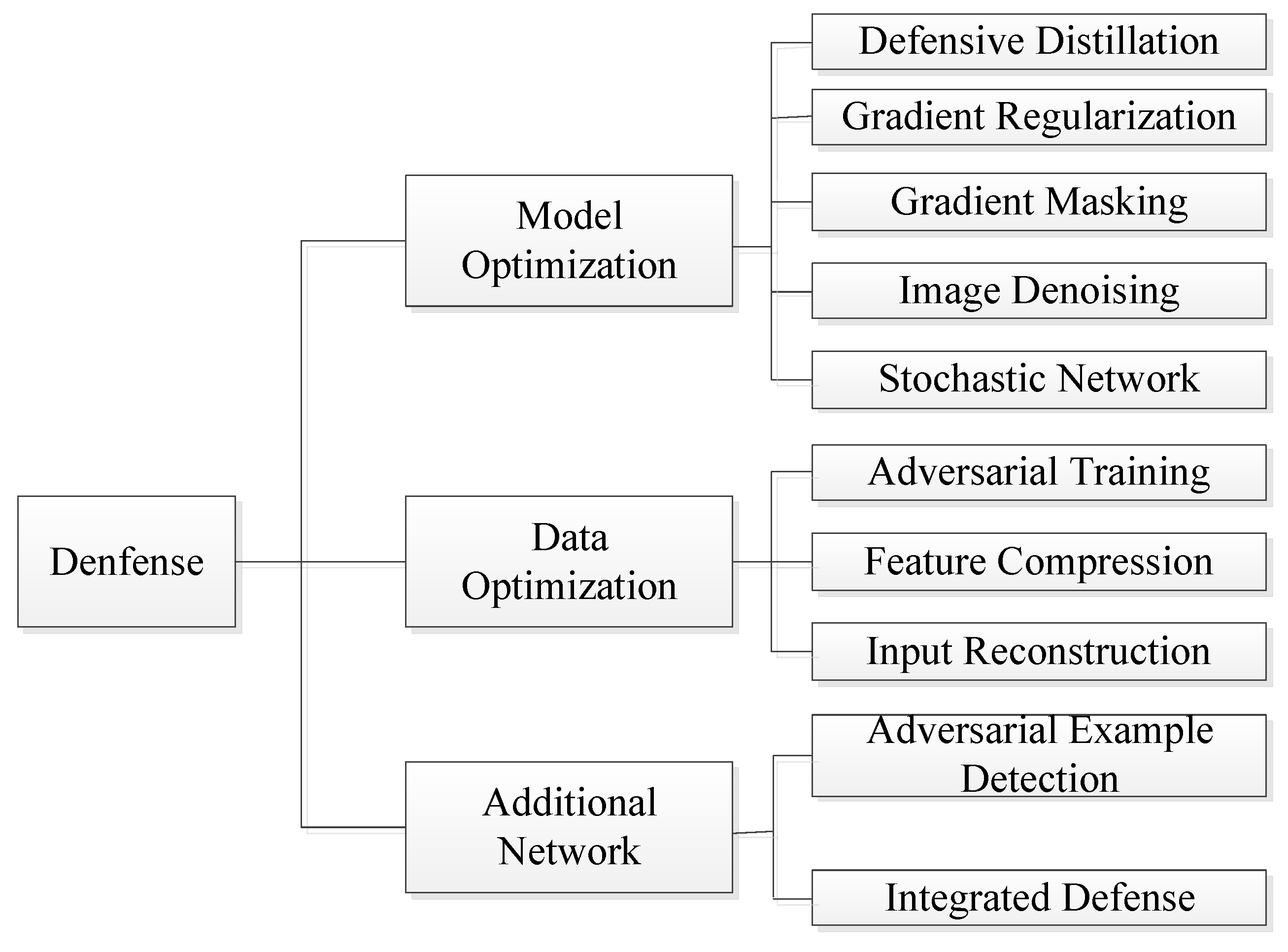
3. Adversarial Example Defense

We analyze the adversarial example defense from three directions: model optimization, data optimization and additional network. As shown in Figure 3, there are several specific technologies in each research direction. This section introduces defense technologies in different directions through some typical algorithms.

3.1. Model Optimization

3.1.1. Defensive Distillation

Distillation was first proposed by Hiton et al. [27], which is based on the idea of knowledge transfer to transfer complex networks to simple networks. In order to defend against adversarial attacks, Papernot et al. [26] proposed a defensive distillation technique. First, a distillation algorithm is used to train a distillation model for the original model. The input at this time is the original input example and label to obtain the probability distribution, and then use the input example and the probability distribution trains a distillation model with the same architecture to obtain a new probability distribution. At this point, the probability distribution is the new label, and the temperature T is a hyperparameter. When using the entire distillation network for classification tasks, it can effectively defend against adversarial attacks.

3.1.2. Gradient Regularization

Addepalli et al. [31] proposed a novel bit plane feature consistency (BPFC) regularizer that improves the adversarial robustness of the model by using the normal training mechanism. Forms a rough impression from the information in the higher bit planes and uses only the lower bit planes to refine its predictions. Experiments demonstrate that by imposing consistency on representations learned across different quantized images, the adversarial robustness of deep neural networks is significantly improved compared to normally trained models. The method is not due to the robustness achieved by gradient masking, but due to the improved local properties of the BPFC regularizer, which in turn yields better adversarial robustness.

Adversarial training requires additional sufficient data to ensure that the model is robust enough. Ma et al. [32] proposed second-order adversarial regularizer (SOAR) to replace adversarial training. In order to derive the regularizer, Ma et al. gave the adversarial robustness problem under the robust optimization framework, approximated the SOAR input with the second-order Taylor series of the loss function w.r.t., and approximately solved the inner maximization of the robust optimization formulation. Extensive experiments on both CIFAR-10 and SVHN datasets demonstrate that SOAR significantly improves the robustness of the network to $l_{\infty }$ and $l_2$ bounded perturbations generated by cross-entropy-based PGD [33].

3.1.3. Gradient Masking

In order to prevent attackers from attacking the model through gradient information, Folz et al. [34] proposed a defense method in which S2SNet masks the model gradient. S2SNet first converts the category-related information into structural information to influence the information in the gradient, and then encodes the structural parts required for the classification task, discarding other parts to eliminate adversarial perturbations. S2SNet preserves structural information through unsupervised training of encoder and decoder. Therefore, the resulting decoder directs attention to feature information that is highly relevant to the classification task, and then uses the gradient of the target model to fine-tune the decoder. During the entire training process, there is no class-related information involved in the gradient, so gradient-based adversarial examples cannot attack the model.

3.1.4. Image Denoising

The generation of adversarial examples is generated by adding specific noise to the original examples, which can resist the attack of adversarial examples through image denoising, but ordinary denoisers have the problem of residual error amplification effect, which leads to the wrong results of model output. Therefore, Liao et al. [35] proposed a high-level representation guided denoiser (HGD), which uses the U-Net network as the denoising network, and adds the loss function to the features of the high-level network, thereby suppressing the amplification of errors, The HGD loss function is as follows:

$$L=\Vert f_l(x^{\prime })-f_l(x)\Vert ,$$

(25)

When $l$ is −2, it is FGD, indicating the difference between the convolutional feature maps of the penultimate layer; when $l$ is −1 is LGD, indicating the difference between the convolutional feature maps of the last layer. Since FGD and LGD do not require label information of examples, they belong to unsupervised learning. Different from the previous two, CGD requires example tag information and requires the CNN model to predict a result and compare it with the tag. The HGD model can significantly defend against attacks against examples through denoising, and won the defense project champion of NIPS2017 offense and defense competition.

3.1.5. Stochastic Network

Wang et al. [36] provide a new solution to hardening DNNs under adversarial attacks through defensive dropout. Dropout is a common tuning method to deal with the overfitting problem caused by limited training data. As a tuning method, in addition to using dropout during training to obtain the best test accuracy, Wang et al. also use dropout during testing to obtain a strong defense effect. Defensive dropout algorithms determine the optimal test dropout rate given the neural network model and the attacker’s strategy for generating adversarial examples.

Wang et al. [37] proposed the Defense efficiency score (DES) to evaluate the robustness-accuracy trade-off of different defense systems. In order to achieve DES, Wang et al. proposed hierarchical random switching (HRS), which protects neural networks through a novel randomization scheme. HRS protection network consists of chain of random switching blocks. Each block contains a set of parallel channels with different weights, and a random switch that controls which channel is activated when the block’s input is received. At runtime, the input is only propagated through the activation channel of each block, and the activation channel is constantly switching. Each activation path in the HRS-protect model is characterized by decentralized randomization to improve robustness, in addition, in contrast with integrated defenses that use multiple different networks, HRS requires only a single underlying network architecture for defense. Compared with defensive dropout, experiments on MNIST and CIFAR-10 show that HRS achieves better defense effects at the expense of minimal test accuracy.

Liu et al. [38] proposed the random self-ensemble (RSE) defense method by adding a random noise layer to the neural network. The noise layer obtained by fusing the input vector with random noise is inserted before the convolutional layer of the neural network. Therefore, during training, the gradient is disturbed by the noise layer during the back-propagation calculation. In the inference phase, each time forward propagation, different prediction results will be obtained due to the existence of the noise layer, and then ensemble the results can effectively resist adversarial attacks. Taking CIFAR-10 data and VGG network as an example, the best defense technology in the past makes the classification accuracy of the model 48% when it is attacked by C&W. However, with RSE defense, the prediction accuracy of the model is 86.1%. In addition, the RSE training process ensures that the integration model can be well generalized and easily embedded into existing networks.

3.2. Data Optimization

3.2.1. Adversarial Training

Adversarial training is to add adversarial examples to the training set, and the feature distribution of the adversarial examples can be learned during model training, thereby increasing the robustness of the model. At present, adversarial training, as one of the main defense methods for adversarial examples, lacks research results on large-scale datasets, and various defense measures on ImageNet will be broken by specific white-box attacks. Therefore, Kannan et al. [39] introduced a logit pairing strategy based on PGD adversarial training [33] to propose mixed-minibatch PGD (M-PGD) adversarial training method. M-PGD adds clean examples to adversarial training, and the logit pairing strategy includes two pairing methods, one is pairing a clean example with an adversarial example, and the other is pairing a clean example with another clean example. The author verified on the ImageNet dataset that the adversarial logit pairing strategy has a certain ability to resist both white-box and black-box attacks. At this point, the defense of integrated adversarial training almost fails, and its accuracy rate is only 1.3%, while M-PGD’s accuracy rate under white-box attack and black-box attack is 27.9% and 47.1%, respectively.

Aiming at the problem that deep neural networks are vulnerable to physical attacks, Wu et al. [40] verified that PGD adversarial training [33] and random smoothing have limited robustness in two scenarios based on the eyeglass frame attack on face recognition and the sticker attack on stop signs. Therefore, they designed a novel defense against occlusion attacks (DOA) adversarial training defense method. First, an abstract adversarial model, rectangular occlusion attacks (ROA) is proposed. Compared with the traditional $l_p$-based model, ROA can better implement physical attacks. The ROA is used to place rectangular stickers on images to achieve attacks. Finally, adversarial examples are used for adversarial training. Experiments on adversarial eyeglasses in face recognition and adversarial stickers on stop signs prove that the DOA adversarial training model has strong robustness to physical attacks on deep neural networks.

3.2.2. Feature Compression

The perturbation between the adversarial example and the original image is very small, but is amplified in the high-dimensional space in the image classification model. Jia et al. [41] proposed an image compression-based adversarial example defense method ComDefend to eliminate redundant perturbations of images. ComDefend consists of a compression convolutional neural network (ComCNN) and a reconstruction convolutional neural network (RecCNN), where ComCNN compresses the 24-bit pixels of the input image into 12-bits to obtain a compressed representation of the original image, which can retain enough main information of the original image. The compressed representation is then input to ResCNN, which reconstructs the clean original image, and ResCNN adds Gaussian noise to the reconstruction process to improve the ability to resist adversarial examples. Compared with methods such as HGD, ComDefend does not require adversarial examples, thus reducing the computational cost. Meanwhile, ComDefend greatly improves the ability of deep neural networks to resist different adversarial attack methods, and its performance exceeds that of various defense models including the champion of the NIPS2017 adversarial attack and defense competition.

3.2.3. Input Reconstruction

In order to resist the attack of antagonistic examples, Guo et al. [42] proposed to eliminate image perturbation by using five image changes, including image clipping and rescaling, image depth reduction, JPEG compression, total variance minimization and image quilting, and maximize the retention of effective image information. Prakash et al. [43] proposed a method to redistribute pixel values based on pixel deflection to locally destroy the image, and use wavelet denoising technology to reduce the damage and adversarial perturbation caused by pixel offset, the classification results of clean examples are not affected, while the adversarial examples are correctly classified after pixel deflection, which achieves the purpose of eliminating perturbation.

Samangouei et al. [44] proposed an adversarial example defense method Defense-GAN based on WGAN [45]. First, a random noise generator was used to generate several random noise vectors, and then the random noise vectors were input to the generator together with the original examples. The training in the adversarial network ends when the random noise is fitted to the distribution of clean examples, and the above training process is repeated with the number of noise as the loop variable, and then the image with the best performance is selected for the classification task. Jin et al. [46] proposed an APE-GAN defense strategy, which also used the generator to reconstruct examples, but APE-GAN input the adversation examples and clean examples to the generator and discriminator for training, respectively, so as to eliminate adversation perturbations.

3.3. Additional Network

3.3.1. Adversarial Example Detection

Cohen et al. [47] proposed an adversarial attack detection method combining influence functions with KNN-based metrics. The method can be applied to any pretrained neural network to determine how data points in the training set affect the network’s decisions given a test example by using an influence function to measure the influence of each training example on the validation set data. The influence function measures the effect of a small weighting of a particular training point in the model’s loss function on the loss of the test point, providing a measure of how much the classification of the test example is affected by each training example. Meanwhile, KNN is used to search the ranking of these supporting training examples in the embedding space of DNN. It can be observed that these examples are highly correlated with the nearest neighbors of normal inputs, while the correlation of adversarial inputs is much weaker, which in turn detects adversarial examples.

Meng et al. [48] argue that the properties of adversarial examples should not be found from a specific generation process, but to enhance the generalization ability of defense methods by finding intrinsic common properties in the generation process of all adversarial examples. Therefore, Meng et al. propose an attack-independent defense framework, MagNet, which neither relies on adversarial examples and their generation process, nor modifies the original model, but only utilizes the features of the input data. MagNet is composed of Detector and Reformer. Based on the popular hypothesis of deep learning, the adversarial examples are located far from the popular boundary or the popular boundary. The function of the detector is to detect the confrontational examples far from the popular boundary, and refuse to classify them, and then reconstruct them through reconstruction. The classifier reconstructs the examples close to the popular boundary into the original examples for classification.

Previous adversarial example detection studies have shown that the input example and its neighbors exhibit significant consistency in the feature space. Based on this, Abusnaina et al. [49] proposed the Latent Neighborhood Graph (LNG) to characterize the neighborhood of input. In this paper, the problem of adversarial example detection is transformed into a Graph classification problem. Firstly, a Latent Neighborhood Graph is generated for each input example, and then a Graph neural network (GNN) is used to distinguish benign and adversarial examples by the relationship between nodes in the Neighborhood Graph. Given an input example, the selected reference adversarial and benign examples are used to capture local manifolds near the input example. LNG node connection parameters and graph Note network parameters are jointly optimized in an end-to-end manner to determine the optimal graph topology for adversarial example detection. The graph attention network is used to determine whether LNG is coming from an adversarial or benign input example.

Choi et al. [50] experimentally verified that malicious PowerShell files generated by GAN are difficult to be detected by traditional artificial intelligence algorithms, so they proposed an attention-based filtering method to detect malicious PowerShell. The method first uses the attention mechanism to generate a malicious token list from PowerShell training data, and then generates real PowerShell data from fake PowerShell data through the malicious token list. Experiments verify that the detection rate of PowerShell data restored based on attention filtering is 96.5%

3.3.2. Integrated Defense

In order to verify whether a strong adversarial defense capability can be constructed by integrating multiple weak defenses, He et al. [51] studied three ensemble defense methods, including feature compression, expert +1, and ensemble detection mechanism. In order to increase the credibility of the experiment, He et al. assume that the attacker is fully aware of the model’s architecture, parameters and defense strategies, by verifying on two datasets MNIST and CIFAR-10, when using adaptive attacks to evaluate these When defending, the attacker is able to defeat the above 3 integrated defenses with low distortion. Therefore, He et al. propose that when conducting adversarial defense research, robust attacks should be used to evaluate defense capabilities.

Yu et al. [52] proposed a novel defense method for AuxBlocks model, which extended the original model by introducing multiple AuxBlocks models similar to the self-ensemble model. Yu et al. divide the model into two parts: public model and private model, where the public model represents the original model, and the private model is several auxiliary models introduced. The public model can be exposed to the attacker, while the private model is private to the attacker, making it impossible for the attacker to generate valid adversarial examples. AuxBlocks are set up as miniature neural networks, which can also be any other structure. Yu et al. verified through experiments that the introduction of AuxBlocks into the neural network can effectively improve the robustness of the model. Even in response to adaptive white-box attacks, the auxiliary block model also shows strong defense capabilities.

4. Challenge

Adversarial attack and defense technologies have developed rapidly in the process of playing against each other. Researchers have proposed many cutting-edge algorithms. However, through surveys, it is found that there are still many challenges in adversarial attack and adversarial defense technologies that need to be tackled by researchers.

4.1. Adversarial Attack

(1)

Existing adversarial example generation models are all trained on specific datasets, lacking transferability, and need to verify the attack effect in real physical scenarios, such as security systems in smart cities, etc.

(2)

The computational complexity of some adversarial example generation techniques is too high. Although a relatively high attack success rate is achieved, it increases the amount of computation, resulting in an excessively large trained model. The adversarial example generation model cannot be transplanted into lightweight devices.

(3)

At present, adversarial attack technology is developing rapidly in the field of computer vision, but it is still in its infancy in the fields of NLP and speech recognition. It is necessary to increase the research on attack technology in these fields to provide theoretical and technical support to ensure that AI technology can play a safe and efficient role in the construction of smart city.

4.2. Adversarial Example Defense

(1)

For the vulnerability of deep neural networks, the academic community has not come up with a recognized scientific explanation, so it is impossible to fundamentally defend against the attack of adversarial examples;

(2)

The applicability and adaptability of adversarial example defense technology needs to be improved. Research has proved that even the defense technology with the best defense effect will be broken by an endless stream of adversarial attack technologies. How to improve the self-iteration capability of defense technology is an urgent problem to be solved.

(3)

The current defense technology research lacks the practice in the real world. How to convert the advanced defense theory and technology into the defense method in the physical scene is a major challenge for researchers.

5. Conclusions

Edge/urban IoT construction is inseparable from artificial intelligence technology, especially deep learning technology, but deep neural networks are vulnerable to adversarial attacks and cause serious errors. In order to secure the development of edge/urban IoT, in-depth research on adversarial example techniques is required. This paper conducts a comprehensive investigation and analysis on the attack and defense of adversarial examples in the field of computer vision. Due to the vulnerability of deep neural networks, once the adversarial examples are input, they will output wrong results with high confidence. This paper first introduces the types of adversarial attacks and the characteristics of adversarial example generation, and introduces, analyzes and compares typical adversarial example generation methods in recent years. Then, we introduce the state-of-the-art adversarial example defense techniques in detail from three research directions: model optimization, data optimization, and additional network. Finally, combined with the development of adversarial attack and defense technology, the challenges and opportunities existing in this stage are proposed.

References

- Zhou, L.; Xu, C.; Koch, P.; Corso, J.J. Watch What You Just Said: Image Captioning with Text-Conditional Attention. In Proceedings of the Thematic Workshops of ACM Multimedia, New York, NY, USA, 23–27 October 2017; pp. 305–313. [Google Scholar]
- You, Q.; Jin, H.; Wang, Z.; Fang, C.; Luo, J. Image captioning with semantic attention. In Proceedings of the IEEE Conference on Computer Vision and Pattern Recognition, Las Vegas, NV, USA, 27–30 June 2016; pp. 4651–4659. [Google Scholar]
- Lu, J.; Xiong, C.; Parikh, D.; Socher, R. Knowing when to look: Adaptive attention via a visual sentinel for image captioning. In Proceedings of the IEEE Conference on Computer Vision and Pattern Recognition, Honululu, HI, USA, 21–26 July 2017; pp. 375–383. [Google Scholar]
- Abdel-Hamid, O.; Mohamed, A.; Jiang, H.; Penn, G. Applying convolutional neural networks concepts to hybrid NN-HMM model for speech recognition. In Proceedings of the 2012 IEEE International Conference on Acoustics, Speech and Signal Processing (ICASSP), Kyoto, Japan, 27–29 March 2012; IEEE: New York, NY, USA, 2012; pp. 4277–4280. [Google Scholar]
- Kim, S.; Lane, I. Recurrent models for auditory attention in multi-microphone distance speech recognition. arXiv 2015, arXiv:1511.06407. [Google Scholar]
- Han, W.; Zhang, Z.; Zhang, Y.; Yu, J.; Chiu, C.C.; Qin, J.; Wu, Y. ContextNet: Improving Convolutional Neural Networks for Automatic Speech Recognition with Global Context. arXiv 2020, arXiv:2005.03191v3. [Google Scholar] [CrossRef]
- Yu, A.W.; Dohan, D.; Luong, T.; Zhao, R.; Chen, K.; Norouzi, M.; Le, Q.V. QANet: Combining Local Convolution with Global Self-Attention for Reading Comprehension. arXiv 2018, arXiv:1804.09541. [Google Scholar]
- Yin, W.; Schütze, H. Task-specific attentive pooling of phrase alignments contributes to sentence matching. arXiv 2017, arXiv:1701.02149. [Google Scholar]
- Szegedy, C.; Zaremba, W.; Sutskever, I.; Bruna, J.; Erhan, D.; Goodfellow, I.; Fergus, R. Intriguing properties of neural networks. arXiv 2013, arXiv:1312.6199. [Google Scholar]
- Goodfellow, I.J.; Shlens, J.; Szegedy, C. Explaining and Harnessing Adversarial Examples. arXiv 2014, arXiv:1412.6572. [Google Scholar]
- Papernot, N.; McDaniel, P.; Jha, S.; Fredrikson, M.; Celik, Z.B.; Swami, A. The limitations of deep learning in adversarial settings. In Proceedings of the 2016 IEEE European Symposium on Security and Privacy (EuroS&P), Las Vegas, NV, USA, 27–30 June 2016; IEEE: New York, NY, USA, 2016; pp. 372–387. [Google Scholar]
- Carlini, N.; Wagner, D. Towards evaluating the robustness of neural networks. In Proceedings of the 2017 IEEE Symposium on Security and Privacy (sp), Honululu, HI, USA, 21–26 July 2017; IEEE: New York, NY, USA, 2017; pp. 39–57. [Google Scholar]
- Su, J.; Vargas, D.V.; Sakurai, K. One pixel attack for fooling deep neural networks. IEEE Trans. Evol. Comput. 2019, 23, 828–841. [Google Scholar] [CrossRef] [Green Version]
- Moosavi-Dezfooli, S.M.; Fawzi, A.; Frossard, P. Deepfool: A simple and accurate method to fool deep neural networks. In Proceedings of the 2016 IEEE Conference on Computer Vision and Pattern Recognition (CVPR), Las Vegas, NV, USA, 27–30 June 2016; pp. 2574–2582. [Google Scholar]
- Chen, P.Y.; Zhang, H.; Sharma, Y.; Yi, J.; Hsieh, C.J. Zoo: Zeroth order optimization based black-box attacks to deep neural networks without training substitute models. In Proceedings of the 10th ACM Workshop on Artificial Intelligence and Security, Dallas, TX, USA, 3 November 2017; pp. 15–26. [Google Scholar]
- Moosavi-Dezfooli, S.M.; Fawzi, A.; Fawzi, O.; Frossard, P. Universal adversarial perturbations. In Proceedings of the IEEE Conference on Computer Vision and Pattern Recognition, Honululu, HI, USA, 21–26 July 2017; pp. 1765–1773. [Google Scholar]
- Xiao, C.; Li, B.; Zhu, J.Y.; He, W.; Liu, M.; Song, D. Generating adversarial examples with adversarial networks. arXiv 2018, arXiv:1801.02610. [Google Scholar]
- Baluja, S.; Fischer, I. Adversarial transformation networks: Learning to generate adversarial examples. arXiv 2017, arXiv:1703.09387. [Google Scholar]
- Sarkar, S.; Bansal, A.; Mahbub, U.; Chellappa, R. UPSET and ANGRI: Breaking high performance image classifiers. arXiv 2017, arXiv:1707.01159. [Google Scholar]
- Cisse, M.; Adi, Y.; Neverova, N.; Keshet, J. Houdini: Fooling deep structured prediction models. arXiv 2017, arXiv:1707.05373. [Google Scholar]
- Athalye, A.; Carlini, N.; Wagner, D. Obfuscated gradients give a false sense of security: Circumventing defenses to adversarial examples. In Proceedings of the International Conference on Machine Learning, PMLR, Stockholm, Sweden, 10–15 July 2018; pp. 274–283. [Google Scholar]
- Zhou, M.; Wu, J.; Liu, Y.; Zhu, C. Dast: Data-free substitute training for adversarial attacks. In Proceedings of the IEEE/CVF Conference on Computer Vision and Pattern Recognition, Seattle, WA, USA, 14–19 July 2020; pp. 234–243. [Google Scholar]
- Mao, X.; Chen, Y.; Li, Y.; He, Y.; Xue, H. Gap++: Learning to generate target-conditioned adversarial examples. arXiv 2020, arXiv:2006.05097. [Google Scholar]
- Feng, Y.; Wu, B.; Fan, Y.; Li, Z.; Xia, S. Efficient black-box adversarial attack guided by the distribution of adversarial perturbations. arXiv 2020, arXiv:2006.08538. [Google Scholar]
- Kurakin, A.; Goodfellow, I.; Bengio, S. Adversarial examples in the physical world. arXiv 2016, arXiv:1607.02533. [Google Scholar]
- Papernot, N.; McDaniel, P.; Wu, X.; Jha, S.; Swami, A. Distillation as a defense to adversarial perturbations against deep neural networks. In Proceedings of the 2016 IEEE Symposium on Security and Privacy (SP), San Jose, CA, USA, 22–26 May 2016; IEEE: New York, NY, USA, 2016; pp. 582–597. [Google Scholar]
- Hinton, G.; Vinyals, O.; Dean, J. Distilling the knowledge in a neural network. arXiv 2015, arXiv:1503.02531. [Google Scholar]
- Mao, X.; Chen, Y.; Li, Y.; Xiong, T.; He, Y.; Xue, H. Bilinear representation for language-based image editing using conditional generative adversarial networks. In Proceedings of the ICASSP 2019–2019 IEEE International Conference on Acoustics, Speech and Signal Processing (ICASSP), Brighton, UK, 12–17 May 2019; pp. 2047–2051. [Google Scholar]
- Poursaeed, O.; Katsman, I.; Gao, B.; Belongie, S. Generative adversarial perturbations. In Proceedings of the IEEE Conference on Computer Vision and Pattern Recognition, Salt Lake City, UT, USA, 18–22 June 2018; pp. 4422–4431. [Google Scholar]
- Lu, Y.; Huang, B. Structured output learning with conditional generative flows. In Proceedings of the AAAI Conference on Artificial Intelligence, New York, NY, USA, 7–12 February 2020; Volume 34, pp. 5005–5012. [Google Scholar]
- Addepalli, S.; Vivek, B.S.; Baburaj, A.; Sriramanan, G.; Babu, R.V. Towards achieving adversarial robustness by enforcing feature consistency across bit planes. In Proceedings of the IEEE/CVF Conference on Computer Vision and Pattern Recognition, Seattle, CA, USA, 14–19 June 2020; pp. 1020–1029. [Google Scholar]
- Ma, A.; Faghri, F.; Farahmand, A. Adversarial robustness through regularization: A second-order approach. arXiv 2020, arXiv:2004.01832. [Google Scholar]
- Madry, A.; Makelov, A.; Schmidt, L.; Tsipras, D.; Vladu, A. Towards Deep Learning Models Resistant to Adversarial Attacks. In Proceedings of the International Conference on Learning Representations, Vancover, BC, Canada, 27 November 2017–5 January 2018. [Google Scholar]
- Folz, J.; Palacio, S.; Hees, J.; Dengel, A. Adversarial defense based on structure-to-signal autoencoders. In Proceedings of the 2020 IEEE Winter Conference on Applications of Computer Vision (WACV), Snowmass Village, CO, USA, 1–5 March 2020; IEEE: New York, NY, USA, 2020; pp. 3568–3577. [Google Scholar]
- Liao, F.; Liang, M.; Dong, Y.; Pang, T.; Hu, X.; Zhu, J. Defense against adversarial attacks using high-level representation guided denoiser. In Proceedings of the IEEE Conference on Computer Vision and Pattern Recognition, Salt Lake City, UT, USA, 18–22 June 2018; pp. 1778–1787. [Google Scholar]
- Wang, S.; Wang, X.; Zhao, P.; Wen, W.; Kaeli, D.; Chin, P.; Lin, X. Defensive dropout for hardening deep neural networks under adversarial attacks. In Proceedings of the International Conference on Computer-Aided Design, Marrakesh, Morocco, 19–21 March 2018; pp. 1–8. [Google Scholar]
- Ang, X.; Wang, S.; Chen, P.Y.; Wang, Y.; Kulis, B.; Lin, X.; Chin, P. Protecting neural networks with hierarchical random switching: Towards better robustness-accuracy trade-off for stochastic defenses. arXiv 2019, arXiv:1908.07116. [Google Scholar]
- Liu, X.; Cheng, M.; Zhang, H.; Hsieh, C.J. Towards robust neural networks via random self-ensemble. In Proceedings of the European Conference on Computer Vision (ECCV), Tel-Aviv, Israel, 23–27 October 2018; pp. 369–385. [Google Scholar]
- Kannan, H.; Kurakin, A.; Goodfellow, I. Adversarial Logit Pairing. arXiv 2018, arXiv:1803.06373. [Google Scholar]
- Wu, T.; Tong, L.; Vorobeychik, Y. Defending against physically realizable attacks on image classification. arXiv 2019, arXiv:1909.09552. [Google Scholar]
- Jia, X.; Wei, X.; Cao, X.; Foroosh, H. Comdefend: An efficient image compression model to defend adversarial examples. In Proceedings of the IEEE/CVF Conference on Computer Vision and Pattern Recognition 2019, Long Beach, CA, USA, 15–20 June 2019; pp. 6084–6092. [Google Scholar]
- Guo, C.; Rana, M.; Cisse, M.; Van Der Maaten, L. Countering adversarial images using input transformations. arXiv 2017, arXiv:1711.00117. [Google Scholar]
- Prakash, A.; Moran, N.; Garber, S.; DiLillo, A.; Storer, J. Deflecting adversarial attacks with pixel deflection. In Proceedings of the IEEE Conference on Computer Vision and Pattern Recognition, Salt Lake City, UT, USA, 17–22 June 2018; pp. 8571–8580. [Google Scholar]
- Samangouei, P.; Kabkab, M.; Chellappa, R. Defense-GAN: Protecting Classifiers Against Adversarial Attacks Using Generative Models. In Proceedings of the International Conference on Learning Representations, Vancouver, BC, Canada, 27 November 2017–5 January 2018. [Google Scholar]
- Arjovsky, M.; Chintala, S.; Bottou, L. Wasserstein GAN. arXiv 2017, arXiv:1701.07875. [Google Scholar]
- Jin, G.; Shen, S.; Zhang, D.; Dai, F.; Zhang, Y. Ape-gan: Adversarial perturbation elimination with gan. In Proceedings of the ICASSP 2019-2019 IEEE International Conference on Acoustics, Speech and Signal Processing (ICASSP), Brighton, UK, 12–17 May 2019; IEEE: New York, NY, USA, 2019; pp. 3842–3846. [Google Scholar]
- Cohen, G.; Sapiro, G.; Giryes, R. Detecting adversarial samples using influence functions and nearest neighbors. In Proceedings of the IEEE/CVF Conference on Computer Vision and Pattern Recognition, Seattle, WA, USA, 14–19 June 2020; pp. 14453–14462. [Google Scholar]
- Meng, D.; Chen, H. Magnet: A two-pronged defense against adversarial examples. In Proceedings of the 2017 ACM SIGSAC Conference on Computer and Communications Security, Dallas, TX, USA, 30 October–3 November 2017; pp. 135–147. [Google Scholar]
- Abusnaina, A.; Wu, Y.; Arora, S.; Wang, Y.; Wang, F.; Yang, H.; Mohaisen, D. Adversarial example detection using latent neighborhood graph. In Proceedings of the IEEE/CVF International Conference on Computer Vision, Montreal, BC, Canada, 11–17 October 2021; pp. 7687–7696. [Google Scholar]
- Choi, S. Malicious PowerShell Detection Using Attention against Adversarial Attacks. Electronics 2020, 9, 1817. [Google Scholar] [CrossRef]
- He, W.; Wei, J.; Chen, X.; Carlini, N.; Song, D. Adversarial example defense: Ensembles of weak defenses are not strong. In Proceedings of the 11th {USENIX} Workshop on Offensive Technologies ({WOOT} 17), Singapore, 16–18 August 2017. [Google Scholar]
- Yu, Y.; Yu, P.; Li, W. AuxBlocks: Defense Adversarial Examples via Auxiliary Blocks. In Proceedings of the 2019 International Joint Conference on Neural Networks (IJCNN), Budapest, Hungary, 14 July 2019; IEEE: New York, NY, USA, 2019; pp. 1–8. [Google Scholar]