Lightweight Path Recovery in IPv6 Internet-of-Things Systems

Abstract

In an Internet-of-Things system supported by Internet Protocol version 6 (IPv6), the Routing Protocol for Low-Power and Lossy Networks (RPL) presents extensive applications in various network scenarios. In these novel scenarios characterized by the access of massive devices, path recovery, which reconstructs the complete path of the packet transmission, plays a vital role in network measurement, topology inference, and information security. This paper proposes a Lightweight Path recovery algorithm (LiPa) for multi-hop point-to-point communication. The core idea of LiPa is to make full use of the spatial and temporal information of the network topology to recover the unknown paths iteratively. Specifically, spatial and temporal information refer to the potential correlations between different paths within a time slot and path status during different time slots, respectively. To verify the effect of our proposal, we separately analyze the performance of leveraging temporal information, spatial information, and their composition by extensive simulations. We also compare LiPa with two state-of-the-art methods in terms of the recovery accuracy and the gain–loss ratio. The experiment results show that LiPa significantly outperforms all its counterpart algorithms in different network settings. Thus, LiPa can be considered as a promising approach for packet-level path recovery with minor loss and great adaptability.

1. Introduction

The proliferation of access devices creates an unprecedented difficulty for the Internet Protocol version 4 (IPv4) to meet the growing scale of the network. As a result, the Internet Protocol version 6 (IPv6) is envisioned as a maturing and promising solution to alleviate the scarcity of network addresses. The IPv6 Routing Protocol for Low-Power and Lossy Networks (RPL), which is specified by the IETF ROLL Working Group for a Low power and Lossy Network (LLN) routing [1], is a highly modular and distance-vector-based routing protocol [2,3]. It supports point-to-point communication in a large-scale network with massive nodes. Due to the sufficient address space of IPv6 breaking the constraints of network scale, RPL holds promise for a wide range of applications, e.g., healthcare applications [4,5], smart grids [6,7], and smart cities [8].

In an IPv6 Internet-of-Things (IoT) system using the RPL protocol, nodes are constrained by local resources with respect to processing power, storage capacity, and battery energy. Thus, nodes are interconnected by lossy links with the damaged performance of data rates, stability, and packet delivery rates, which leads to a dynamic topology.

In network management (e.g., topology inference, network tomography, and traffic engineering), learning the transmission path of received packets is significant to provide a global view of the network. However, in such a multi-hop network with time-varying topology, the routing path of packets cannot be obtained directly from the basic RPL protocol. Path recovery reconstructs the routing path from the source node to the destination node for each received packet in the network. Path recovery is supposed to achieve the correct recovery of the packet’s path as much as possible with as little overhead as possible. The successful recovery of packet-level path information will bring a wide range of benefits, such as revealing the location of network failures [9], detecting latency and packet loss problems of the internal links of a network [10], optimizing network coding of node level to improve network throughput [11], etc. In the IoT system, path recovery faces the following challenges:

• As the nodes in the network are always undergoing unpredictable failures and state changes, the topology of the network is in constant change, making the path from the same source node to the destination node diverse.
• The IoT is highly resource-limited in terms of the packet payload, which leaves little space for carrying path recovery information.
• In most IoT scenarios, both the working status of nodes and the packets routing are time-varying.

Existing work tends to utilize either spatial information or temporal information in the network topology for path recovery. For example, iPath [12] is a path recovery algorithm that uses spatial information. It performs iterative data recovery for packets within a collection cycle, using correlations between the paths of the packets. This makes iPath a performance bottleneck in network scenarios with low node activity and increasing nodes. CSPR [13] is an algorithm that uses temporal information to recover paths. CSPR uses data compression techniques so that each packet carries only a small amount of compressed information at a time, and then decompresses the information of all packets in the collection cycle to obtain the recovered paths. However, when node activity is low and network dynamics increase, insufficient collection information causes decompression to be incomplete, and CSPR has difficulty in achieving high-performance path recovery.

Unlike previous work, our key idea is to use both spatial and temporal information for path recovery. As used by LiPa, spatial information refers to the possible correlations between different paths, which can be used to recover unknown paths with known paths iteratively. Temporal information refers to the fact that although the network topology is randomly changing, correlations may exist between paths over time, and the size of such a window time can be dynamically adjusted according to the activity level of the nodes. By fusing spatial and temporal information, LiPa can maintain high recovery performance even in those network scenarios with low node activity, massive nodes, and increased network dynamics.

The contributions of our work are the following:

• We propose a lightweight path recovery scheme that explores the potential correlations of routing paths between different nodes using the node information of the parent and grandparent.
• We propose a modulated observation window size for path recovery based on the activity level of the nodes. This enables effective path recovery with appropriate computational effort for network scenarios with different traffic sizes.
• We propose new algorithms and obtain good performance in simulation experiments, compared to the state-of-the-art. In addition, we analyze the performance improvement of each highlight in the algorithm.

The rest of the paper is organized as follows. Section 2 discusses the related works. Section 3 describes the path reconstruction problem and system model in this paper. Section 4 presents the proposed algorithms. Section 5 analyzes the recovery performance of our work and two related works. Finally, Section 6 concludes this paper and gives future research directions.

2. Related Work

For the path recovery problem, some of the existing works are highlighted as follows. PathZip [14] stores the routing path into a fifix-cost hash with topology-aware and geometry-assistant techniques by making each sensor node passively label every packet forwarded. As the network scales increase, PathZip is facing the problem of rapid search space growth. PAD [15] employs an intelligent packet-marking scheme for efficiently reconstructing and dynamically maintaining the network topology. Based on a probabilistic inference model that encodes internal dependencies among different nodes, PAD is more suitable for sensor network systems that are not very dynamic. MNT [16] exploits inter-packet correlations generated from spatially different nodes along the routing path to reconstruct the routing path, the per-hop arrival order, as well as the per-hop arrival time of individual packets. MNT shows excessive performance with relatively static topology and high packet delivery rates, but is more vulnerable in coping with low node activity rates. PAT [17] applies path compression, making each packet able to carry path information with a length limit. Then, long paths can be inferred from sub-paths by path correlation. For small-scale networks, PAT can demonstrate good performance. However, when the network size increases, it will go through a longer initialization phase to discover the network topology. In addition, the PAT algorithm has high overhead because it carries compressed path information. RTI [18] adopts packet tracing and local probing to reconstruct the route path. RTI determines whether the packet needs to be tagged according to specific rules for each forwarder on the packet path. The significant advantage of RTI is that it does not require the knowledge of the initial network topology or the prerequisites that restrict single-path routing, and there is no need to repeat recovery for unchanged paths. However, RTI requires resource-constrained relay nodes to dynamically maintain a cache table and learn complex marking rules, which will significantly impact recovery performance if a relay node fails. In addition, the storage overhead of the algorithm is significant. ${}_c$Path${}_{ST}$ [19] improves and integrates the two existing approaches. The initial network topology is first obtained using compression-aware techniques in the path recovery process, and then iterative recovery is performed using information of path correlation. ${}_c$Path${}_{ST}$ receives better path recovery performance in dynamic and complex networks. For this reason, ${}_c$Path${}_{ST}$ needs to be improved in terms of path exploration efficiency.

Table 1 shows the key ideas, limitations, and packet overhead of the existing path reconstruction algorithms. In summary, these existing efforts described above have limitations in the context of dynamic changes in network topology, low packet delivery rates, and increasing network size. In contrast, our proposal advances in more complex network scenarios and lower node activity.

There are several studies related to IPv6 and RPL routing protocols, indicating that IoT systems using IPv6 face network instability. Hyung-Sin Kim et al. [20] review the history of research efforts in RPL and present a topic-oriented survey, pointing out that load balancing, which has the potential to cause the death of resource-constrained devices, is a crucial and practical issue of RPL. Ioana Livadariu et al. [21] presented a measurement study of IPv6 stability and performance measurements compared with IPv4 from the control and data plane, indicating that the IPv6 routing system is less stable than IPv4. Gu-Hsin et al. [22] propose a distributed RPL-based wormhole detection mechanism, while the wormhole attack that threatens the network availability by disturbing routing paths is one of the most common attacks on sensor networks. Daniel G. Waddington et al. [23] presents Atlas, a system that facilitates the automated capture of IPv6 network topology information, and encountered some network phenomena in their experiments such as varied router responsiveness and unstable routing.

These existing efforts have the potential to benefit from the output of path recovery for more accurate results and better performance. Meanwhile, the topological dynamics resulting from these aforementioned phenomena and the large number of devices that IPv6 itself represents access to make existing path recovery methods face performance bottlenecks. Unlike previous path recovery strategies, our work records the association information of nodes on similar paths with less overhead and adjusts the observation window size with node activity, which makes it possible to cope well with larger and more complex network situations.

Table 1. Literature Review on Path Reconstruction Algorithms.

Algorithm	Year	Overhead	Key Idea	Limitation
${}_c$Path${}_{ST}$ [19]	2019	8B	Exploits compression-aware techniques and path correlations	Not suitable for networks with inactive nodes
RTI [18]	2019	12B	Exploits packet tracing and local probing to reconstruct the route path	(1) Sensitive to nodes fails (2) High storage overhead
PAT [17]	2017	11B	Exploits path compression and correlations	(1) Initialization phase to reconstruct the network topologies are needed (2) High storage overhead
iPath [12]	2016	6B	Exploits path correlations	Not suitable for networks with inactive nodes
CSPR [13]	2016	8B	Exploits compression-aware technique	(1) Not suitable for dynamic networks (2) Not suitable for networks with inactive nodes
Pathfinder [24]	2015	9B	Exploits path correlations and inconsistency of packets	Not suitable for sparse networks
INS-RTR [25]	2015	11B	Exploits path correlations	(1) Not suitable for networks with inactive nodes (2) High storage overhead
PathZip [14]	2014	8B	Exploits path compression with topology-aware and geometry-assistant techniques	(1) Sensitive to nodes fails (2) High storage overhead
MNT [16]	2012	6B	Exploits path correlations	Not suitable for networks with inactive nodes

Table 1. Literature Review on Path Reconstruction Algorithms.

Algorithm	Year	Overhead	Key Idea	Limitation
${}_c$Path${}_{ST}$ [19]	2019	8B	Exploits compression-aware techniques and path correlations	Not suitable for networks with inactive nodes
RTI [18]	2019	12B	Exploits packet tracing and local probing to reconstruct the route path	(1) Sensitive to nodes fails (2) High storage overhead
PAT [17]	2017	11B	Exploits path compression and correlations	(1) Initialization phase to reconstruct the network topologies are needed (2) High storage overhead
iPath [12]	2016	6B	Exploits path correlations	Not suitable for networks with inactive nodes
CSPR [13]	2016	8B	Exploits compression-aware technique	(1) Not suitable for dynamic networks (2) Not suitable for networks with inactive nodes
Pathfinder [24]	2015	9B	Exploits path correlations and inconsistency of packets	Not suitable for sparse networks
INS-RTR [25]	2015	11B	Exploits path correlations	(1) Not suitable for networks with inactive nodes (2) High storage overhead
PathZip [14]	2014	8B	Exploits path compression with topology-aware and geometry-assistant techniques	(1) Sensitive to nodes fails (2) High storage overhead
MNT [16]	2012	6B	Exploits path correlations	Not suitable for networks with inactive nodes

3. System Model and Problem Statement

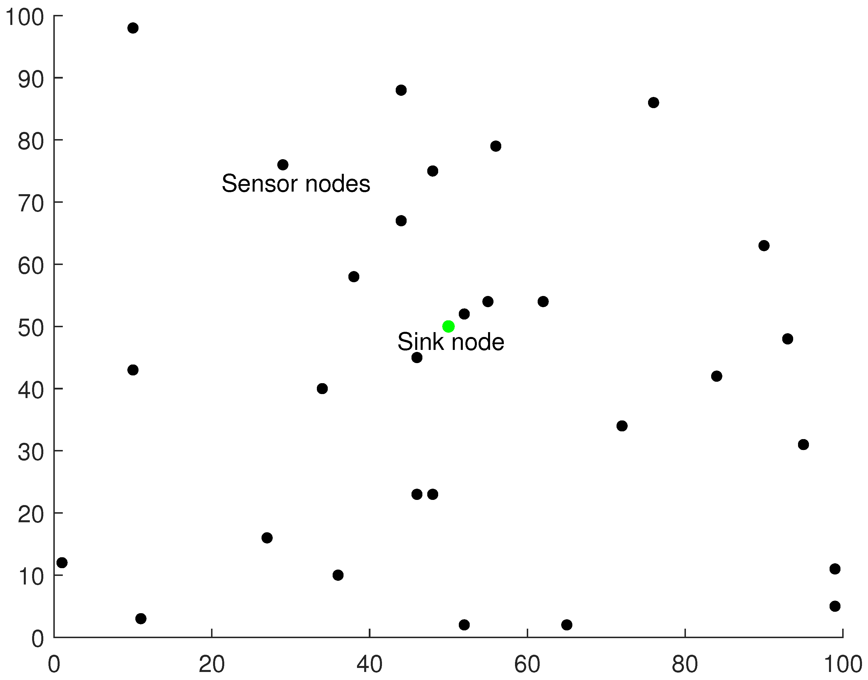
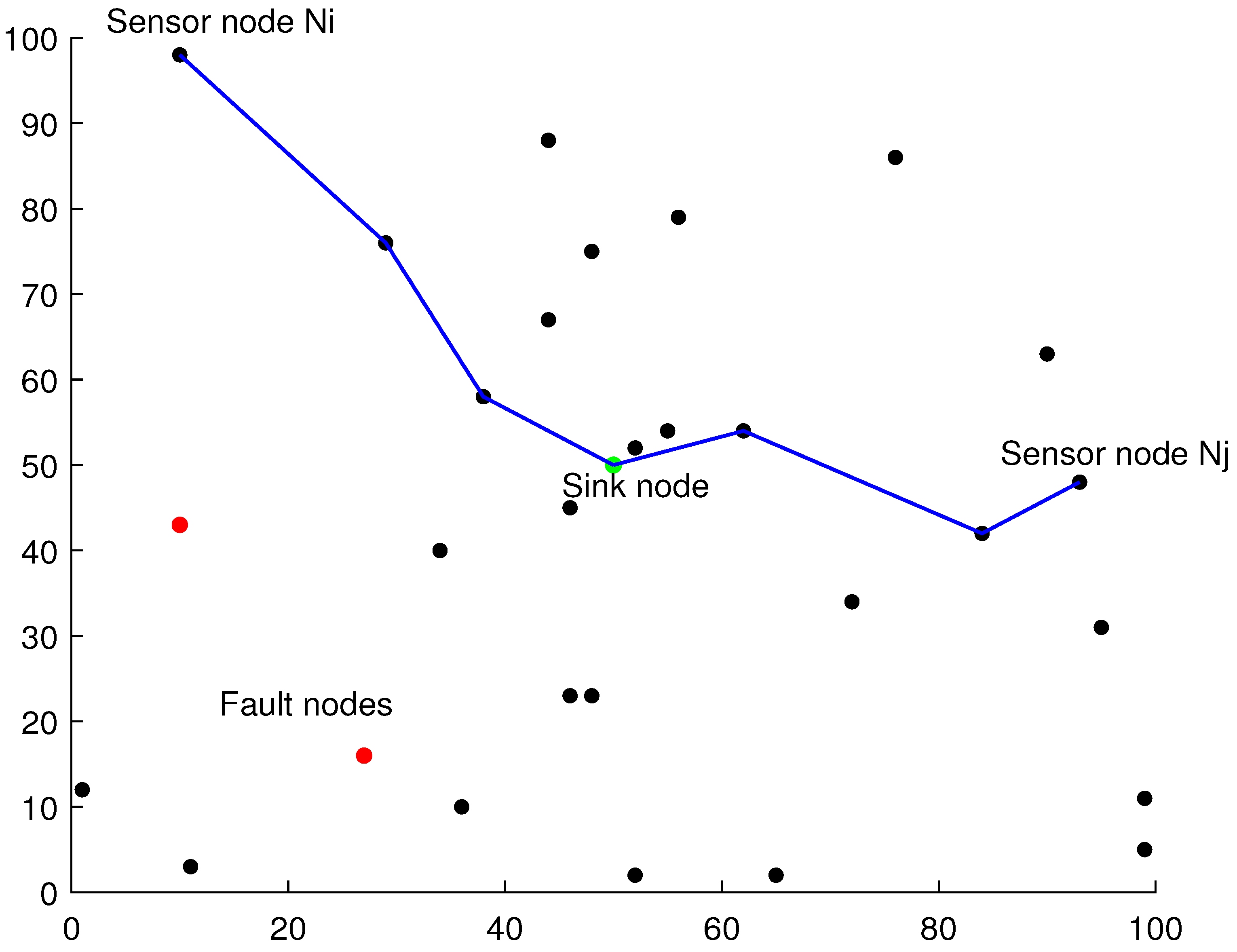
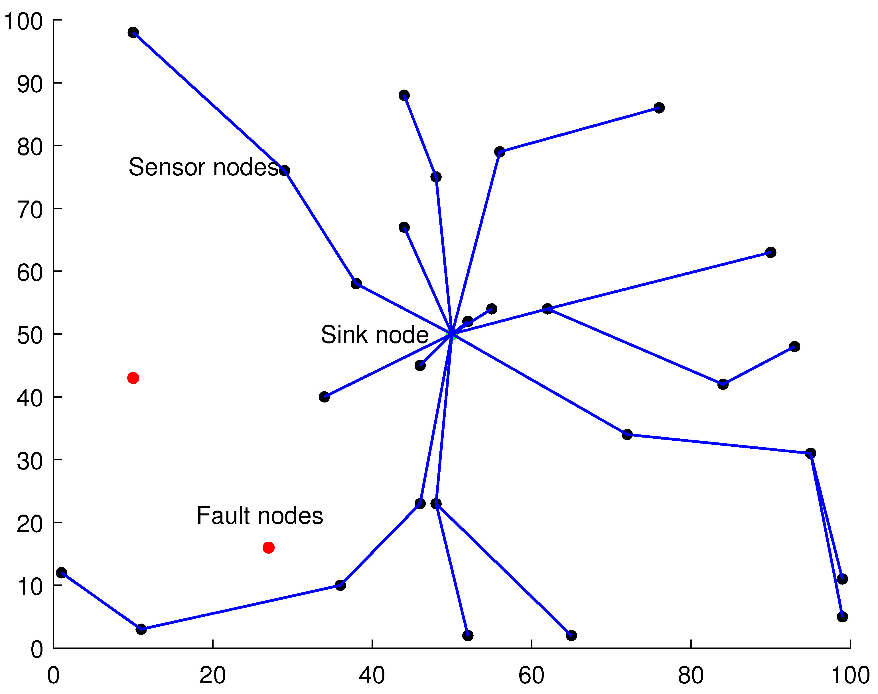
3.1. Network Model

We assume that in the multihop RPL wireless sensor network, n nodes form a set N that are fixed in a square region with side length L. Among them, $N_1$, located in the rectangular area’s center, is a sink node (i.e., gateway node or base station) with adequate computing resource and energy, which collects data from other nodes and is responsible for maintaining the network. The remaining $n-1$ resource-constrained sensor nodes denoted as $N_2$, $N_3$, …, $N_n$ are randomly scattered in this square region, as shown in Figure 1. During the initialization of the network, a sink node will assign a unique identifier to every sensor node, represented by a two-byte ID. All nodes have a fixed and limited transmission range $TL$.

In each collection cycle, the probability $P_{active}$ indicates that a sensor node is active, and the probability $P_{fault}$ means that a sensor node temporary fails. Whether individual sensor nodes are active or not is a mutually independent event, and an active sensor node sends packets as well as receives packets from others themselves. The failure of each sensor node is also independent of each other, and when a sensor node fails, it is unable to perform the activities of sending, forwarding, and receiving packets.

In this network model, point-to-point traffic (between devices inside the sensor network), point-to-multipoint traffic (from the sink node to a subset of sensor nodes), and multipoint-to-point traffic (from nodes inside the sensor network towards the sink node) are supported. Taking point-to-point traffic as an example, the shortest path from sensor node $N_i$ to sink node and then from sink node to sensor node $N_j$ without passing through the faulty node constitutes the routing path as shown in Figure 2. Where we assume that the upstream routing from sensor node $N_i$ to sink node and the downstream routing from sink node to sensor node $N_i$ are mirrored, i.e., the reverse path of the path from sensor node $N_i$ to sink node is the path from sink node to the sensor node $N_i$. As mentioned in several studies [26,27,28], it is assumed in RPL that the links are symmetric and that both directions of the links are connected. Then, the paths consisting of symmetric links have the reasonableness of symmetric assumption.

All routing paths in each collection cycle constitute the topology of the network as shown in Figure 3. It is assumed that the next hop sent by the sensor node to the sink node in the upstream routing is fixed, i.e., the path from any source node to the destination node in the cycle is unique if it exists.

3.2. Problem Statement

In the path recovery problem, a sequence consisting of the source node, the relay nodes, and the destination node for the successfully delivered packet k, denoted as $path(k)$, is supposed to be recovered. Since $path(k)$ goes through the sink node, it can be split into two subsequences, i.e., the upstream routing path $uppath(k)$, which comes from the source node to the sink node, and the downstream routing path $downpath(k)$, which is from the sink node to the destination node.

It is the upstream routing of all packets that ought to be recovered since it has been assumed that the upstream and downstream routing paths are mirrored and the active nodes in each collection cycle both send and receive packets. For example, as shown in Figure 4, in a certain collection cycle, while $path(k)$ denotes the path of packet k sent from node $N_i$ to node $N_j$ and $path(k^{\prime })$ denotes the path of packet $k^{\prime }$ sent from node $N_j$ to node $N_i$, those two paths just form a pair of inverse order. Then, when working on path recovery at the sink node, it is only necessary to recover the path $uppath(k)$ from node $N_i$ to sink node and the path $uppath(k^{\prime })$ from node $N_j$ to sink node, respectively, to obtain $path(k)$ and $path(k^{\prime })$. After that, $path(k)$ is the concatenated sequence of $uppath(k)$ and the reverse order of $uppath(k^{\prime })$.

Our goal is to correctly recover as many paths of all packets as possible for a continuous collection period. This goal, furthermore, can be translated into recovering the uplink routing path of the packets to the side of sink node as much as possible.

In each packet k, some information that will be recorded by the sink node and used in our path recovery algorithm is as follows:

• The source node $o(k)$ and destination node $d(k)$. These can be retrieved by the sink node based on the IPv6 address of the packet header, not requiring additional space overhead for the packet.
• The parent node $p(k)$ and grandparent node $g(k)$. The parent node $p(k)$ is the next hop of the source node, and the grandparent node $g(k)$ is the next hop of $p(k)$. To record the IDs of $p(k)$ and $g(k)$, an extra 4B of space is needed for a packet. The default values of $p(k)$ and $g(k)$ are empty. When the forwarder is the parent or grandparent node of the source node, its ID will be written into the corresponding field.
• The hash value of the upstream path of packet k is denoted as $h(k)$. It also refers to $hash(N_1,N_2,\dots ,Sink)$ where $(N_1,N_2,\dots ,Sink)$ represents a series of nodes ID. We set a hash function to identify an upstream path, which requires additional 2B space for a packet. Each node forwards packet k with a small computational overhead to update the $h(k)$, and the final $h(k)$ received by the sink node is the hash value that records an entire upstream path. The packets with the same hash value can be considered as going through the same path.
• The length of the uplink path, denoted as $len(k)$. This can be inferred from the Hop Limit of the IPv6 header without the additional space overhead of the packet.
• The timestamp $t(k)$. This can be inferred from the packet arrival time to which the packet belongs to the collection cycle, without the additional space overhead of the packet.

The performance of the path recovery algorithm can be measured by two metrics: $Accuracy$ and $GainLossRatio$:

• $Accuracy$. We define the $Accuracy$ of the path recovery problem as:

  $$Accuracy=\frac{Nu{m}_{correctRecovery}}{Nu{m}_{received}},$$

  (1)

  where $Nu{m}_{received}$ denotes the number of all successfully communicated packets, and $Nu{m}_{correctRecovery}$ denotes the number of all correctly recovered packets whose paths were correctly recovered. The purpose of path recovery is to improve the $Accuracy$ as much as possible.
• $GainLossRatio$. The meaning of this metric is how many bytes of gain we can exchange for one byte of overhead, which is defined as:

  $$GainLossRatio=\frac{Gain}{Loss},$$

  (2)

  where

  $$Gain=\sum _{i=1}^{Nu{m}_{received}}{C}_{ID}\times Le{n}_i\times R_i,$$

  (3)

  and

  $$Loss=Overhead\times Nu{m}_{generate}.$$

  (4)
  The $C_{ID}$ is the number of bytes occupied by a node ID, i.e., 2 bytes in our network model, and $Le{n}_i$ is the path length of the packet i. The $R_i\in \{0,1\}$ is an indicator variable of the packet i where $R_i=1$ means the packet path was correctly recovered, while $R_i=0$ means the packet path does not exist or has not been recovered correctly. The $Overhead$ is the extra overhead added to each packet for path recovery in this algorithm. As seen in the previous section, the overhead is 6 bytes in our network model, including 2 bytes for the parent node ID, 2 bytes for the grandparent node ID, and 2 bytes for the hash value. $Nu{m}_{generate}$ represents the packets generated by all active nodes, although some source nodes could not be successfully communicated to the destination node due to a failure of the original route node, which is limited by the transmission distance.

4. Design of LiPa

4.1. Solution Overview

Our proposed algorithm consists of two parts, i.e., path information encoding during packet delivery and path recovery of the received information at the server-side.

During packet delivery, the information required for path recovery is passed along the uplink path from the source node to the sink node. The information needed in packet k is as follows: the source node $o(k)$ and the destination node $d(k)$, which can be looked up by the sink node based on the IP address in the IPv6 header; the length of the uplink path $len(k)$; the timestamp $t(k)$, which can be directly inferred from the IPv6 header; and three additional data—the parent node $p(k)$ and grandparent node $g(k)$ combined with the hash of the uplink path $h(k)$.

For the parent node, $p(k)$, it will take 2 bytes of the packet space to store the ID of the parent node. We specify that when a forwarder finds $p(k)$ empty in a packet, the forwarder is the parent node and will write its ID into $p(k)$. For the grandparent node $g(k)$, the space of 2 bytes of the packet is occupied to store the ID of the grandparent node. Analogously, when $p(k)$ is not empty and $g(k)$ is empty, the forwarder is the grandparent node and needs to write its ID to $g(k)$. Note that once $p(k)$ or $g(k)$ are filled in, their value will not be changed. In addition, if the parent node or grandparent node is already a sink node, the corresponding value will be all zeros. For the upstream path $h(k)$, 2 bytes of overhead is used to store the hash value of the route, which is continuously updated during the transmission. Starting from the source node, for each node of such an upstream route, they update the hash value by the following functions [12]:

$$h_i(k)=h_{i-1}(k)\oplus f_{ID}(i)$$

(5)

based on their ID value, where

$$f_{ID}(i)=(ID\times \alpha <<\lceil lo{g}_{2}ID\rceil )mod{2}^m,$$

(6)

$$h_1(k)=f_{ID}(1).$$

(7)

We set $m=16$, i.e., the number of bits occupied by this hash is 16, and the space size is 2 bytes. Note that LiPa is used to extract the full path information by measurements of the packet traces. It works independently from the routing protocols. The 6 bytes overhead, i.e., the $p(k)$, $g(k)$, and $h(k)$ fields, are directly appended to the packet to participate in the transmission, rather than an additional packet being routed through to recover the path.

For server-side information processing, the above packet information is used for uplink path recovery within the sliding observation window to recover the point-to-point routing path through the mirroring feature. Specifically, the required information mentioned above is recorded when the packet arrives at the sink node through the uplink; then, the packet is forwarded following the downlink to the destination node. We set a sliding window of the following size:

$$\tau =\left[\frac{1}{Rati{o}_{active}}\right],$$

(8)

where $Rati{o}_{active}$ is the proportion of active nodes in the network. At time t, the sink node will recover all packets’ paths in the period $[t-\tau ,t]$. For path recovery within this sliding window, the possible correlations in different paths are explored, starting from the short one-hop and two-hop paths based on the information of the parent and grandparent nodes and then iteratively solving for more unknown paths. To ensure whether the recovered paths are correct, the hash value of the uplink is needed.

During the running of system, the operation of LiPa is divided into two operation parts. (1) For sensor nodes, the information encoded during packet delivery is updated by every forwarder, and their IDs are attached to headers when they work as the first-hop or second-hop forwarder of a packet. (2) For the sink node which collects packets from all sensor nodes, the received packet information can be merged to perform the recovery algorithm in the style of online (real-time) or offline.

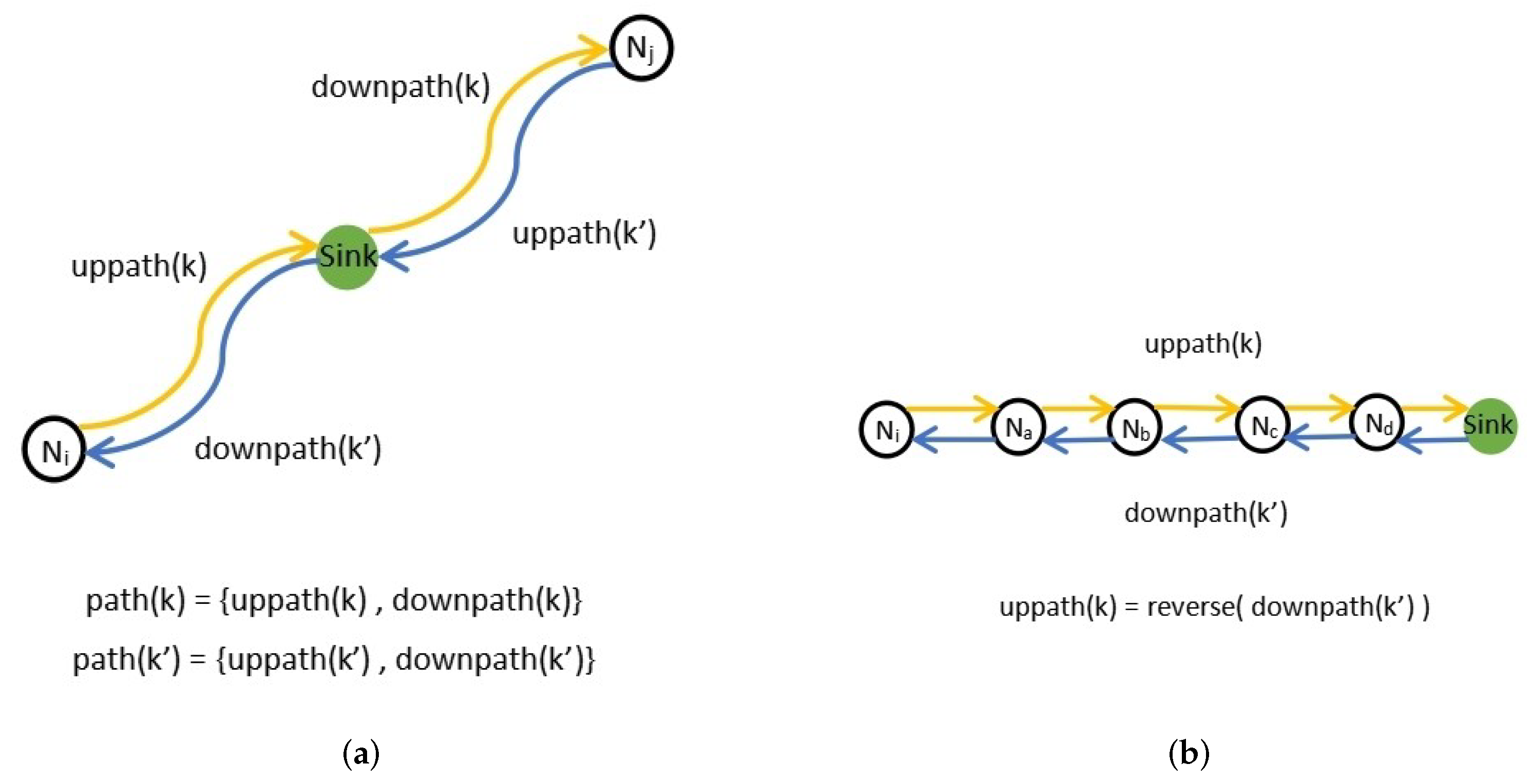
4.2. Path Correlation Inference

The core operation of path recovery lies in the correlation inference of paths. The question we want to answer is whether two paths are correlated? What kind of correlations exists? How can we use such a correlation to recover an unknown path?

Algorithm 1 answers these questions above. For a packet i whose path is unknown and a packet k whose path is known already, the algorithm examines whether a correlation exists between the two paths. If it does, it uses the $path(k)$ of packet k to recover the $path(i)$ of packet i. The different correlations and the corresponding methods of path recovery are summarized in the following cases.

The following examples will describe different correlation and path recovery methods.

Case 1: When $len(i)$ of packet i is two hops longer than $len(k)$ of packet k, the sink will check whether the grandpa node $g(i)$ of packet i is the source node $o(k)$ of packet k. If it is, $path(i)$ is the combination of $o(i)$, $p(i)$, and $path(k)$. To avoid the error of $path(k)$ making the $path(i)$ is also recovered incorrectly, it is necessary to evaluate whether the hash value $h(i)$ is equal to $hash(o(i),p(i),path(k))$. This recovery path can be assigned to $path(i)$ if equal. The example is given in Figure 5a: In a collection cycle, node K generates packet $K1$, and node A generates packet $A1$. Since K is the grandpa node of A, $path(K1)$ with path $(K,G,H,I)$ can be used to recover $path(A1)$, i.e., $path(A1)=(A,B,K,G,H,I)$.

Case 2: When $len(i)$ is one hop longer than $len(k)$, the sink will determine whether $p(i)$ is equal to $o(k)$. If so, $path(i)$ is the combination of $o(i)$ and $path(k)$. Similarly, once $h(i)$ is equal to $hash(o(i),path(k))$, this recovery path can be assigned to $path(i)$. The example is given in Figure 5b: In a collection cycle, node K generates packet $K1$, and node B generates packet $B2$. Since K is the parent node of B, $path(K1)$ with path $(K,G,H,I)$ can be used to recover $path(B2)$, i.e., $path(B2)=(B,K,G,H,I)$.

Algorithm 1 The Recovery Core Algorithm.

Require:k: a packet whose path has been recovered;      i: a packet whose path is unknown; Output:True or False: whether packet k can be used to recover the path of packet i; 1: if$len(i)-len(k)\notin \{2,1,0,-1\}$then 2:       return $False$ 3: end if 4: if$len(i)-len(k)\equiv 2$then 5:       if $g(i)\equiv o(k)\mathbf{and}h(i)\equiv hash(o(i),p(i),path(k))$ then 6:             $path(i)\leftarrow (o(i),p(i),path(k))$        $//Case1$ 7:             return $True$ 8:       end if 9: else 10:       if $len(i)-len(k)\equiv 1$ then 11:             if $p(i)\equiv o(k)\mathbf{and}h(i)\equiv hash(o(i),path(k))$ then 12:                    $path(i)\leftarrow (o(i),path(k))$  $//Case2$ 13:                    return $True$ 14:             else 15:                    if $g(i)\equiv p(k)\mathbf{and}h(i)\equiv hash(o(i),p(i),path(k)-o(k))$ then 16:                          $path(i)\leftarrow (o(i),p(i),path(k)-o(k))$  $//Case3$ 17:                          return $True$ 18:                    end if 19:             end if 20:       else 21:             if $len(i)-len(k)\equiv 0$ then 22:                    if $p(i)\equiv p(k)\mathbf{and}h(i)\equiv hash(o(i),path(k)-o(k))$ then 23:                          $path(i)\leftarrow (o(i),path(k)-o(k))$  $//Case4$ 24:                          return $True$ 25:                    else 26:                          if $g(i)\equiv g(k)\mathbf{and}h(i)\equiv hash(o(i),p(i),path(k)-o(k)-p(k))$ then 27:                              $path(i)\leftarrow (o(i),p(i),path(k)-o(k)-p(k))$  $//Case5$ 28:                              return $True$ 29:                          end if 30:                    end if 31:             else  $//len(i)-len(k)\equiv -1$ 32:                    if $p(i)\equiv g(k)\mathbf{and}h(i)\equiv hash(o(i),path(k)-o(k)-p(k))$ then 33:                          $path(i)\leftarrow (o(i),path(k)-o(k)-p(k))$  $//Case6$ 34:                          return $True$ 35:                    end if 36:             end if 37:       end if 38: end if 39: return$False$

Case 3: When $len(i)$ is one hop longer than $len(k)$, there is another possibility that $g(i)$ is equal to $p(k)$. In this case, $path(i)$ is the combination of $o(i)$, $p(i)$, and the part of $path(k)$ that removes $o(k)$. If $h(i)$ is equal to $hash(o(i),p(i),path(k)-o(k))$, this recovery path can be assigned to $path(i)$. An example is given in Figure 5c: In a collection cycle, node K generates packet $K1$, and node C generates packet $C3$. Since the grandparent node of C and the parent node of K are both G, $path(K1)$ with path $(K,G,H,I)$ can be used to recover $path(C3)$, i.e., $path(C3)=(C,D,G,H,I)$.

Case 4: When $len(i)$ is equal to $len(k)$ and $p(i)$ is equal to $p(k)$, $path(i)$ is the combination of $o(i)$ and the part of $path(k)$ that removes $o(k)$. If $h(i)$ is equal to $hash(o(i),path(k)-o(k))$, this recovery path can be assigned to $path(i)$. The example is given in Figure 5d: In a collection cycle, node K generates packet $K1$, and node D generates packet $D4$. Since the parent node of D and the parent node of K are both G, $path(K1)$ with path $(K,G,H,I)$ can be used to recover $path(X4)$, i.e., $path(D4)=(D,G,H,I)$.

Case 5: When $len(i)$ is equal to $len(k)$, another possibility is that $g(i)$ and $g(k)$ are the same. In this case, $path(i)$ is the combination of $o(i)$, $p(i)$, and the part of $path(k)$ that removes $o(k)$ and $p(k)$. Similarly, this recovery path can be assigned to $path(i)$ if $h(i)$ is equal to $hash(o(i),p(i),path(k)-o(k)-p(k))$. The example is given in Figure 5e: In a collection cycle, node K generates packet $K1$, and node E generates packet $E5$. Since the grandpa node of E and the grandpa node of K are both H, $path(K1)$ with path $(K,G,H,I)$ can be used to recover $path(E5)$, i.e., $path(E5)=(E,F,H,I)$.

Case 6: When $len(i)$ is one hop less than $len(k)$, $path(i)$ is the combination of $o(i)$ and the part of $path(k)$ that removes $o(k)$ and $p(k)$ if $p(i)$ is equal to $g(k)$. Then, this recovery path can be assigned to $path(i)$ after determining that $h(i)$ is $hash(o(i),path(k)-o(k)-p(k))$. An example is given in Figure 5f: In a collection cycle, node K generates packet $K1$, and node F generates packet $F6$. Since the parent node of F and the grandparent node of K are both H, $path(K1)$ with path $(K,G,H,I)$ can be used to recover $path(F6)$, i.e., $path(F6)=(F,H,I)$.

4.3. Iterative Path Recovery

The proposed LiPa will iteratively use the known paths to recover unknown paths until no more paths can be recovered.

Algorithm 2 gives the complete flow of this algorithm. At moment t, the sliding window $[t-\tau ,t]$ is used as the observation interval. The input is two sets, $Pinit$ and $Punknown$. Since the packets record the parent and grandpa nodes, $Pinit$ is formed by packets whose path length is one or two hops, while the rest of the packets have unknown form $Punknown$. The packets with unknown paths will try to recover unknown paths according to the path correlation inference given in Algorithm 1. The algorithm terminates when no more unknown paths or no more paths can be recovered. The output is the packets with recovered paths.

Algorithm 2 The Lightweight Path Recovery Algorithm.

Require:$P_{init}$: a set of packets during $[t-\tau ,t]$ whose paths have been recovered;      $P_{unknown}$: a set of packets during $[t-\tau ,t]$ whose paths are unknown; Output: $P_{known}$: a set of packets during $[t-\tau ,t]$ whose paths are recovered; 1: $P_{known}\leftarrow P_{init}$ 2: while$P_{unknown}\ne \left\{\right\}$do 3:      $P_{learn}\leftarrow P_{known}$ 4:      for each packet $k\in P_{known}$ do 5:             for each packet $i\in P_{unknown}$ do 6:                   if $RecoveryCore(k,i)\equiv TRUE$ then       // Recalling the Algorithm 1 7:                         $P_{learn}\leftarrow P_{learn}\cup i$ 8:                         $P_{unknown}\leftarrow P_{unknown}-i$ 9:                   end if 10:             end for 11:      end for 12:      if $P_{learn}\equiv P_{known}$ then 13:             Break 14:      end if 15:      $P_{known}\leftarrow P_{learn}$ 16: end while

Time complexity analysis. We set the number of nodes to be N, the $Rati{o}_{active}$ to be $\alpha$, $\alpha \in [0,1]$, and the window size to be $\tau$. For Algorithm 1 (i.e., The Recovery Core Algorithm), its complexity is $O(Alg.1)=O(1)$, due to it consisting of up to seven operations of if-then-else-then. For Algorithm 2 (i.e., The Lightweight Path Recovery Algorithm), the basic operation is to call Algorithm 1. As all active nodes will send packets, and the number of packets at each time slot is $\alpha \times N$. The window size $\tau =\left[\frac{1}{\alpha }\right]$ for path recovery is obtained from Equation (8), so the total number of packets in the time interval $[t-\tau ,t+\tau ]$ is N, which consists of $Pinit$ and $Punknown$. The algorithm’s complexity for Lines 4–11 in Algorithm 2 is obtained as $O(N^2)$. Since packet k with $len(k)$ is able to recover packet i with $len(i)\in [len(k)-1,len(k)+2]$ and the algorithm terminates when no more path can be recovered, the executed times of the whole loop can be considered as N. Therefore, the total complexity of the LiPa algorithm is $O(N^3)$.

The characteristic of this algorithm is that, for an unknown path of packet k at time t, all known paths in the time interval $[t-\tau ,t+\tau ]$ will try to recover using correlation, which makes the search space of the problem expand. The setting of $\tau$, as given in Equation (8), keeps the computational effort at a suitable level.

5. Performance Evaluation and Analysis

Based on a series of simulations, this section compares the performance of LiPa with two state-of-the-art approaches, iPath [12] and CSPR [13], to analyze the effectiveness and efficiency of our proposal in different network environments.

5.1. Evaluation Setup

Our simulation experiments are performed on Matlab, conducted in a 1000 × 1000 m² field. The sink node is located in the center of this field, and the sensor nodes are randomly distributed. The maximum transmission range of each node is 100 m. The number of nodes varies from 100 to 500, the active ratio of nodes (i.e., the percentage of nodes generating packets) varies from 10% to 100%, and the percentage of fault nodes is set to 2.5%, 5%, 7.5%, or 10%.

The Accuracy is defined as $\frac{Nu{m}_{correctRecovery}}{Nu{m}_{received}}\times 100\%$, reflecting the effectiveness of the path recovery algorithm. The Gain–Loss Ratio is defined as $\frac{Gain}{Lost}\times 100\%$, which reflects the tradeoff between the overhead and the benefit of the path recovery algorithm.

We compare LiPa with the iPath and CSPR algorithms. iPath utilizes the information of the parent node carried by packets and the hash value identifying the path in a collection cycle, recovering the routing path by correlating the paths between different packets. CSPR employs a compression sensing technique, allowing each packet to carry partially encoded information, then collects and decodes information of path recovery in the multi-collection cycles to obtain the routing paths.

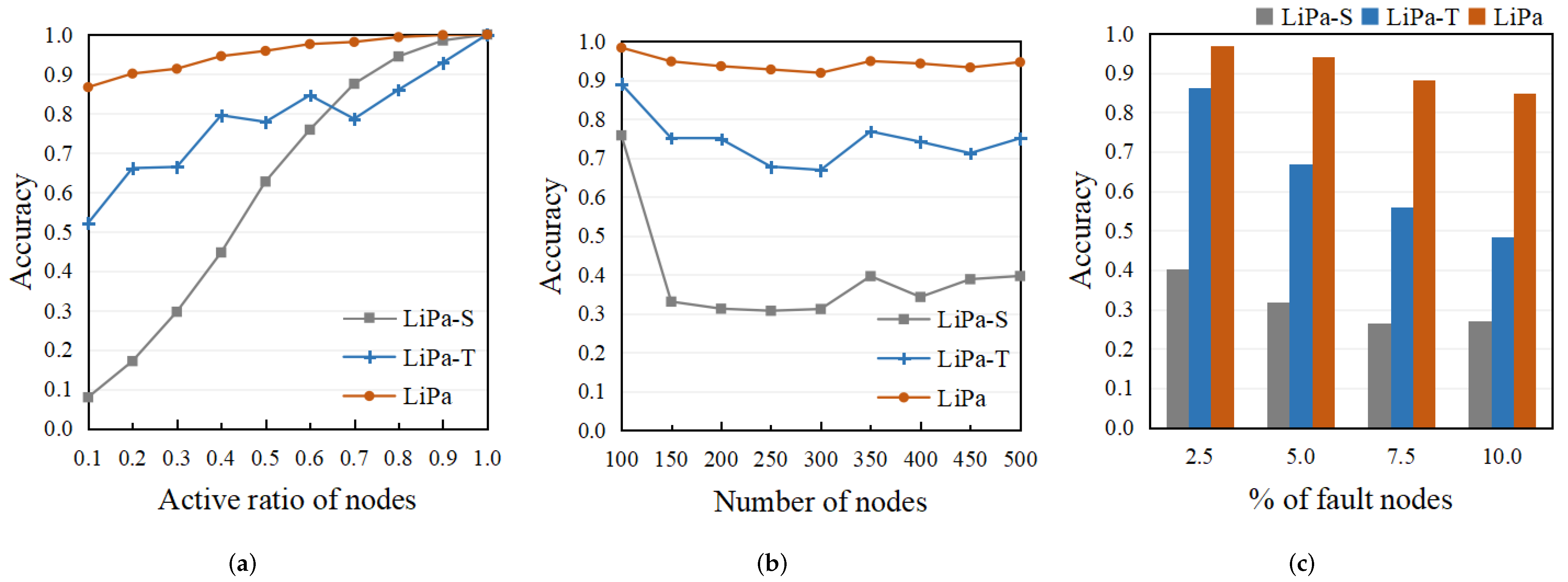
5.2. Performance Improvement Analysis

Our proposed LiPa algorithm has two features compared to other existing works: On the one hand, it adds the information of grandparent nodes in addition to that of parent nodes. On the other hand, it utilizes the information of multiple collection cycles instead of the present cycle only. Therefore, we specifically analyze the effect of these two features on the performance improvement of the LiPa algorithm separately. To this end, two variation of LiPa are introduced:

LiPa-S mainly leverages the spatial information of the parent and grandparent nodes but sets $\tau =0$, i.e., the LiPa algorithm with a sliding window size of 1. Without the temporal information of multiple collection cycles, this variation is introduced to verify the effectiveness of the adaptive sliding window of LiPa.

LiPa-T mainly uses the temporal information of the sliding window size of $\tau =\left[\frac{1}{Rati{o}_{active}}\right]$ but only records the information of the parent node, i.e., the LiPa algorithm with only two path relevance cases, case 2 and case 4, mentioned in Section 4. Without sufficient spatial information, we can observe the performance improvement of LiPa by appending the grandpa node’s information, thus adding the other four possible path correlations cases mentioned in Section 4.

Figure 6 shows the accuracy of LiPa-S, LiPa-T, and LiPa in different network scenarios. As shown in Figure 6a, when the number of nodes is 300, and the percentage of fault nodes is 5%, the accuracy of the 3 LiPa algorithms improves as the active ratio of nodes changes, and LiPa’s accuracy is consistently higher than LiPa-S and LiPa-T. The accuracy improvement of the LiPa algorithm over LiPa-S is 33% on average and up to 78%. The accuracy improvement of the LiPa algorithm over LiPa-T reaches an average of 19% and 34% at the most. As shown in Figure 6b, when the percentage of fault nodes is 5%, and the active ratio of nodes is 30%, the accuracy of the 3 LiPa algorithms decreases as the number of nodes changes, but the accuracy of LiPa is still consistently higher than that of LiPa-S and LiPa-T. The accuracy improvement of the LiPa algorithm over LiPa-S reaches an average of 55% and a maximum of 62%. The accuracy improvement of the LiPa algorithm over LiPa-T reaches an average of 19% and 25% at most. As shown in Figure 6c, when the number of nodes is 300, and the active ratio of nodes is 30%, the accuracy of the 3 LiPa algorithms decreases as the percentage of fault nodes changes, but the accuracy of LiPa is still consistently higher than that of LiPa-S and LiPa-T. The accuracy improvement of the LiPa algorithm over LiPa-S is 59% on average. The accuracy improvement of the LiPa algorithm over LiPa-T is the highest, reaching an average of 26%. These results are because both LiPa-S and LiPa-T are neutered versions of LiPa, drawing only one of the two features of LiPa.

We can conclude that: (1) From the difference between LiPa and LiPa-S, our practice of setting an observation window can improve the performance by about 50% on average. (2) From the gap between LiPa and LiPa-T, our practice of appending grandparent nodes can improve the performance by about 20% on average. (3) In combination, the performance improvement from setting observation windows is more significant than appending grandparent nodes.

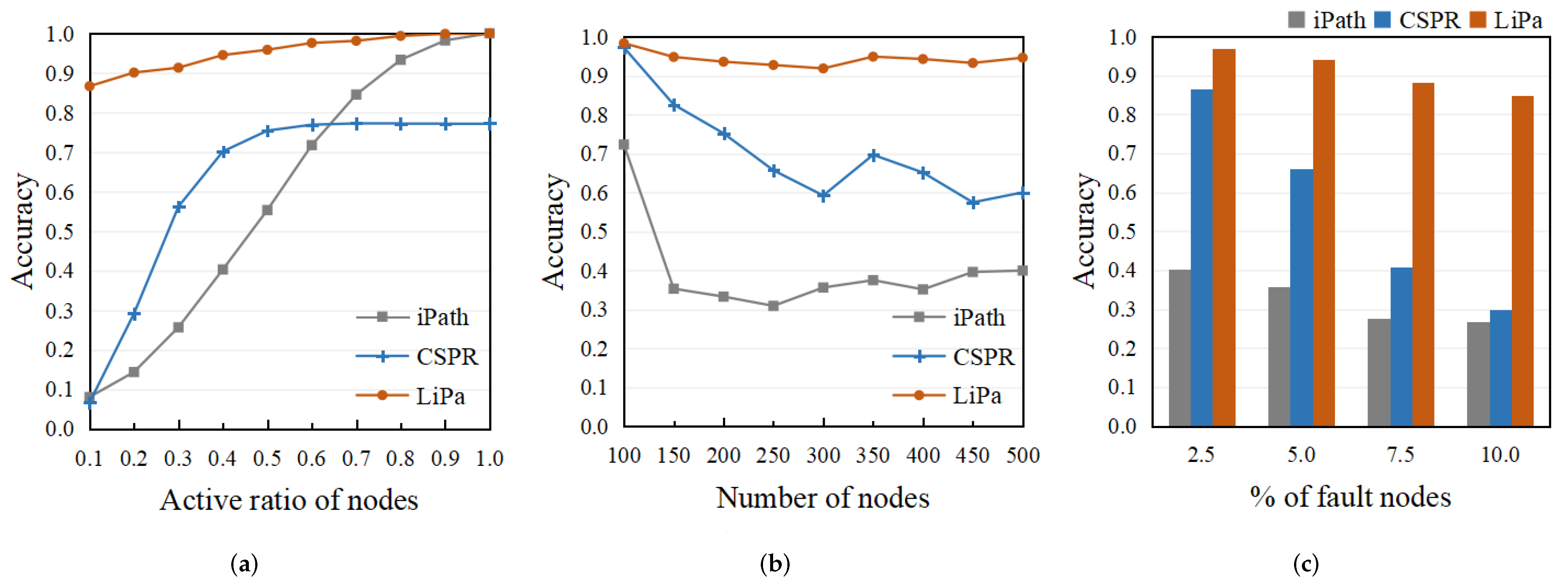
5.3. Comparison of the Accuracy

Figure 7 demonstrates the accuracy of the three algorithms in different network scenarios. As shown in Figure 7a, when the number of nodes is 300, and the percentage of fault nodes is 5%, the accuracy of the 3 algorithms improves as the active ratio of the nodes changes. This is because, with the active ratio of the nodes increasing, the more packet information the algorithm can utilize, the more beneficial it is to path recovery. The accuracy of the LiPa algorithm is consistently higher than iPath and CSPR, improving by over 30% on average. As shown in Figure 7b, when the percentage of fault nodes is 5% and the active ratio of the nodes is 30%, the accuracy of LiPa and CSPR is stable, while iPath decreases as the number of nodes changes. This is because the higher the number of nodes, the more complex the network topology is. iPath has a specific performance bottleneck by using only the path correlations at that moment. In contrast, LiPa and iPath can use the information for longer time durations to solve the complex topology. The accuracy of LiPa is still consistently higher than that of the other 2 algorithms, improving by over 50% on average compared with iPath and over 20% on average compared with CSPR. As shown in Figure 7c, when the number of nodes is 300, and the active ratio of nodes is 30%, the accuracy of the 3 algorithms decreases as the percentage of fault nodes changes. This is because the more fault nodes there are, the more dynamic the network topology is and the more difficult it is to recover the path. The accuracy of LiPa is still consistently higher than that of iPath and CSPR, improving by over 55% on average compared with iPath and by over 35% on average compared with CSPR.

We can conclude that LiPa consistently outperforms iPath and CSPR in the above network scenarios. The reason for this is that LiPa takes similar features of both iPath and CSPR and makes further enhancements. On the one hand, both LiPa and iPath have the idea of path correlation. Still, LiPa uses the information of parent and grandparent nodes to extend the possible cases of correlation, using the information of a sliding window to perform path recovery. On the other hand, both LiPa and CSPR utilize temporal information, but LiPa processes this information by path correlations rather than compression-aware methods.

5.4. Comparison of the Gain–Loss Ratio

Figure 8 compares the gain–loss ratio of the three algorithms in different network scenarios. The gain–loss ratio is a composite performance metric that reflects the ratio of the gain (i.e., the numerical metric of correctly recovered paths) to the overhead (i.e., the sum of the additional storage overhead used for recovery), which is defined in Equations (2)–(4). In other words, this measurement covers not only the accuracy but also the length of the recovered path and overhead. A larger gain–loss ratio for an algorithm means that it has a higher accuracy or a smaller overhead, or both.

As shown in Figure 8a, when the number of nodes is 300, and the percentage of fault nodes is 5%, the gain–loss ratio of the 3 algorithms improves as the active ratio of nodes changes. The overhead of the three algorithms is constant individually, so their accuracy determines the trend of their respective gain–loss ratios. The gain–loss ratio of LiPa grows in a high range because its accuracy rate also grows in an increased range. CSPR’s gain–loss ratio grows to a certain point and remains stable because CSPR’s accuracy has stabilized when the node activity rate is more significant than 50%. Furthermore, the accuracy of the LiPa algorithm is consistently higher than iPath and CSPR. The difference among their gain–loss ratios is affected by both accuracy and overhead. Among them, LiPa and iPath have smaller overheads, requiring only 6 bits of extra overhead per packet. However, CSPR, with low accuracy, has an extra overhead of 8 bits per packet, which makes its gain–loss ratio much lower than the other two algorithms. As shown in Figure 8b, when the percentage of fault nodes is 5%, and the active ratio of nodes is 30%, the gain–loss ratios of the 3 algorithms start fluctuating after improving to a certain level. Their respective accuracy rates influence this. Meanwhile, the gain–loss ratio of LiPa is still consistently higher than that of the other two algorithms. Among them, LiPa’s higher gain–loss ratio than iPath is due to its higher accuracy rate, and LiPa’s higher gain–loss ratio than CSPR is due to the former’s higher accuracy rate and its more negligible overhead. As shown in Figure 8c, when the number of nodes is 300, and the active ratio of nodes is 30%, LiPa and iPath are more stable, while CSPR has a specific downward trend, which is also influenced by their individual accuracy rates. Moreover, the gain–loss ratio of LiPa is still consistently higher than that of iPath and CSPR. For similar reasons, in this network scenario, LiPa has higher accuracy than iPath and CSPR while having a lower additional overhead than CSPR.

We can conclude that: LiPa’s gain–loss ratio consistently outperforms iPath and CSPR in the above network scenarios. This is because, on the one hand, LiPa’s higher accuracy rate leads to more significant gains; on the other hand, LiPa’s overhead is not larger than CSPR and iPath. Thus, the higher gain ratio of LiPa is reflected.

6. Conclusions

In this paper, we propose a lightweight path recovery algorithm in a dynamic network, namely, LiPa. Based on the path correlation inference in the network topology, LiPa reconstructs the routing path of each packet within a sliding window that varies according to the activity the ratio of nodes. The distinctive feature of LiPa is that the path recovery is performed in two dimensions: temporal information and spatial information. We analyze the performance improvement effect of both dimensions of LiPa and compare it with two related approaches. The experimental results show that LiPa exhibits superior performance in different network settings.

For the limitations, the system model denotes the target scenario of our work is a wireless sensor network (WSN) with fixed-location nodes. The proposed LiPa cannot be appropriately applied in mobile networks (e.g., vehicular networks, UAV networks) whose path correlations are weak and frequently change due to the movement of nodes.

In future work, an asymmetric network with RPL routing should be further exploited. The uplink and downlink routing is assumed to be symmetric in our present work. However, when this assumption is not satisfied, both the uplink and downlink paths should be reconstructed for point-to-point path recovery.

References

1. Winter, T.; Thubert, P.; Brandt, A.; Hui, J.W.; Kelsey, R.; Levis, P.; Pister, K.; Struik, R.; Vasseur, J.P.; Alexander, R.K.; et al. RPL: IPv6 Routing Protocol for Low-Power and Lossy Networks. RFC 2012, 6550, 1–157. [Google Scholar]
2. Glissa, G.; Rachedi, A.; Meddeb, A. A Secure Routing Protocol Based on RPL for Internet of Things. In Proceedings of the 2016 IEEE Global Communications Conference (GLOBECOM), Washington, DC, USA, 4–8 December 2016; pp. 1–7. [Google Scholar] [CrossRef]
3. Hashemi, S.Y.; Shams Aliee, F. Dynamic and comprehensive trust model for IoT and its integration into RPL. J. Supercomput. 2019, 75, 3555–3584. [Google Scholar] [CrossRef]
4. Hariharakrishnan, J.; Natarajan, B. Adaptability Analysis of 6LoWPAN and RPL for Healthcare applications of Internet-of-Things. J. ISMAC 2021, 2, 69–81. [Google Scholar] [CrossRef]
5. Caldeira, J.M.; Rodrigues, J.J.; Lorenz, P. Toward ubiquitous mobility solutions for body sensor networks on healthcare. IEEE Commun. Mag. 2012, 50, 108–115. [Google Scholar] [CrossRef]
6. Abdel Hakeem, S.A.; Hady, A.A.; Kim, H. RPL Routing Protocol Performance in Smart Grid Applications Based Wireless Sensors: Experimental and Simulated Analysis. Electronics 2019, 8, 186. [Google Scholar] [CrossRef] [Green Version]
7. Wang, D.; Tao, Z.; Zhang, J.; Abouzeid, A.A. RPL based routing for advanced metering infrastructure in smart grid. In Proceedings of the 2010 IEEE International Conference on Communications Workshops, Capetown, South Africa, 23–27 May 2010; pp. 1–6. [Google Scholar]
8. Istomin, T.; Kiraly, C.; Picco, G.P. Is RPL Ready for Actuation? A Comparative Evaluation in a Smart City Scenario. In Wireless Sensor Networks; Abdelzaher, T., Pereira, N., Tovar, E., Eds.; Springer International Publishing: Cham, Switzerland, 2015; pp. 291–299. [Google Scholar]
9. Handigol, N.; Heller, B.; Jeyakumar, V.; Mazières, D.; McKeown, N. I Know What Your Packet Did Last Hop: Using Packet Histories to Troubleshoot Networks. In Proceedings of the 11th USENIX Conference on Networked Systems Design and Implementation (NSDI’14), Seattle, WA, USA, 2–4 April 2014; USENIX Association: Berkeley, CA, USA, 2014; pp. 71–85. [Google Scholar]
10. Malekzadeh, A.; MacGregor, M.H. Network topology inference from end-to-end unicast measurements. In Proceedings of the 2013 27th International Conference on Advanced Information Networking and Applications Workshops, Barcelona, Spain, 25–28 March 2013; pp. 1101–1106. [Google Scholar]
11. Larmore, G.; Harrison, W.K. Active Topology Inference in Store, Code, and Forward Networks. In Proceedings of the 2018 15th International Symposium on Wireless Communication Systems (ISWCS), Lisbon, Portugal, 28–31 August 2018; pp. 1–6. [Google Scholar] [CrossRef]
12. Gao, Y.; Dong, W.; Chen, C.; Bu, J.; Wu, W.; Liu, X. iPath: Path Inference in Wireless Sensor Networks. IEEE/ACM Trans. Netw. 2016, 24, 517–528. [Google Scholar] [CrossRef]
13. Liu, Z.; Li, Z.; Li, M.; Xing, W.; Lu, D. Path Reconstruction in Dynamic Wireless Sensor Networks Using Compressive Sensing. IEEE/ACM Trans. Netw. 2016, 24, 1948–1960. [Google Scholar] [CrossRef] [Green Version]
14. Lu, X.; Dong, D.; Liao, X.; Li, S.; Liu, X. PathZip: A lightweight scheme for tracing packet path in wireless sensor networks. Comput. Netw. 2014, 73, 1–14. [Google Scholar] [CrossRef]
15. Liu, Y.; Liu, K.; Li, M. Passive Diagnosis for Wireless Sensor Networks. IEEE/ACM Trans. Netw. 2010, 18, 1132–1144. [Google Scholar] [CrossRef] [Green Version]
16. Keller, M.; Beutel, J.; Thiele, L. How Was Your Journey? Uncovering Routing Dynamics in Deployed Sensor Networks with Multi-Hop Network Tomography. In Proceedings of the 10th ACM Conference on Embedded Network Sensor Systems (SenSys’12), Toronto, ON, Canada, 6–9 November 2012; Association for Computing Machinery: New York, NY, USA, 2012; pp. 15–28. [Google Scholar] [CrossRef]
17. Dong, W.; Gao, Y.; Cao, C.; Zhang, X.; Wu, W. Universal Path Tracing for Large-Scale Sensor Networks. IEEE/ACM Trans. Netw. 2020, 28, 447–460. [Google Scholar] [CrossRef]
18. Zhu, X.; Lu, Y.; Zhang, J.; Wei, Z. Routing Topology Inference for Wireless Sensor Networks Based on Packet Tracing and Local Probing. IEICE Trans. Commun. 2019, E102.B, 122–136. [Google Scholar] [CrossRef]
19. Dong, W.; Cao, C.; Zhang, X.; Gao, Y. Understanding path reconstruction algorithms in multihop wireless networks. IEEE/ACM Trans. Netw. 2018, 27, 1–14. [Google Scholar] [CrossRef]
20. Kim, H.S.; Ko, J.; Culler, D.E.; Paek, J. Challenging the IPv6 Routing Protocol for Low-Power and Lossy Networks (RPL): A Survey. IEEE Commun. Surv. Tutor. 2017, 19, 2502–2525. [Google Scholar] [CrossRef]
21. Livadariu, I.; Elmokashfi, A.; Dhamdhere, A. Characterizing IPv6 control and data plane stability. In Proceedings of the IEEE INFOCOM 2016—The 35th Annual IEEE International Conference on Computer Communications, San Francisco, CA, USA, 10–14 April 2016; pp. 1–9. [Google Scholar] [CrossRef]
22. Lai, G.S. Detection of wormhole attacks on IPv6 mobility-based wireless sensor network. EURASIP J. Wirel. Commun. Netw. 2016, 2016, 274. [Google Scholar] [CrossRef]
23. Waddington, D.G.; Chang, F.; Viswanathan, R.; Yao, B. Topology Discovery for Public IPv6 Networks. SIGCOMM Comput. Commun. Rev. 2003, 33, 59–68. [Google Scholar] [CrossRef]
24. Gao, Y.; Dong, W.; Chen, C.; Bu, J.; Liu, X. Towards reconstructing routing paths in large scale sensor networks. IEEE Trans. Comput. 2015, 65, 281–293. [Google Scholar] [CrossRef]
25. Liu, R.; Liang, Y.; Zhong, X. Monitoring routing topology in dynamic wireless sensor network systems. In Proceedings of the 2015 IEEE 23rd International Conference on Network Protocols (ICNP), San Francisco, CA, USA, 10–13 November 2015; pp. 406–416. [Google Scholar]
26. Paszkowska, A.; Iwanicki, K. On Designing Provably Correct DODAG Formation Criteria for the IPv6 Routing Protocol for Low-Power and Lossy Networks (RPL). In Proceedings of the 2018 14th International Conference on Distributed Computing in Sensor Systems (DCOSS), New York, NY, USA, 18–20 June 2018; pp. 43–52. [Google Scholar] [CrossRef]
27. Ancillotti, E.; Vallati, C.; Bruno, R.; Mingozzi, E. A reinforcement learning-based link quality estimation strategy for RPL and its impact on topology management. Comput. Commun. 2017, 112, 1–13. [Google Scholar] [CrossRef] [Green Version]
28. Gawade, A.U.; Shekokar, N.M. Lightweight Secure RPL: A Need in IoT. In Proceedings of the 2017 International Conference on Information Technology (ICIT), Singapore, 27–29 December 2017; pp. 214–219. [Google Scholar] [CrossRef]
Figure 1. The distribution of network nodes.
Electronics 11 01220 g001
Figure 2. The routing path from sensor node N i to sensor node N j through the sink node.
Electronics 11 01220 g002
Figure 3. The topology of the network in a collection cycle.
Electronics 11 01220 g003
Figure 4. An example of mirrored point-to-point traffic. (a) Up-path and downpath. (b) Inverse order paths.
Electronics 11 01220 g004
Figure 5. The correlations of paths. (a) Case 1. (b) Case 2. (c) Case 3. (d) Case 4. (e) Case 5. (f) Case 6.
Electronics 11 01220 g005
Figure 6. The Performance Improvement of LiPa. (a) Accuracy with varying number of nodes. (b) Accuracy with varying active ratio of nodes. (c) Accuracy with varying percent of fault nodes.
Electronics 11 01220 g006
Figure 7. Comparison of the Accuracy: (a) Variation in accuracy rate with different node activity; (b) Variation in accuracy rate with the number of nodes; (c) Variation in accuracy rate with the different node failure rate.
Electronics 11 01220 g007
Figure 8. Comparison of the Gain–Loss Ratio: (a) Variation in the gain–loss ratio with different node activity; (b) Variation in the gain–loss ratio with the number of nodes; (c) Variation in the gain–loss ratio with the different node failure rate.
Electronics 11 01220 g008
Publisher’s Note: MDPI stays neutral with regard to jurisdictional claims in published maps and institutional affiliations.