Fault Diagnosis Method of Six-Phase Permanent Magnet Synchronous Motor Based on Vector Space Decoupling

Abstract

Compared with the three-phase motor, the six-phase motor has lower torque ripple and higher fault tolerance performance, which makes it widely used in aviation, ships, industrial manufacturing, and other application fields. However, the probability of failure of the polyphase motor system increases with the increase in the number of phases. In order to deal with the open phase fault and power switch fault of the six-phase inverter, a fault diagnosis method for the six-phase inverter based on vector space decoupling (VSD) is proposed. The open phase fault index is first determined according to the VSD decoupling inverse transform and the current constraints. The fault index is then optimized from the perspective of preventing misdiagnosis and improving reliability, and the open phase fault can be diagnosed in one fundamental cycle. In addition, the current trajectory of harmonic plane after switch fault is analyzed, and the back propagation (BP) neural network is used to identify the harmonic plane current trajectory of different types of switch fault. Finally, the correctness and feasibility of the proposed fault diagnosis method are verified by simulations and experiments. The obtained results demonstrate that the proposed method can quickly and accurately locate the open phase fault and switch fault without additional hardware. The proposed method is simple, efficient, and robust.

1. Introduction

The polyphase permanent magnet synchronous motor has its unique advantages in improving power, restraining torque ripple, and fault-tolerant control. It is suitable for ships [1], aerospace [2], energy utilization [3], rail transit [4], and other application domains with high-reliability requirements. However, compared with the three-phase motor, the number of power devices and sensors in the driving system of the polyphase motor is also doubled. In the case of failure, it will threaten personal safety or lead to system collapse. Therefore, it is necessary to detect and diagnose the different operating parameters in the early stage of system fault.

In the polyphase motor drive system, the inverter switch failure and phase failure rate are the highest [5]. The fault diagnosis technology can instantly and accurately locate the fault location of the motor drive system and provide key information for maintenance and repair. In addition, it provides an accurate basis for the selection of the subsequent fault-tolerant control technology of the polyphase motor. Therefore, a fast, stable, and accurate fault diagnosis method for polyphase motor drive systems is crucial.

Three main fault diagnosis methods for motor drive systems exist: model-based [6,7,8], knowledge-based [9,10], and signal-based [11]. In [12], the related terms of DC side voltage and current of inverter are modeled and analyzed, and the residual evaluation function of DC side voltage is constructed to diagnose the fault of switch. A phase current observer is designed to convert the phase current error into coordinates to obtain the fault vector angle, so as to locate the switch fault [13]. A current interval sliding mode observer is designed to improve the prediction process of the phase current [14]. The performance of the model-based fault diagnosis method highly depends on the model’s accuracy. The changes in the motor parameters and operating conditions will also have a certain impact on the diagnosis accuracy.

In the knowledge-based diagnosis method, the main neural network algorithm and auxiliary neural network are used to analyze the amplitude-frequency characteristics of DC bus voltage harmonics and diagnose the fault of the three-level inverter power device [15]. In [16], the intermittent faults of power equipment are studied, and the fault levels under different fault conditions are classified by using fuzzy theory. In [17], a new method is mentioned to diagnose the fault of a wind turbine by developing a knowledge base to simulate the thinking mode of experts. This method has a high computational load, and low real-time performance, and it is difficult to implement.

The fault diagnosis based on signals can be divided into voltage and current methods. The typical shape of the fault track is matched by calculating the distance from the harmonic plane current track to the centroid [18]. This algorithm is complex and requires a lot of calculations. In [19], a new method is mentioned to decompose and reconstruct the voltage signal by using wavelet packets. It also uses the characteristic frequency related to the fault signal in its power spectrum to judge the open circuit fault type of the switch. In [20], by analyzing the frequency and angle of each current vector, whether the power switch of the three-phase inverter fails can be judged. In [21], the sampled current is decomposed using the wavelet transform and transformed by coordinate, and the fault trajectory is diagnosed using the support vector machine.

In this paper, a fault diagnosis method based on VSD is proposed for phase failure and power switch failure. The phase failure index is first determined according to the VSD transformation and phase failure constraints. A series of fault indexes are then optimized in order to improve the diagnosis reliability. Afterward, the switch fault is diagnosed as the characteristic signal by analyzing the current trajectories of harmonic planes after VSD transformation. Finally, considering the 10 kW double Y-phase shifted 30° six-phase PMSM, the correctness of the diagnosis algorithm is verified by simulations and experiments.

2. Mathematical Model of the Six-Phase Permanent Magnet Synchronous Motor

The six-phase PMSM drive system is mainly composed of a six-phase voltage source inverter (VSI). Its topology is shown in Figure 1. Note that N1 and N2 are the neutral points of the two windings.

The six-phase PMSM is a nonlinear and strongly coupled system. Therefore, an appropriate decoupling transformation is required to simplify the analysis. In addition, the VSD decoupling method, which is more suitable for polyphase motors, can control the harmonic component. The vector space decoupling matrix is given by:

$$C_{6\mathrm{s}}=\frac{1}{\sqrt{3}}\left[\begin{array}{cccccc}1& -\frac{1}{2}& -\frac{1}{2}& \frac{\sqrt{3}}{2}& -\frac{\sqrt{3}}{2}& 0\\ 0& \frac{\sqrt{3}}{2}& -\frac{\sqrt{3}}{2}& \frac{1}{2}& \frac{1}{2}& -1\\ 1& -\frac{1}{2}& -\frac{1}{2}& -\frac{\sqrt{3}}{2}& \frac{\sqrt{3}}{2}& 0\\ 0& -\frac{\sqrt{3}}{2}& \frac{\sqrt{3}}{2}& \frac{1}{2}& \frac{1}{2}& -1\\ 1& 1& 1& 0& 0& 0\\ 0& 0& 0& 1& 1& 1\end{array}\right]$$

(1)

In this matrix, the first two rows of variables correspond to the α-β subspace, the middle two rows correspond to the z₁-z₂ subspace, and the last two rows correspond to the o₁-o₂ zero sequence. The conversion of electromechanical energy is only related to α-β.

The rotation coordinate transformation is expressed as:

$$C_{6\mathrm{s}/6\mathrm{r}}=\left[\begin{array}{ccc}\cos \theta & \sin \theta & 0\\ -\sin \theta & \cos \theta & 0\\ 0& 0& {\mathrm{I}}_4\end{array}\right]$$

(2)

where I₄ is a fourth-order unit matrix. The motor mathematical model after VSD transformation is detailed in the sequel.

The magnetic flux equation is:

$$\left[\begin{array}{l}{\psi }_d\\ {\psi }_q\end{array}\right]=\left[\begin{array}{cc}{L}_d& 0\\ 0& L_q\end{array}\right]\left[\begin{array}{l}{i}_d\\ i_q\end{array}\right]+{\psi }_f\left[\begin{array}{l}1\\ 0\end{array}\right]$$

(3)

where L_d and L_q, i_d and i_q, ψ_d and ψ_q are the inductance, current, and stator flux of the direct axis and quadrature axis, respectively.

The voltage equation is:

$$\left[\begin{array}{l}{u}_d\\ u_q\end{array}\right]=\left[\begin{array}{cc}R& 0\\ 0& R\end{array}\right]\left[\begin{array}{l}{i}_d\\ i_q\end{array}\right]+\frac{\mathrm{d}}{\mathrm{d}t}\left[\begin{array}{l}{\psi }_d\\ {\psi }_q\end{array}\right]+{\omega }_{\mathrm{e}}\left[\begin{array}{l}-{\psi }_q\\ {\psi }_d\end{array}\right]$$

(4)

where u_d and u_q are the stator voltages of the direct axis and quadrature axis, respectively.

The electromagnetic torque equation is:

$$T_{\mathrm{e}}=3p[{\psi }_f{i}_q+(L_d-L_q)i_d{i}_q]$$

(5)

where T_e and ψ_f are the electromagnetic torque and permanent magnet flux linkage, respectively.

The equation of motion is:

$$T_{\mathrm{e}}-T_{\mathrm{L}}-B{\omega }_{\mathrm{m}}=J\frac{\mathrm{d}{\omega }_{\mathrm{m}}}{\mathrm{d}t}$$

(6)

where T_L, B, ω_m, and J are load torque, damping coefficient, mechanical angular velocity, and moment of inertia, respectively.

3. Open Phase Fault Diagnosis Strategy

After VSD transformation, the property of the α-β plane variable is similar to that of the three-phase motor, while the z₁-z₂ plane is a unique property of the six-phase PMSM [22]. Simultaneously, the change of the z₁-z₂ component during inverter fault is explored, which can be used for inverter fault diagnosis.

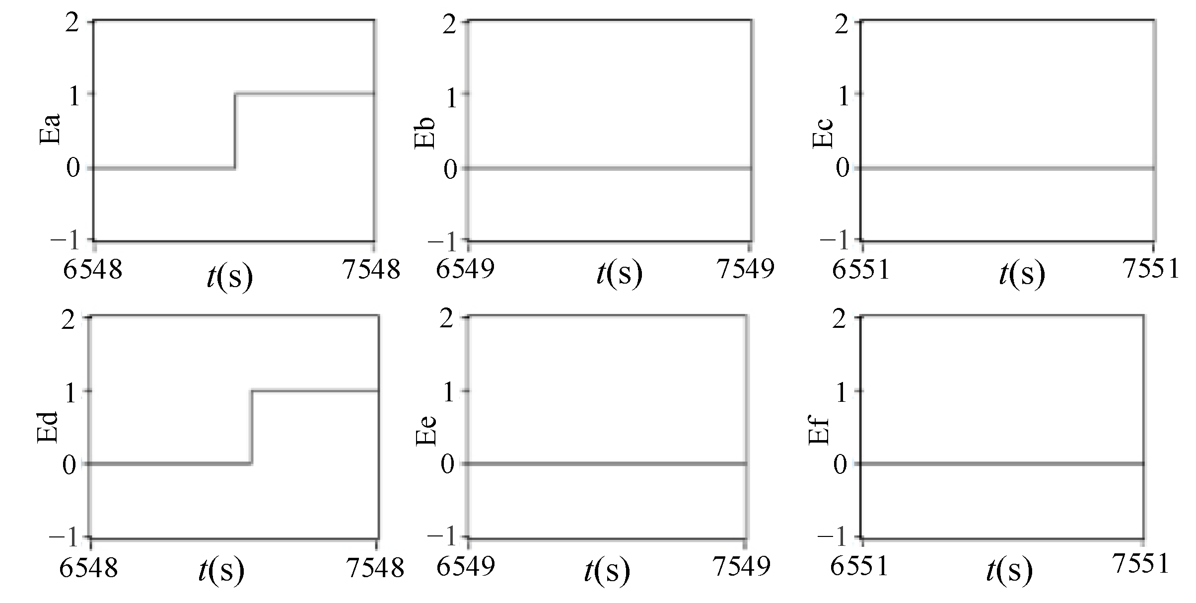
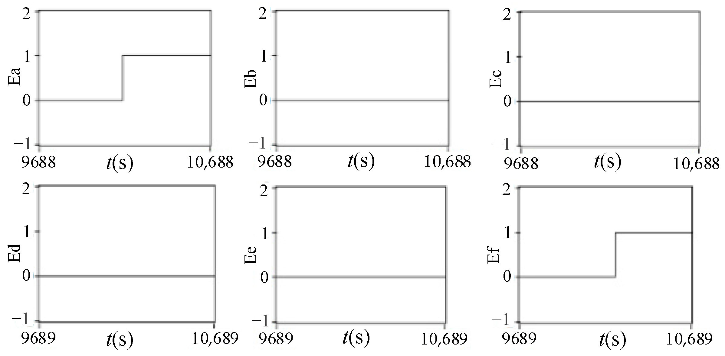
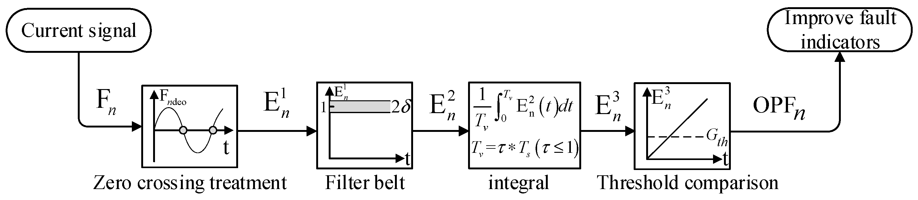
3.1. Calculation of the Phase Failure Index

In the normal state, the fundamental subspace current $i_{\alpha }{,i}_{\beta }$ in the VSD static coordinate system is obtained by decoupling transformation of the six-phase stator current:

$$i_{\alpha }=i_a-\frac{1}{2}{i}_b-\frac{1}{2}{i}_c+\frac{\sqrt{3}}{2}{i}_d-\frac{\sqrt{3}}{2}{i}_e$$

(7)

$$i_{\beta }=\frac{\sqrt{3}}{2}{i}_b-\frac{\sqrt{3}}{2}{i}_c+\frac{1}{2}{i}_d+\frac{1}{2}{i}_e-i_f$$

(8)

Substituting the six-phase stator current of the motor during normal operation into Equations (7) and (8), the following is obtained:

$$\{\begin{array}{l}{i}_{\alpha }=I_{\mathrm{m}}\sin (\theta )-\frac{1}{2}{I}_{\mathrm{m}}\sin (\theta -\frac{2\pi }{3})-\frac{1}{2}{I}_{\mathrm{m}}\sin (\theta +\frac{2\pi }{3})+\frac{\sqrt{3}}{2}{I}_{\mathrm{m}}\sin (\theta -\frac{\pi }{6})-\frac{\sqrt{3}}{2}{I}_{\mathrm{m}}\sin (\theta -\frac{5\pi }{6})=3I_{\mathrm{m}}\sin (\theta )\hfill \\ i_{{}_{\beta }}=\frac{\sqrt{3}}{2}{I}_{\mathrm{m}}\sin (\theta -\frac{2\pi }{3})-\frac{\sqrt{3}}{2}{I}_{\mathrm{m}}\sin (\theta +\frac{2\pi }{3})+\frac{1}{2}{I}_{\mathrm{m}}\sin (\theta -\frac{\pi }{6})+\frac{1}{2}{I}_{\mathrm{m}}\sin (\theta -\frac{5\pi }{6})-I_{\mathrm{m}}\sin (\theta +\frac{\pi }{6})=3I_{\mathrm{m}}\cos (\theta )\hfill \end{array}$$

(9)

Similarly, the current relationship in the harmonic subplane can be obtained:

$$\{\begin{array}{c}{i}_x=i_a-\frac{1}{2}{i}_b-\frac{1}{2}{i}_c-\frac{\sqrt{3}}{2}{i}_d+\frac{\sqrt{3}}{2}{i}_e\\ i_y=-\frac{\sqrt{3}}{2}{i}_b+\frac{\sqrt{3}}{2}{i}_c+\frac{1}{2}{i}_d+\frac{1}{2}{i}_e-i_f\end{array}$$

(10)

Substituting the six-phase stator current of the motor during normal operation into Equation (10) results in:

$$\{\begin{array}{c}{i}_x=0\\ i_y=0\end{array}$$

(11)

It can be deduced from this analysis that the output electromagnetic torque of the motor is mainly provided by the fundamental subspace current components i_α and i_β. In the normal state, the current i_z1, i_z2 of the harmonic subplane is null. The currents i_α,i_β and i_z1,i_z2 after VSD decoupling transformation are shown in Figure 2. The fundamental subspace is circular in the steady-state current i_α,i_β. The harmonic subspace current i_z1,i_z2 is the point at the origin, which is coherent with the theoretical calculation results.

By inverting the normal VSD transformation, the following is obtained:

$$\left[\begin{array}{c}{i}_a\\ i_b\\ i_c\\ i_d\\ i_e\\ i_f\end{array}\right]=\frac{1}{\sqrt{3}}\left[\begin{array}{cccccc}1& 0& 1& 0& 1& 0\\ -\raisebox{1ex}{$1$}\!\left/ \!\raisebox{-1ex}{$2$}\right.& \raisebox{1ex}{$\sqrt{3}$}\!\left/ \!\raisebox{-1ex}{$2$}\right.& -\raisebox{1ex}{$1$}\!\left/ \!\raisebox{-1ex}{$2$}\right.& -\raisebox{1ex}{$\sqrt{3}$}\!\left/ \!\raisebox{-1ex}{$2$}\right.& 1& 0\\ -\raisebox{1ex}{$1$}\!\left/ \!\raisebox{-1ex}{$2$}\right.& -\raisebox{1ex}{$\sqrt{3}$}\!\left/ \!\raisebox{-1ex}{$2$}\right.& -\raisebox{1ex}{$1$}\!\left/ \!\raisebox{-1ex}{$2$}\right.& \raisebox{1ex}{$\sqrt{3}$}\!\left/ \!\raisebox{-1ex}{$2$}\right.& 1& 0\\ \raisebox{1ex}{$\sqrt{3}$}\!\left/ \!\raisebox{-1ex}{$2$}\right.& \raisebox{1ex}{$1$}\!\left/ \!\raisebox{-1ex}{$2$}\right.& -\raisebox{1ex}{$\sqrt{3}$}\!\left/ \!\raisebox{-1ex}{$2$}\right.& \raisebox{1ex}{$1$}\!\left/ \!\raisebox{-1ex}{$2$}\right.& 0& 1\\ -\raisebox{1ex}{$\sqrt{3}$}\!\left/ \!\raisebox{-1ex}{$2$}\right.& \raisebox{1ex}{$1$}\!\left/ \!\raisebox{-1ex}{$2$}\right.& \raisebox{1ex}{$\sqrt{3}$}\!\left/ \!\raisebox{-1ex}{$2$}\right.& 0& 0& 1\\ 0& -1& 0& -1& 0& 1\end{array}\right]\left[\begin{array}{c}{i}_{\alpha }\\ i_{\beta }\\ i_{z1}\\ i_{z2}\\ i_{o1}\\ i_{o2}\end{array}\right]$$

(12)

When a phase failure occurs, it can be seen from Equation (12) that the fundamental and harmonic plane currents have a certain relationship. It is assumed that the phase failure of phase a winding occurs. That is, when the constraint condition is i_a = 0, the first row of the VSD inverse matrix (cf. Equation (12)) is multiplied by the plane current in order to obtain i_α + i_z1 = 0. When the motor is in normal operation, the harmonic current is i_z1 = 0. In summary, the open circuit fault index F_a can be computed as:

$${\mathrm{F}}_a=-\frac{i_{z1}}{i_{\alpha }}$$

(13)

Similarly, the open-circuit fault index of six-phases (cf. Equation (14)) can be obtained:

$$\{\begin{array}{c}{\mathrm{F}}_a=-\frac{i_{z1}}{i_{\alpha }}\\ {\mathrm{F}}_b=\frac{i_{z1}}{-i_a+\sqrt{3}{i}_{\beta }-\sqrt{3}{i}_{z2}}\\ {\mathrm{F}}_c=\frac{i_{z1}}{-i_a-\sqrt{3}{i}_{\beta }+\sqrt{3}{i}_{z2}}\\ {\mathrm{F}}_d=\frac{i_{z1}}{i_a+1/\sqrt{3}{i}_{\beta }+1/\sqrt{3}{i}_{z2}}\\ {\mathrm{F}}_e=\frac{i_{z1}}{i_a-1/\sqrt{3}{i}_{\beta }-1/\sqrt{3}{i}_{z2}}\\ {\mathrm{F}}_f=-\frac{i_{z2}}{i_{\beta }}\end{array}$$

(14)

The numerator of this fault index is the harmonic plane current. Due to the fact that the harmonic plane current component is null in the normal state, the fault index is always kept null during the normal operation of the motor. When a phase fault occurs, the fault index of the phase rises 1, so as to distinguish the normal operation and inverter phase fault.

3.2. Optimization Scheme of the Winding Open Circuit Fault Index

In the case where only the fault index F_n (n = a,b,c,d,e,f) is used, because the denominator of the fault indicator is too small near the zero-crossing area, a spike pulse will appear, which may lead to misdiagnosis. Therefore, the fault index F_n should be improved and optimized. The optimization process is illustrated in Figure 3.

The fault index F_n is first subjected to peak pulse processing using Equation (15), in order to obtain the first fault index ${\mathrm{E}}_n^1:$

$$\{\begin{array}{c}{\mathrm{E}}_n^1=0_{},\left|{\mathrm{F}}_{ndeo}\right|\le \Delta \\ {\mathrm{E}}_n^1{=\mathrm{F}}_n,\left|{\mathrm{F}}_{ndeo}\right|>\Delta \end{array}$$

(15)

where F_ndeo is the denominator value of fault index F_n and ∆ is the threshold value of the zero-crossing area width. This value cannot be too large, in order to ensure the diagnosis speed. The specific value is determined according to the experiment. In this paper, ∆ is set to 0.1.

The fault index after peak pulse processing is then filtered using Equation (16) in order to obtain the second fault index ${\mathrm{E}}_n^2$:

$$\{\begin{array}{l}{\mathrm{E}}_n^2{=\mathrm{E}}_n^1,(1-\delta \le {\mathrm{E}}_n^1\le 1+\delta )\hfill \\ {\mathrm{E}}_n^2=0 ,(1+\delta \le {\mathrm{E}}_n^1\&{\mathrm{E}}_n^1\le 1-\delta )\hfill \end{array}$$

(16)

where δ is the width of the filter band, which is used to filter out the unnecessary interference while not affecting the subsequent processing. The recommended value range of δ is [0.1–0.3]. In this paper, it is set to 0.1.

The processed fault index will be set to 1 after the fault occurs. However, the fault index will be set to zero in the zero-crossing area, due to the processing of the zero-crossing spike pulse. Therefore, it is necessary to integrate the fault index according to Equation (17) in order to obtain the third fault index ${\mathrm{E}}_n^3$:

$${\mathrm{E}}_n^3=\frac{1}{{\mathrm{T}}_{\mathrm{v}}}{\displaystyle {\int }_0^{{\mathrm{T}}_{\mathrm{v}}}{\mathrm{E}}_n^2\left(t\right)}\mathrm{d}t$$

(17)

$${\mathrm{T}}_{\mathrm{v}}=\tau \ast {\mathrm{T}}_{\mathrm{s}}\left(\tau \le 1\right)$$

(18)

where T_s is the periodic value of the current fundamental wave. The larger the value of τ, the slower the diagnosis speed, but the higher the diagnosis accuracy. On the contrary, the smaller the value of τ, the faster the diagnosis speed, but the smaller the diagnosis accuracy. In this paper, τ is set to 0.6, in order to ensure the diagnosis accuracy and rapidity. The traditional integration consists in integrating the fault indicators of the whole cycle, which will prolong the fault diagnosis time and reduce the diagnosis efficiency. Selecting T_v Equation (18) can speed up the detection speed.

Finally, the third fault index ${\mathrm{E}}_n^3$ is compared with the threshold in order to obtain the improved fault index OPF_n:

$$\{\begin{array}{c}{\mathrm{OPF}}_n=1, {\mathrm{E}}_n^3>{\mathrm{G}}_{th}\\ {\mathrm{OPF}}_n=0, {\mathrm{E}}_n^3<{\mathrm{G}}_{th}\end{array}$$

(19)

where G_th is the judgment threshold selected between 0 and 1. If the value of G_th is too large, the diagnosis speed will slow down. Because these steps have a negative integration link to suppress the fluctuation of fault indicators, the value can be appropriately reduced, and G_th can have a value between 0.1 and 0.3.

It can be deduced that using the constraint condition that the fault phase current is null after the phase failure, combined with the vector space decoupled VSD inverse matrix, the fault index of the phase failure is derived. This can diagnose and locate 15 types of phase faults of the inverter, including 6 types of single-phase faults and 9 types of two-phase faults of different windings.

4. Power Switch Fault Diagnosis Strategy

Several types of power switch faults exist. They mainly include the short circuit and open circuit faults. The short circuit fault has a short duration and is difficult to detect. For further treatment, the short circuit fault is changed into open an circuit fault by a fuse device. The open-circuit faults are mostly single-switch and two-switch faults. The fault of two switches on the same bridge arm can be treated as open phase fault. Therefore, this paper only tackles the open circuit fault of a single switch and two switches on different bridge arms.

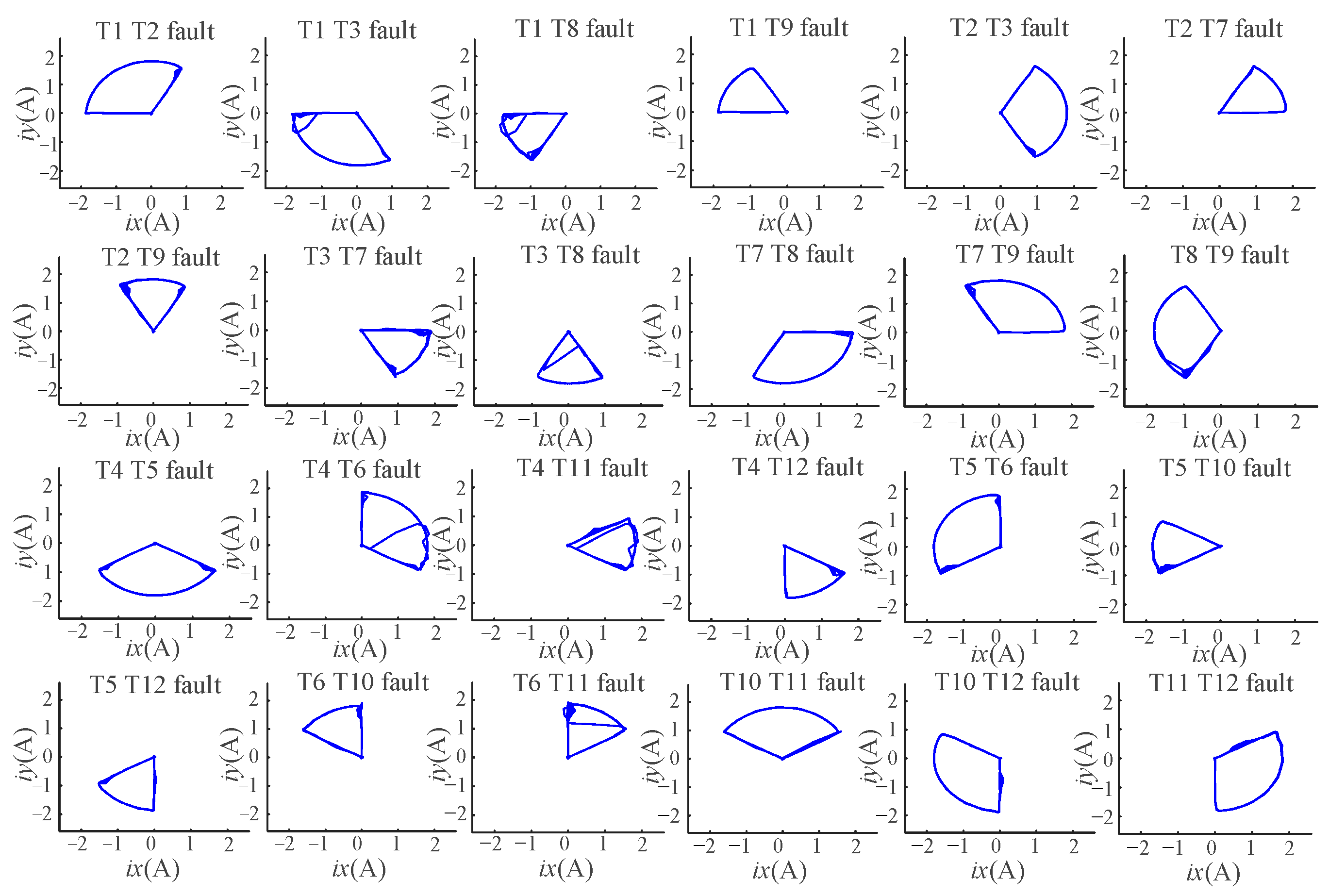
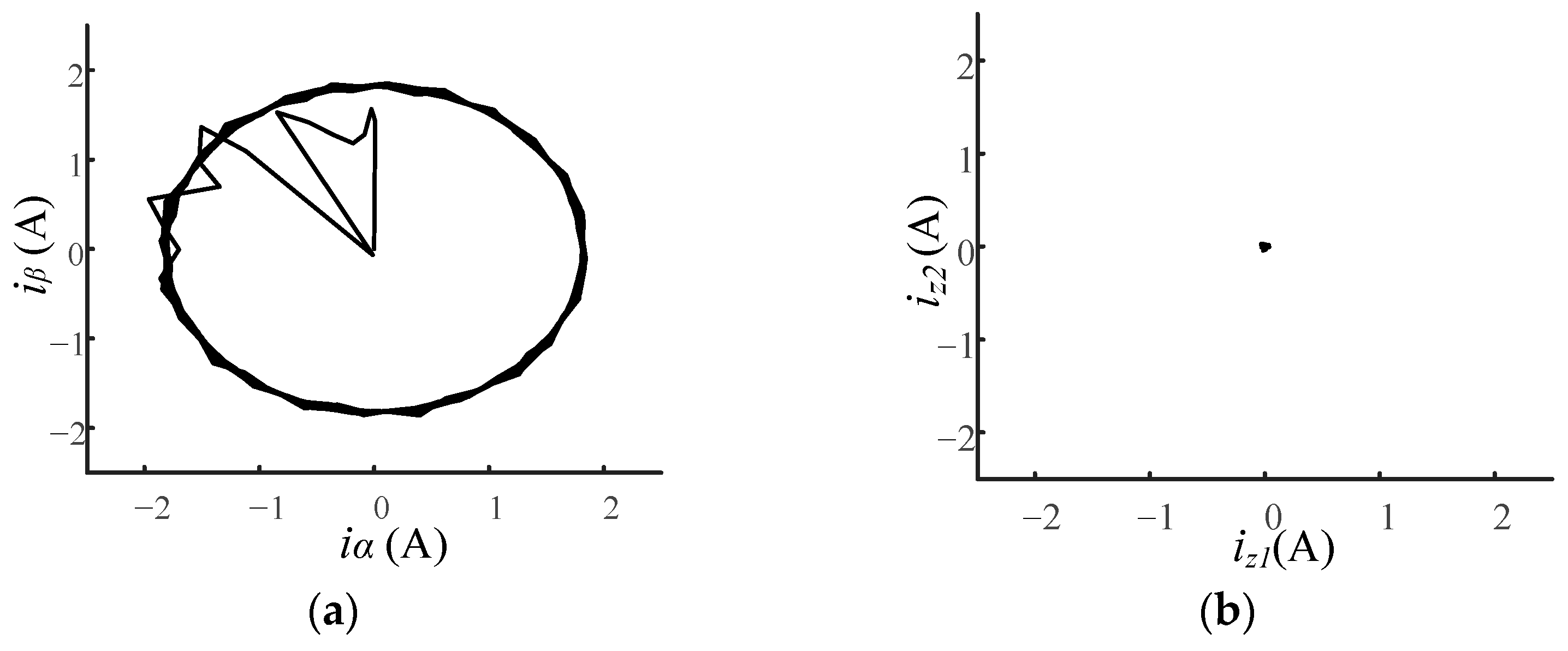
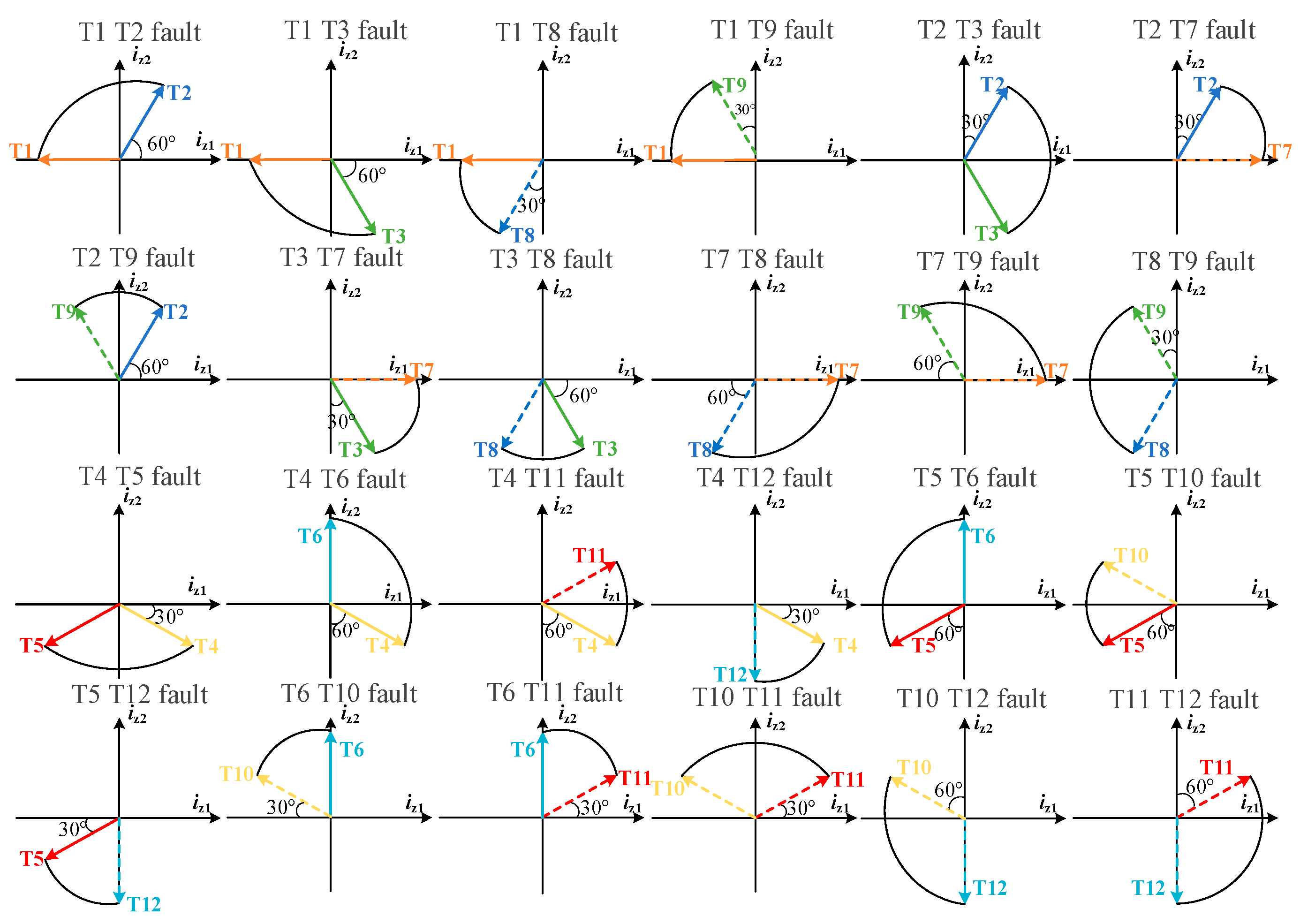
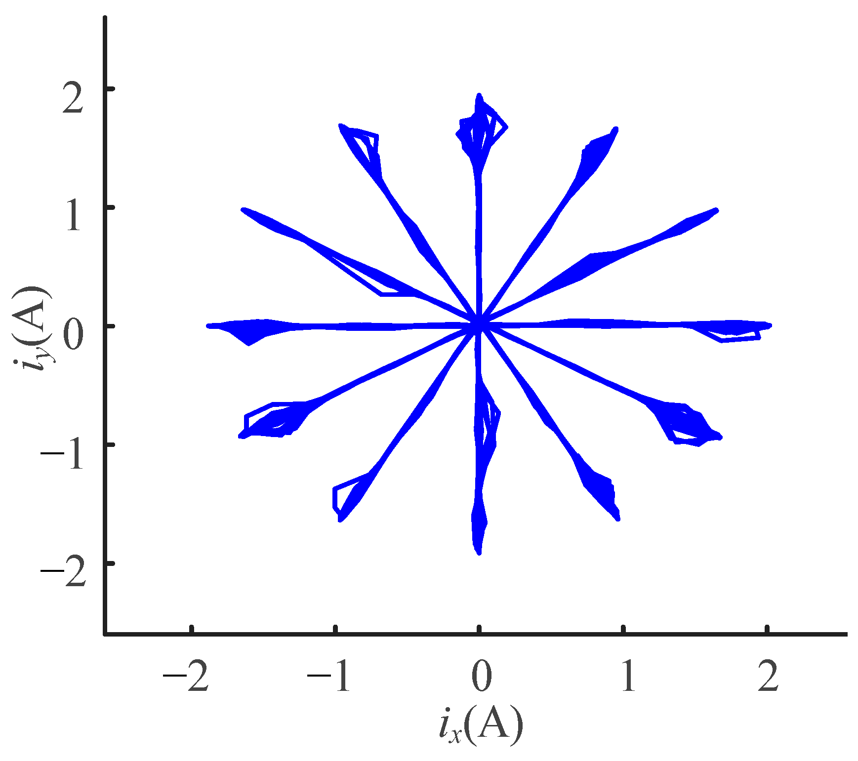
4.1. Harmonic Plane Current Fault Trace Analysis

Figure 4 shows the current waveform of the z₁-z₂ plane when different switches fail after VSD conversion of the six-phase stator current. When T1 fails, the current trajectory of the z₁-z₂ plane points to the negative half of the z₁ axis. When T1 and T2 fail, the current trajectories of i_z1 and i_z2 are fan-shaped. Similarly, when other switches fail, they also have these trajectory characteristics.

The reference direction of the current vector during each phase fault can be expressed as:

$$\mathrm{dn}-\mathrm{ref}=\arctan (\frac{{\mathrm{A}}_{z2}}{{\mathrm{A}}_{z1}})\{\begin{array}{l}\pi -(k-1)\frac{\pi }{6},f_n\le 1\hfill \\ -(k-1)\frac{\pi }{6},f_n\ge 0\hfill \end{array}$$

(20)

where A_z1 and A_z2 represent the amplitude of harmonic currents i_z1 and i_z2, respectively. n represents the a,b,c,d,e,f phase, while the fault phase corresponding to k = 1, 5, −3, −4, 6, 4 is a,b,c,d,e,f, respectively. The fault current vector turns counterclockwise by angle dn-ref from the x axis. $f_n\left(t\right)={\int }_0^{\mathrm{T}}{i}_{n}dt$ is the average value of fault current in a current cycle.

It can be deduced that in the case of a single-switch or two-switch open-circuit fault of the inverter, the current trajectory in the harmonic i_z1 and i_z2 planes regularly changes. The current vector trajectory profile under single-switch and multi-switch faults can be developed using the current values in the i_z1 and i_z2 harmonic planes, as shown in Figure 5 and Figure 6.

According to the different reference directions of the current track under the z₁-z₂ plane fault, the intelligent algorithm has the characteristics of strong analysis ability and several diagnosis types. Therefore, the neural network algorithm is used for fault diagnosis based on the characteristics of fault current trajectory.

In order to distinguish the fault types and improve the diagnosis efficiency, different fault types should be classified and coded. The 12 bit binary number F₁F₂F₃F₄F₅F₆F₇F₈F₉F₁₀F₁₁F₁₂ is used to encode the single-switch and two-switch faults of the six-phase inverter. When all the bits are equal to 1, the switch has an open-circuit fault. On the contrary, when all the bits are 0, the switch has no fault. Note that there are 36 fault conditions. The specific fault types are shown in

Table 1. Fault type code.

Fault Switch	Fault Type	Fault Code	Fault Switch	Fault Type	Fault Code
Nothing	Normal	000000000000
T1	Single-switch fault of the first set of winding	100000000000	T4	Single-switch fault of the second set of winding	000100000000
T2		010000000000	T5		000010000000
T3		001000000000	T6		000001000000
T7		000000100000	T10		000000000100
T8		000000010000	T11		000000000010
T9		000000001000	T12		000000000001
T1T2	Failure of two switches of the first set of winding	110000000000	T4T5	Failure of two switches of the second set of winding	000110000000
T1T3		101000000000	T4T6		000101000000
T1T8		100000010000	T4T11		000100000010
T1T9		100000001000	T4T12		000100000001
T2T3		011000000000	T5T6		000011000000
T2T7		010000100000	T5T10		000010000100
T2T9		010000001000	T5T12		000010000001
T3T7		001000100000	T6T10		000001000100
T3T8		001000010000	T6T11		000001000010
T7T8		000000110000	T10T11		000000000110
T7T9		000000101000	T10T12		000000000101
T8T9		000000011000	T11T12		000000000011

.

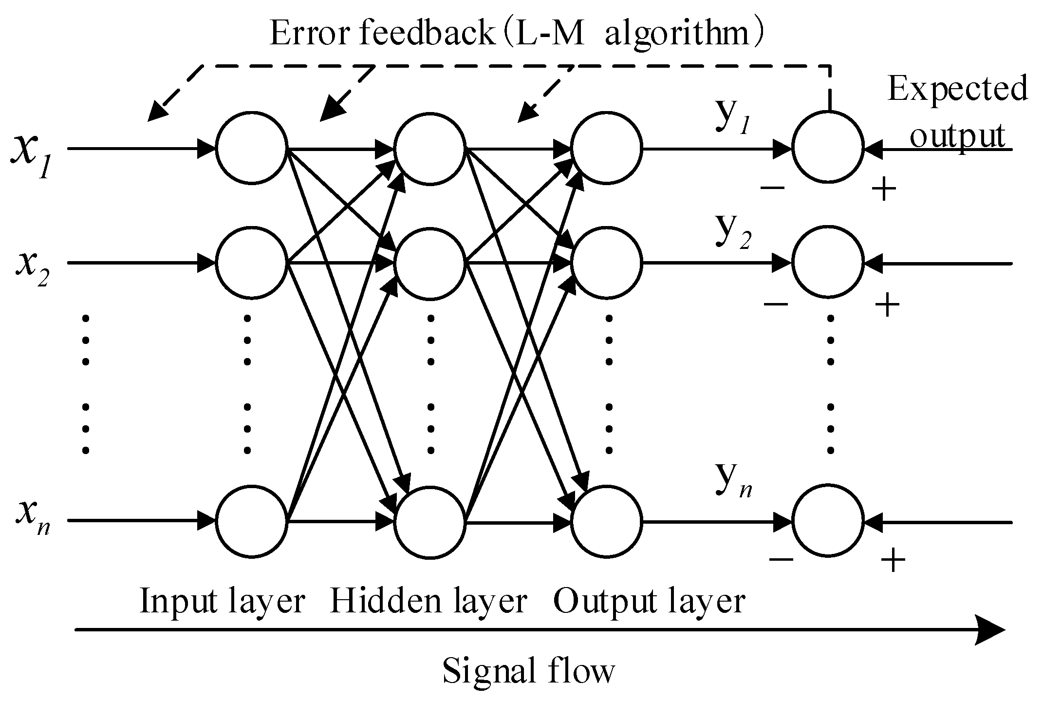
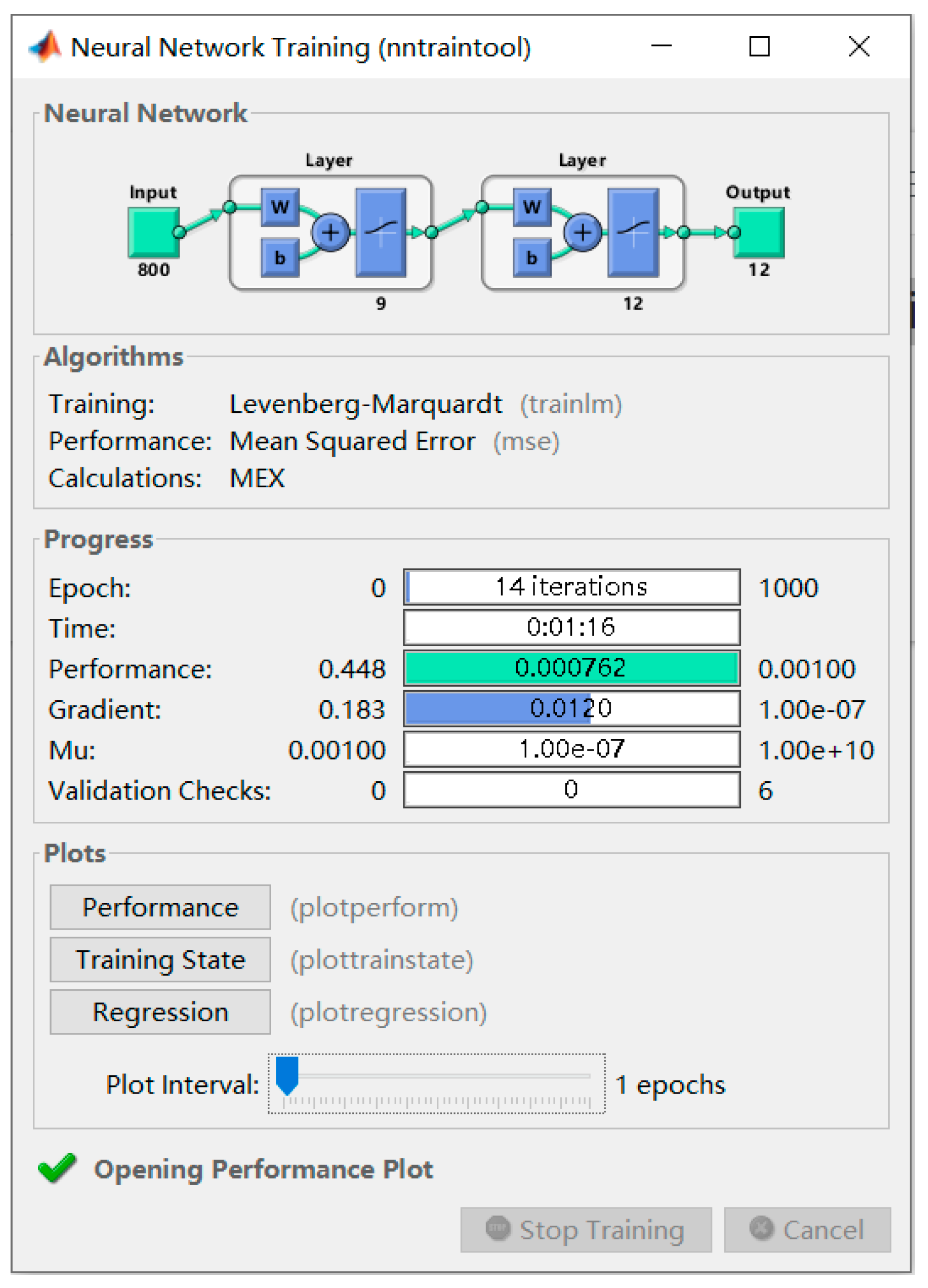
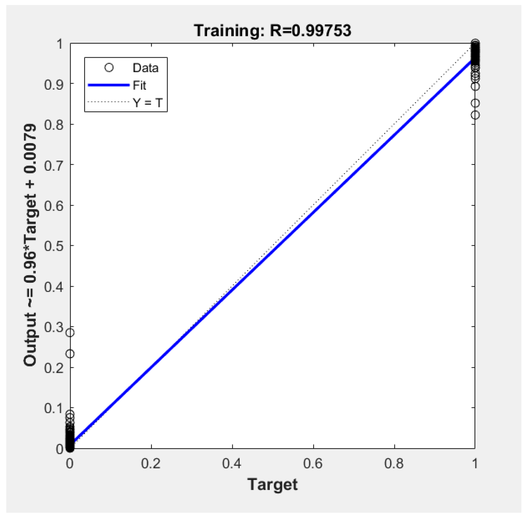
4.2. Principle and Algorithm of BP Neural Network

The neural network is a nonlinear system. Each neuron can output a signal according to the input layer signal and activation function. In addition, a large number of neurons can jointly form a highly nonlinear system [23]. Figure 7 presents a representative neuron structure model.

In the latter, x₁,x₂,x₃…x_n is the input parameter, W_k1, W_k2, W_k3…W_k(n−1), W_kn represents the weight of each parameter, ${\theta }_i$ denotes the threshold, f(·) s the activation function, and y_i represents the neuron output. The relationship between each variable is given by:

$$\{\begin{array}{l}{u}_i={\displaystyle \sum _{j=1}^n{w}_{ij}}{x}_j\hfill \\ v_i=u_i+\theta \hfill \end{array}$$

(21)

The output y_i of the neuron is expressed as:

$$y_i=f\left({\displaystyle \sum _{j=1}^n{w}_{ij}}{x}_j+{\theta }_i\right)$$

(22)

The structure of the BP neural network is shown in Figure 8. Due to the gradient descent method, the training can fall into the local minimum, which leads to the inability of effective training [24]. Therefore, this paper uses the Levenbrg–Marquardt algorithm based on the combination of the gradient method and Newton method, in order to optimize the BP neural network. This method has less iterations and a fast iteration speed. Therefore, it can approach the optimal weight faster in order to complete the training.

Considering that the residual of the output layer is γ(x), which has a nonlinear relationship with x, the iterative formula of the Gauss Newton method is given by:

$$\{\begin{array}{l}{x}_{k+1}=x_k+\Delta x_{gn}\hfill \\ x_{k+1}=x_k-H^{-1}\nabla f\hfill \end{array}$$

(23)

where ∇f and H are respectively the gradient and Hessian matrix of γ(x) given by:

$$\begin{array}{l}\nabla f=2J_r^{T}r=2{\displaystyle \sum _{i=1}^m{r}_i\frac{\delta r_i}{\delta x_i}}\\ H_{jk}=2J_r^T{J}_r=2{\displaystyle \sum _{i=1}^m\left(\frac{\delta r_i}{\delta x_j}\frac{\delta r_i}{\delta x_k}+r_i\frac{{\partial }^2{r}_i}{\partial x_j\partial x_k}\right)}\end{array}$$

(24)

and therefore:

$$\Delta x_{gn}=-{(J_r^T{J}_r)}^{-1}{J}_r^{T}r$$

(25)

The Levenbrg–Marquardt algorithm improves the iteration step size:

$$y_i=f\left({\displaystyle \sum _{j=1}^n{w}_{ij}}{x}_j+{\theta }_i\right)$$

(26)

where I is the identity matrix and μ represents the damping factor usually having a value range of [10⁻⁸, 1], which ensures that $J_r^T{J}_r+\mu \mathrm{I}$ is a positive definite matrix and that the iteration is in the downward direction.

Before using the neural network diagnosis, the relevant parameters of the neural network should be set according to the needs, the Sigmoid function should be selected as the activation function, the three-layer neural network should be used for training, and the other parameters should be set by default.

5. Simulation Analysis

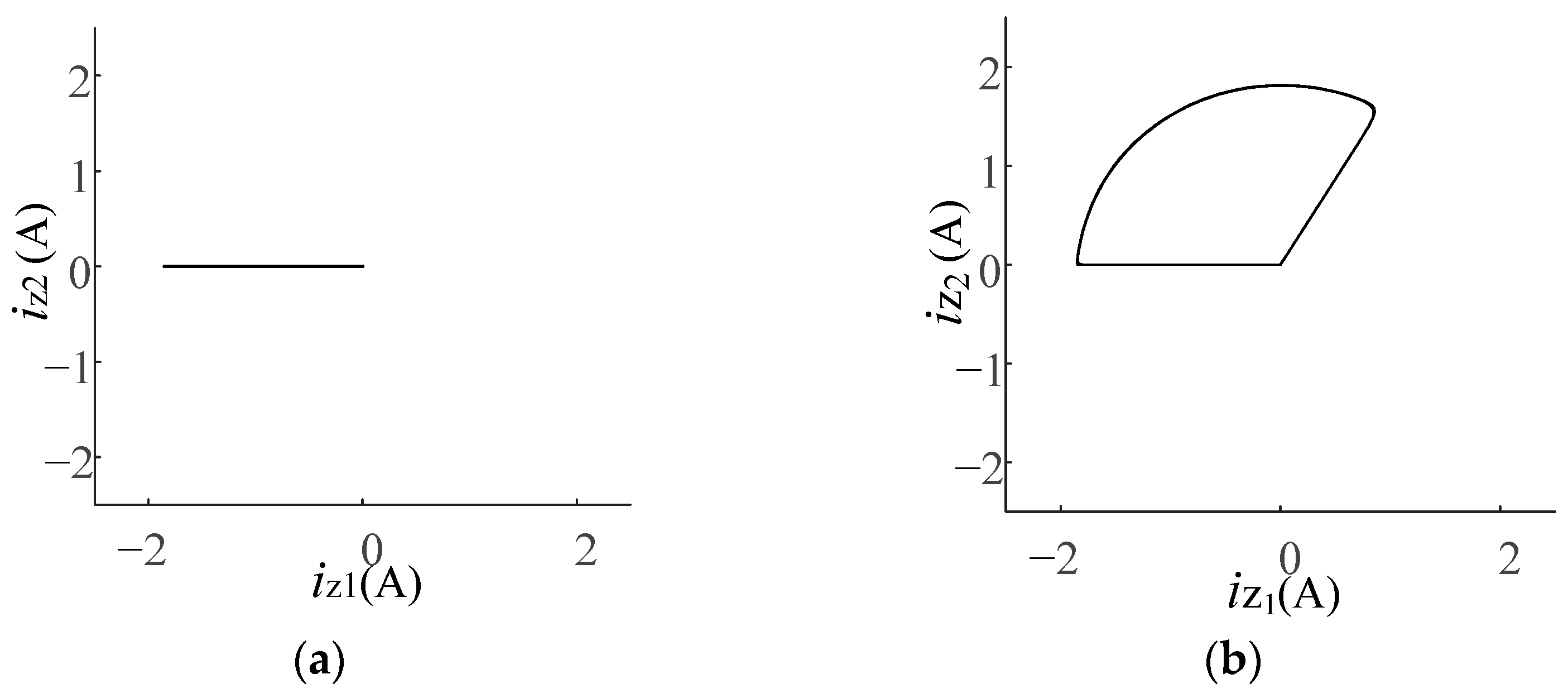
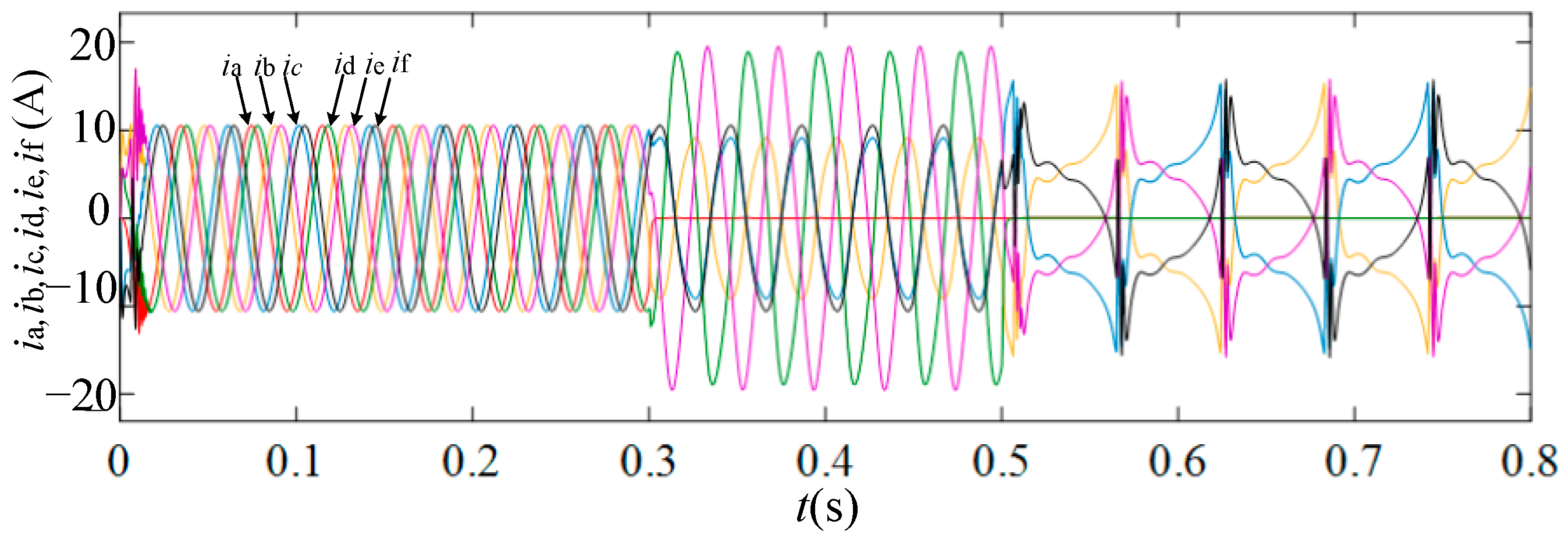
5.1. Simulation Analysis of Winding Open-Circuit Fault

In order to verify the proposed fault diagnosis algorithm, a six-phase motor simulation model is built, which is mainly composed of a rectifier, controller, inverter, and motor. The motor parameters are: rated output power P = 10 kW, rated voltage U = 311 V, rated current I = 20 A, rated speed N = 1500 r/min, rated torque T = 60 N·m, pole pair p = 5, quadrature axis and direct axis inductance L_d = L_q = 8.5 mH, and power factor = 0.9.

The current waveform obtained by increasing and decreasing load and disturbance under normal conditions of the motor is shown in Figure 9. After the motor speed is increased, the load is set to 30 N·m and runs stably at 500 r/min. The six-phase stator current waveform is balanced and the sinusoidal degree is satisfactory. When the load of the motor suddenly changes to 45 N·m at 0.2 s, the current amplitude rapidly increases and runs in a stable state. When the load decreases to 40 N·m at 0.4 s, the current decreases. When the interference is added at 0.6 s, the motor current slightly increases and then decreases to the stable state.

The fault index waveform corresponding to this case is shown in Figure 10. The fault index of the six-phase open circuit is null. In addition, there is no rise when the motor stably operates, suddenly increases or decreases load, and suddenly adds disturbance. The fault index has no false diagnosis under different conditions without fault, which proves that the diagnosis method has a good robustness.

The current waveform of the open-circuit fault of phase a at 0.3 s is shown in Figure 11. The load torque is 30 N·m, and the phase failure of phase a occurs at 0.3 s. The phase a current becomes zero after 0.3 s. Among the remaining four-phase currents, phase b and phase c have the same amplitude and complementary waveforms, and the waveform amplitude and phase of phase d, e and f change to varying degrees.

The fault index waveform under these conditions is shown in Figure 12. After 0.3 s, the phase a fault index rises to 1 and the fault indexes of other phases do not change.

The current waveform of the open-circuit fault of phase a and phase d at 0.3 s and 0.5 s is shown in Figure 13. The load torque is 30 N·m, the phase failure of phase a and phase d occurs at 0.3 s and 0.5 s, respectively. The phase a current becomes zero after 0.3 s and the phase d current also becomes zero after 0.5 s.

The fault index waveform under these conditions is shown in Figure 14. After 0.3 s, the phase a fault index rises to 1, and the phase d fault index rapidly rises to 1 within the second half cycle of 0.5 s, so as to accurately locate the two-phase open-circuit fault.

The current waveform of the open-circuit fault of phase a and phase f at 0.3 s and 0.5 s is shown in Figure 15. The load torque is 30 N·m, the phase failure of phase a and phase f occurs at 0.3 s and 0.5 s, respectively. The phase a current becomes zero after 0.3 s and the phase f current also becomes zero after 0.5 s. Among the remaining four-phase currents, phase b and phase c have the same amplitude and opposite phase. Similarly, phase d and phase e have the same amplitude and opposite phase.

The fault index waveform under these conditions is shown in Figure 16. After 0.3 s, the phase a fault index rises to 1, and the phase f fault index rapidly rises to 1 within the second half cycle of 0.5 s, so as to accurately locate the two-phase open-circuit fault.

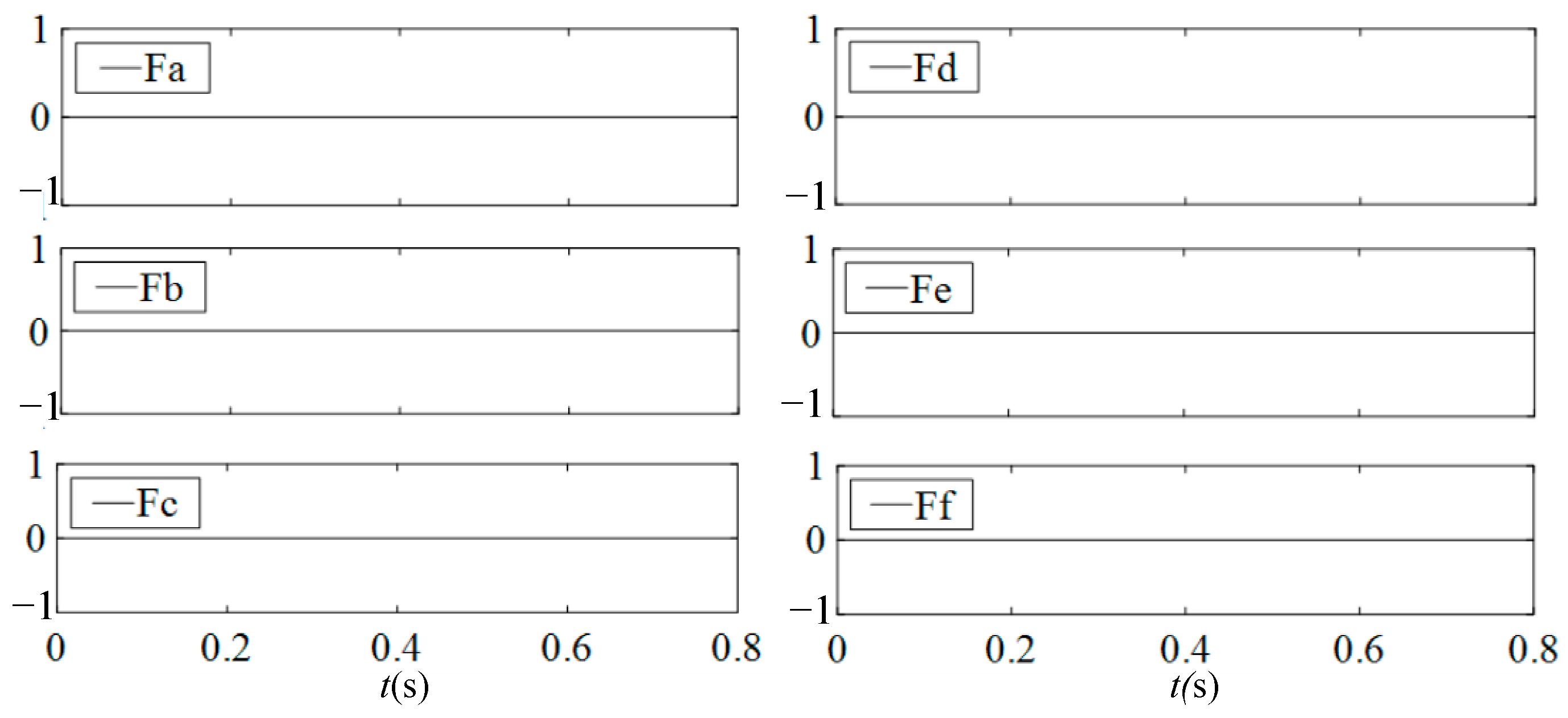
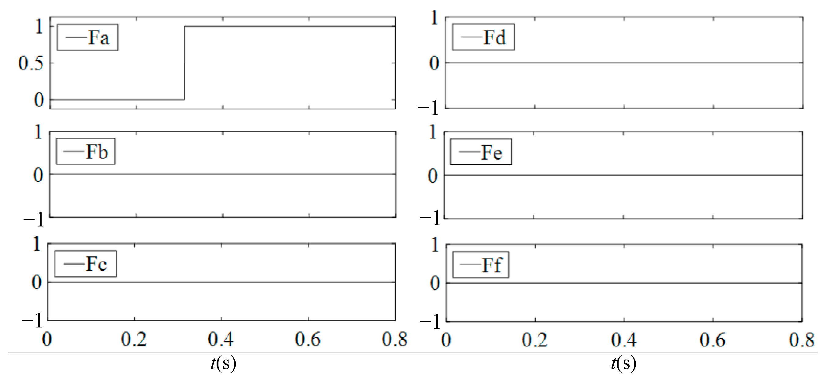
5.2. Switch Fault Simulation

Figure 17 shows the harmonic plane current trajectories obtained by simulation in the case of 12 single-switch faults. It can be observed that the fault trajectories of the 12 switches of the six-phase VSI inverter are consistent with the theory.

Figure 18 illustrates the harmonic plane current trajectories obtained by simulation, in the case of 24 types of two-switch faults. The harmonic plane current trajectories are fan-shaped patterns with different center angles in the case of two-switch faults, that are used as characteristic signals for fault diagnosis.

Figure 19 presents the training model of the neural network. The current vector characteristic trajectories of single-switch fault and two-switch fault, are used as samples for training. The hidden layer neuron is 9, the expected error is 0.001, and the maximum number of iterations is 1000. The Newff function is used for training and the Sigmoid function is used as the activation function. The feedback process of the optimization error is performed using the L–M algorithm.

Figure 20 shows the training error convergence curve of the neural network. The neural network optimized using the L–M algorithm has a high convergence speed. When the training is completed 14 times, the mean square error is 7.6208 × 10⁻⁴, which meets the error requirements.

The coincidence degree between the error regression curve and the expected curve shown in Figure 21 is high. This proves that the neural network has good fitting and classification ability for different fault current trajectories.

The diagnosis results of the neural network are shown in

Table 2. Neural network diagnosis results.

Serial Number	Actual Output	Ideal Output	Fault Type
1	0.9574 0.0003 0.0923 0.0119 0.0492 0.0087 0.0029 0.0565 0.0984 0.0278 0.0106 0.0012	100000000000	T1
2	0.0094 0.9869 0.0147 0.0131 0.0106 0.0236 0.0293 0.0001 0.0882 0.0017 0.0453 0.0031	010000000000	T2
3	0.0895 0.0282 0.9365 0.0013 0.0003 0.0002 0.0718 0.1507 0.0004 0.0077 0.0002 0.0221	001000000000	T3
4	0.0016 0.0000 0.0071 0.9399 0.0615 0.0297 0.0001 0.0578 0.0000 0.0313 0.0001 0.0373	000100000000	T4
5	0.0002 0.0181 0.0001 0.0198 0.9987 0.0001 0.0003 0.0001 0.0000 0.0001 0.2961 0.0052	000010000000	T5
6	0.0068 0.0009 0.0001 0.0384 0.0000 0.9631 0.0064 0.0002 0.0103 0.0000 0.0200 0.0000	000001000000	T6
7	0.0010 0.0060 0.0217 0.0580 0.1198 0.0036 0.9840 0.0385 0.0447 0.0691 0.0316 0.0005	000000100000	T7
8	0.1813 0.0000 0.0052 0.0019 0.0398 0.0241 0.0077 0.9211 0.0005 0.0055 0.0000 0.0904	000000010000	T8
9	0.0049 0.0096 0.0003 0.0111 0.0893 0.0558 0.0040 0.0764 0.9695 0.1351 0.0002 0.0058	000000001000	T9
10	0.0156 0.0001 0.0099 0.0003 0.085 0.0324 0.0000 0.0054 0.0009 0.9973 0.0001 0.0237	000000000100	T10
11	0.0000 0.0019 0.0021 0.0021 0.0055 0.0009 0.0001 0.0000 0.0014 0.6796 0.9954 0.0058	000000000010	T11
12	0.0137 0.0000 0.0233 0.0171 0.0014 0.0001 0.0244 0.0005 0.0000 0.0001 0.0227 0.9101	000000000001	T12
13	0.9455 0.9961 0.0199 0.0014 0.0007 0.0059 0.0699 0.0720 0.0533 0.0006 0.0000 0.0012	110000000000	T1T2
14	0.9635 0.0585 0.9787 0.0003 0.0013 0.0002 0.1210 0.0322 0.0418 0.1409 0.0006 0.0002	101000000000	T1T3
15	0.9465 0.0002 0.0262 0.0004 0.0414 0.0618 0.0002 0.9202 0.0022 0.0302 0.0000 0.0214	100000010000	T1T8
16	0.9799 0.1623 0.0730 0.0002 0.0022 0.0116 0.0092 0.0692 0.9608 0.1598 0.0000 0.0007	100000001000	T1T9
17	0.0247 0.9807 0.9339 0.0015 0.0016 0.0001 0.0754 0.0216 0.0840 0.0010 0.0391 0.0007	011000000000	T2T3
18	0.0001 0.9602 0.0222 0.0063 0.0264 0.0007 0.9491 0.0050 0.0870 0.0007 0.0175 0.0411	010000100000	T2T7
19	0.0004 0.9792 0.0095 0.0001 0.0016 0.0549 0.0009 0.0012 0.9561 0.0095 0.0141 0.0937	010000001000	T2T9
20	0.0479 0.0051 0.9673 0.0080 0.0000 0.0008 0.9701 0.0603 0.0000 0.0512 0.0000 0.0003	001000100000	T3T7
21	0.0076 0.0000 0.9344 0.0029 0.0003 0.0068 0.0003 0.9902 0.0001 0.0724 0.0958 0.0069	001000010000	T3T8
22	0.0000 0.0000 0.0195 0.9876 0.8665 0.0032 0.0001 0.0001 0.0000 0.0051 0.0507 0.0106	000110000000	T4T5
23	0.0002 0.0186 0.0001 0.9968 0.0311 0.9535 0.0064 0.0002 0.0000 0.0000 0.0366 0.0000	000101000000	T4T6
24	0.0000 0.0092 0.0005 0.9422 0.0242 0.0008 0.0000 0.0008 0.0000 0.0036 0.9658 0.0414	000100000010	T4T11
25	0.0000 0.0000 0.0051 0.9606 0.0115 0.0004 0.0428 0.0034 0.0000 0.0009 0.0274 0.9119	000100000001	T4T12
26	0.0002 0.0494 0.0000 0. 0011 0.8858 0.9982 0.0017 0.0001 0.0032 0.0001 0.0969 0.0000	000011000000	T5T6
27	0.1324 0.0013 0.0000 0.0000 0.9892 0.0006 0.0000 0.0357 0.0004 0.8010 0.0008 0.0048	000010000100	T5T10
28	0.0001 0.0001 0.0122 0.1004 0.9647 0.0000 0.0021 0.0003 0.0000 0.0363 0.0163 0.7030	000010000001	T5T12
29	0.0315 0.0002 0.0368 0.0010 0.0001 0.9669 0.0163 0.0004 0.0328 0.8387 0.0001 0.0033	000001000100	T6T10
30	0.0000 0.0015 0.0001 0.1827 0.0001 0.6872 0.0673 0.0000 0.0026 0.0000 0.9825 0.0000	000001000010	T6T11
31	0.0050 0.0000 0.1506 0.0274 0.0174 0.0003 0.9406 0.9372 0.0022 0.0685 0.0001 0.0021	000000110000	T7T8
32	0.0724 0.0930 0.0004 0.0007 0.0014 0.0508 0.9778 0.1332 0.9280 0.0191 0.0000 0.0002	000000101000	T7T9
33	0.0837 0.0270 0.0092 0.0007 0.0446 0.0027 0.0275 0.9727 0.9892 0.1027 0.0000 0.0011	000000011000	T8T9
34	0.0000 0.0000 0.0401 0.0074 0.0001 0.0153 0.0005 0.0002 0.0005 0.9980 0.6568 0.1243	000000000110	T10T11
35	0.0002 0.0001 0.0033 0.1092 0.1596 0.0033 0.0033 0.0407 0.0000 0.9995 0.0083 0.9203	000000000101	T10T12
36	0.0008 0.0044 0.0451 0.0283 0.0005  0.0000 0.0014 0.0002 0.0000 0.0009 0.9609 0.9795	000000000011	T11T12

. It can be seen that the trained network can identify the single-switch and two-switch faults. The error between the output value of 12 neurons in the output layer and the coding value of the fault type is very small, which leads to an accurate diagnosis.

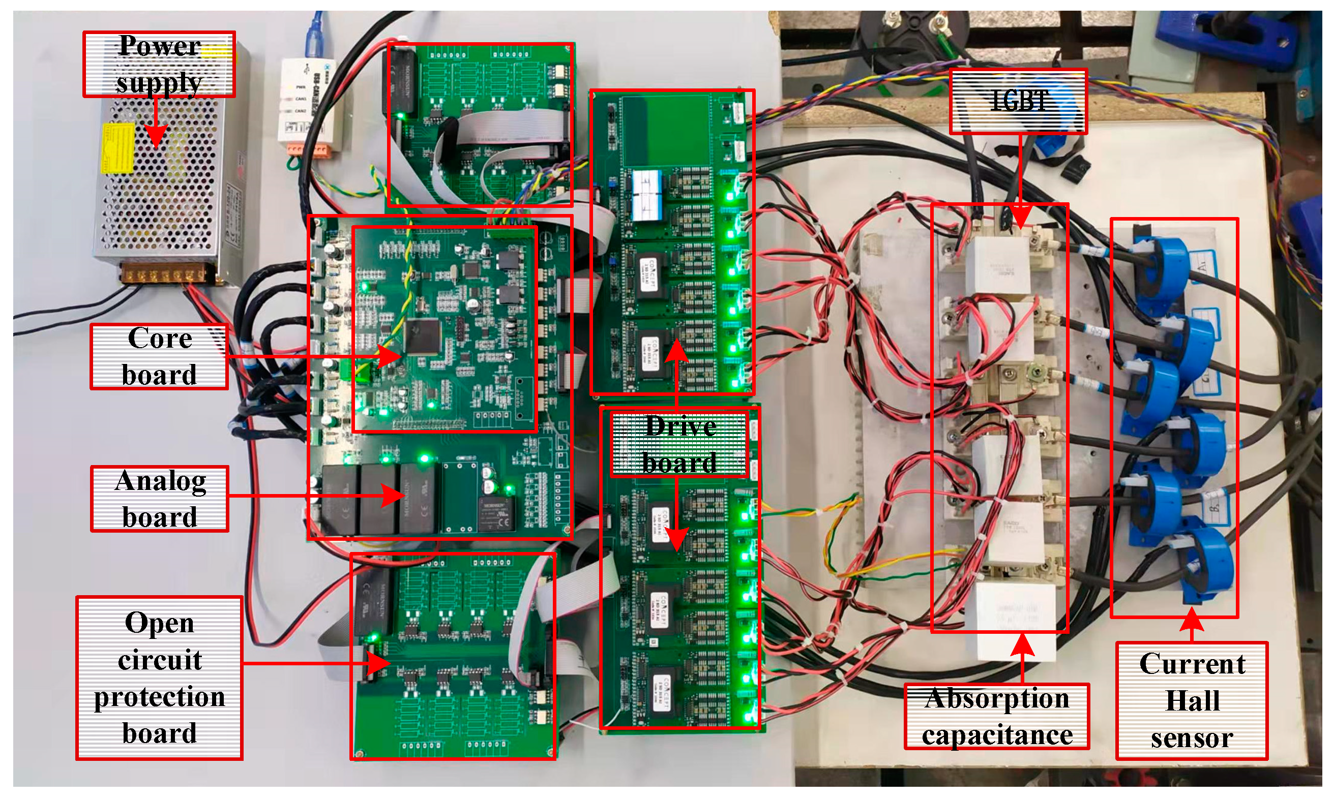
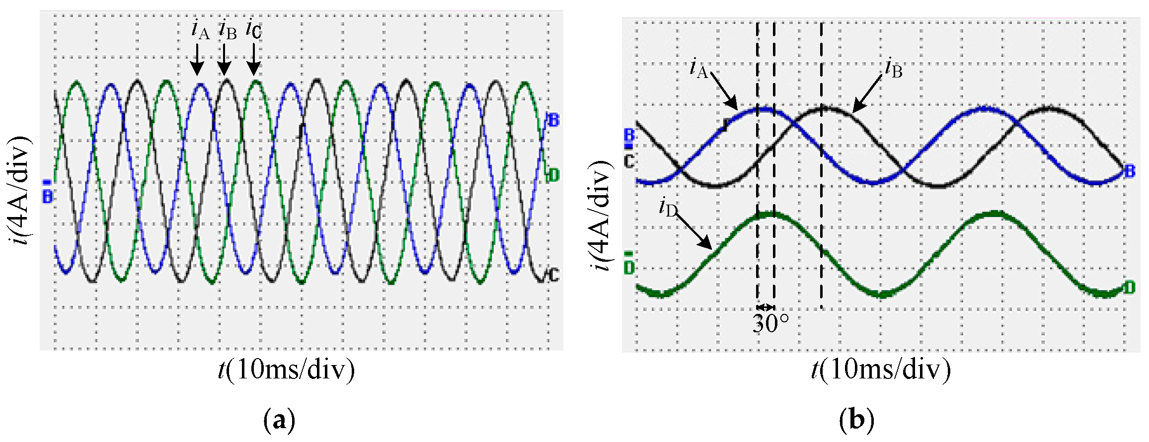
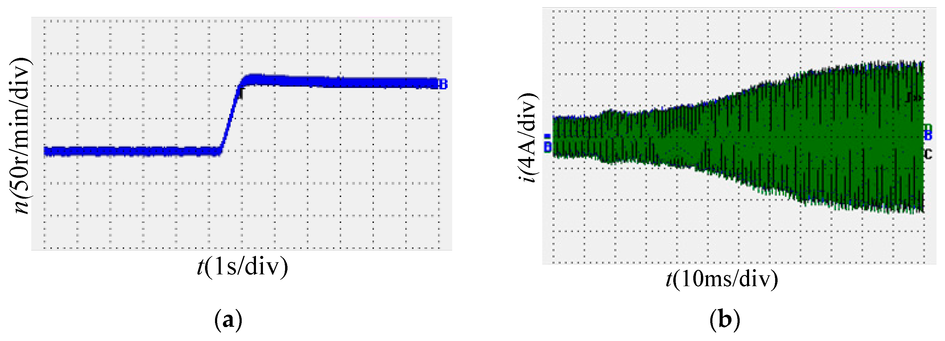
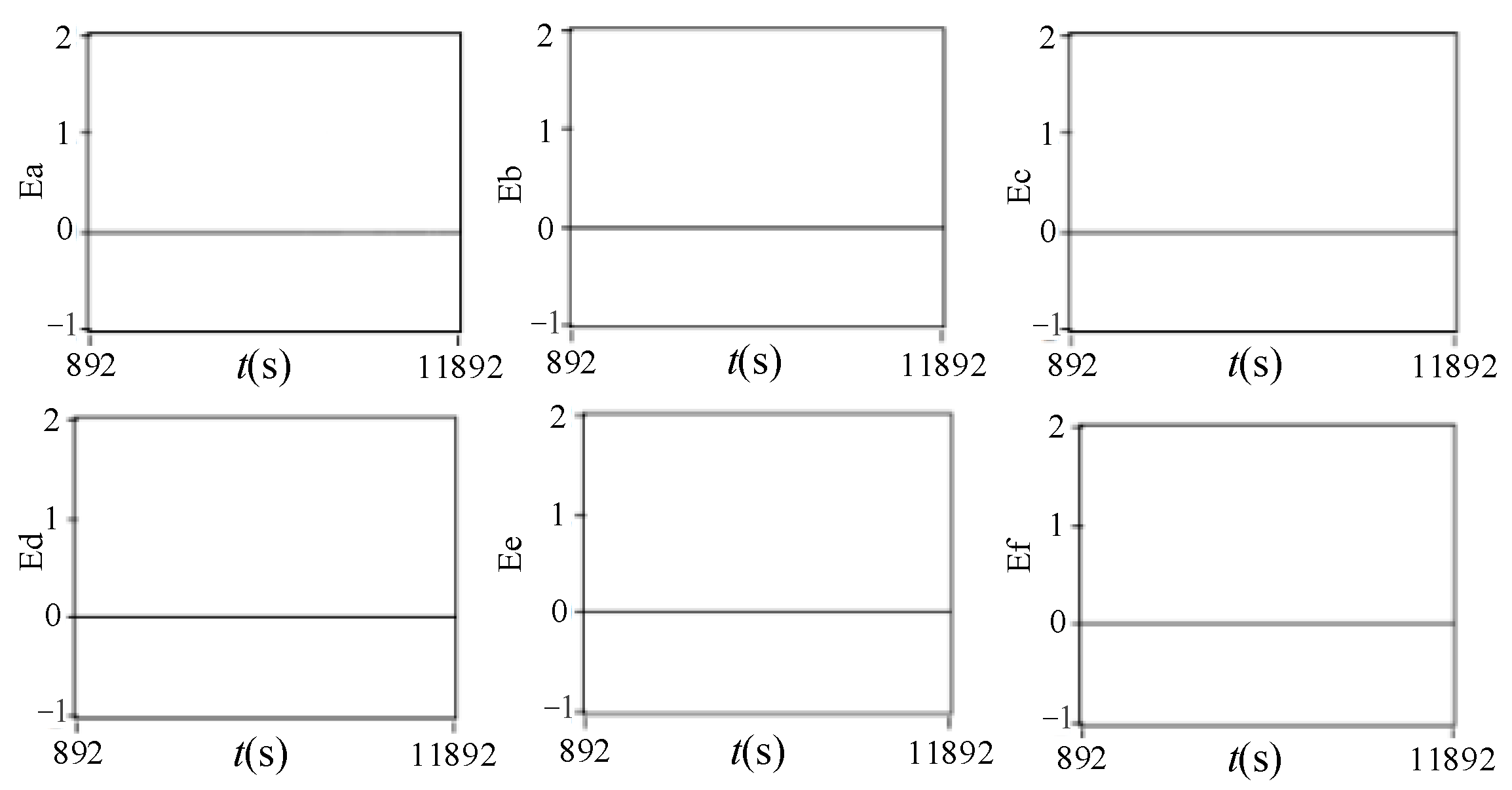
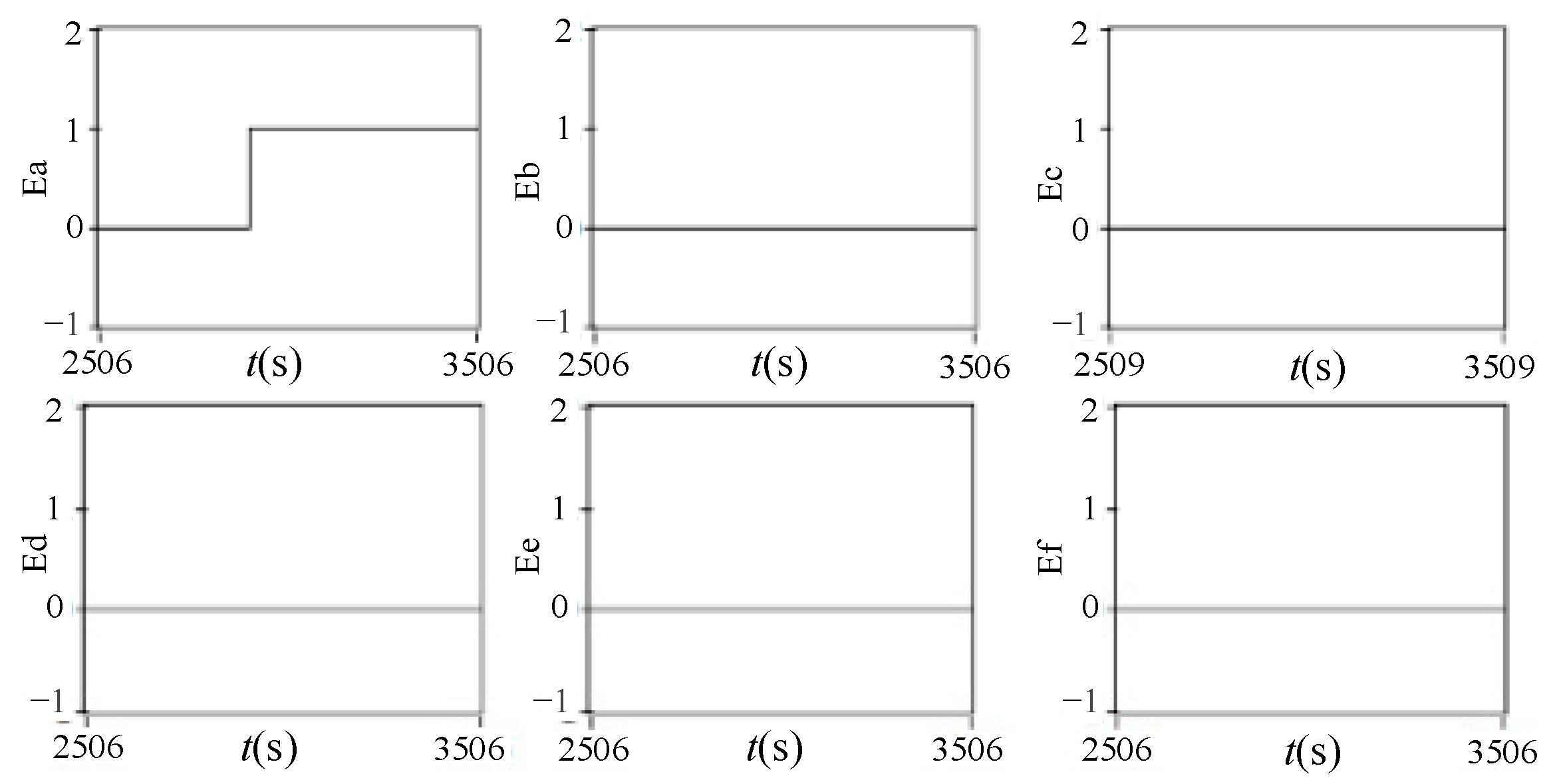
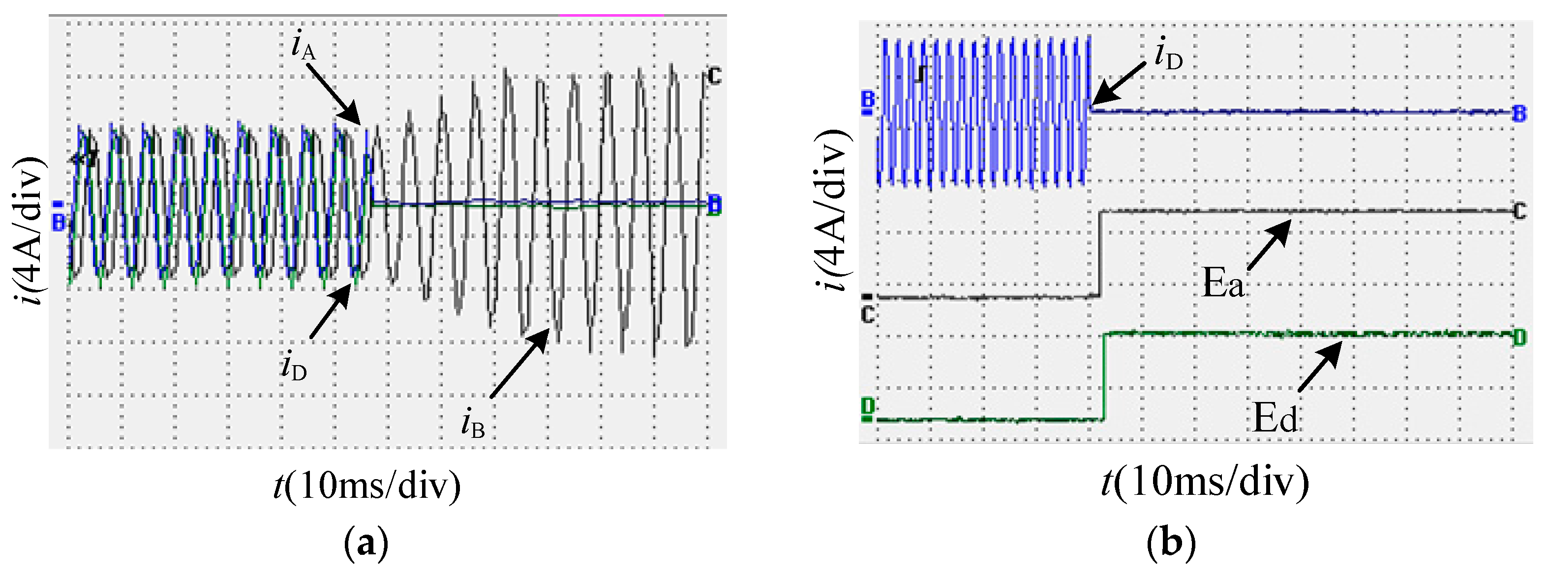
6. Experimental Verification

Figure 22 shows the overall block diagram of the six-phase PMSM control system, which provides the required DC bus voltage for the inverter after rectification by a three-phase uncontrolled rectifier bridge. The DSP-28335 chip outputs the IGBT driving waveform. The resolver and current hall sensor detect the position and phase current of the motor rotor. The Labview host computer platform can receive the motor running state and fault index waveform in DSP in real time.

In order to verify the proposed fault diagnosis algorithm, a six-phase motor experimental platform based on DSP is built. The experimental platform is shown in Figure 23. It is mainly composed of a rectifier, controller, inverter, and motor. The motor parameters are: rated output power P = 10 kW, rated voltage U = 311 V, rated current I = 20 A, rated speed N = 1500 r/min, rated torque T = 60 N·m, pole pair p = 5, quadrature axis and straight axis inductor L_d = L_q = 8.5 mH, and power factor = 0.94.

Figure 24 shows the phase current waveform when the motor is running at 500 r/min. The current is observed by collecting the voltage at the two ends of the sampling resistance. The voltage value is 100 mV, which corresponds to a current value of 2 A. The amplitudes of the phase currents are equal with a high sinusoidal degree. The current waveforms of phase a, b, and d under the same conditions are shown in Figure 24a. The phase difference between phase d current and phase a current is 30 degrees. The waveform of the motor is smooth and sinusoidal during normal operation.

Figure 25 shows the motor speed and six-phase current waveform under sudden load. When the motor speed increases from 400 r/min to 500 r/min in Figure 25a, the actual motor speed gradually increases in the form of the slope with the given speed; the transition is gentle and the overshoot is small in the process of speed increase. In Figure 25b, the amplitude of the motor phase current gradually increases during loading, and the dynamic adjustment process is smooth and stable.

Figure 26 shows the motor speed and the six-phase current waveform during sudden load reduction. When the motor decelerates from 500 r/min to 400 r/min in Figure 26a, the actual motor speed gradually decreases in the form of the slope with the given speed. The transition is smooth and the overshoot is small during deceleration. In Figure 26b, the amplitude of the motor phase current gradually decreases during load reduction, and the dynamic regulation process is smooth and stable.

Figure 27 shows the fault index waveform of the motor during stable operation and sudden load increase and decrease. During stable operation and sudden load increase and decrease in the motor, the values of the six-phase open phase fault index are zero, and there is no change. The fault index has no misdiagnosis under fault-free operation, which proves that it has good robustness.

Figure 28 presents the phase current and fault index waveform of motor phase a in the case of phase failure. Figure 28a presents the current waveform before and after the fault, in which the blue, black, and green lines respectively represent the current waveform of phase a, b, and c of the motor. After the phase failure of phase a, the current value of this phase drops to zero, the current amplitude of phase b and c becomes almost twice the original one, and the phase positions are complementary. Figure 28b illustrates the waveform of the fault phase current and fault index. After the phase failure of phase a, the phase failure index Ea of phase a increases to a high level after 32 ms, and the optimized fault index has no obvious burr and peak pulse. Therefore, the fault diagnosis and early warning can be performed in a short time.

Figure 29 shows the fault index waveform of the six-phase disconnection when the a phase disconnection fault occurs. After the fault occurs, only the fault index Ea of phase a rises to 1, while the fault indexes of the other phases do not change, and there is no misdiagnosis.

The phase current and fault index waveform of phase a and phase d of the motor with phase failure, are shown in Figure 30. The blue, black, and green lines shown in Figure 30a represent the current waveforms of motor phases a, b, and d, respectively. After the phase failure of phase a and d, the corresponding phase current value drops to zero, and the amplitude of the phase b current increases. The six-phase failure index waveform of phase a and phase d is shown in Figure 31. Before the phase failure occurs, the six-phase failure index remains null. After the failure occurs, the failure indexes Ea and Ed of phase a and phase d rise to 1, while the other four-phase failure indexes remain null without misdiagnosis.

Figure 32 shows the phase current and fault index waveform of phase failure of phase a and phase f. The blue, black, and green lines shown in Figure 32a represent the current waveforms of motor phases a, b, and f, respectively. A phase failure occurs in phase a and phase f, and the current value drops to zero. After the failure of phase a and phase f, their failure indexes Ea and Ef jump to the high level after 22 ms and 24 ms, respectively. These situations show that the proposed open phase fault diagnosis method has a high diagnosis speed, and can accurately locate the fault phase position.

The six-phase failure index waveform of phase a and phase f is shown in Figure 33. During normal operation, the failure indexes of the two phases are 0. After phase a and phase f fail, their failure indexes Ea and Ef rise to 1, and the failure indexes of the other phases do not change. It can then be deduced that the fault index of each phase can accurately locate the position of the fault phase. In addition, the diagnosis results are accurate, and there will be no false diagnosis. Finally, the experimental results are coherent with the theoretical analysis, which verifies the correctness and efficiency of the proposed diagnosis algorithm.

7. Conclusions

This paper proposed a fault diagnosis method based on vector space decoupling (VSD). The open phase fault index is derived according to the VSD inverse transformation and the current constraints after the fault. The fault index is optimized in order to prevent misdiagnosis and improve reliability. The diagnosis of a single-phase and double-phase fault can be performed in one fundamental cycle. In addition, by considering the unique harmonic plane current track after VSD transformation as the characteristic signal, a neural network is used to identify different fault current tracks, in order to diagnose the switch fault. The simulation and experimental results show that the proposed scheme has a high detection speed, ability to deal with several fault types, and good robustness. Finally, the proposed approach can accurately locate the winding open-circuit fault and power switch fault, which can be used for inverter open-circuit fault diagnosis and provides a basis for maintenance personnel.

References

1. Boglietti, A.; Cavagnino, A.; Tenconi, A.; Vaschetto, S. The Safety Critical Electric Machines and Drives in the more Electric Aircraft: A survey. In Proceedings of the 2009 35th Annual Conference of IEEE Industrial Electronics, Porto, Portugal, 3–5 November 2009; pp. 2587–2594. [Google Scholar]
2. Ma, W.M.; Wang, D.; Cheng, S.W.; Chen, J.Q. Common basic scientific problems and technological development frontier of high performance motor system. Chin. J. Electr. Eng. 2016, 36, 2025–2035. [Google Scholar]
3. Yan, M.; Ma, W.M.; Ou, Y.B.; Mang, M.Z.; Lu, L. Study on performance of dual nine phase energy storage motor system. Chin. J. Electr. Eng. 2015, 35, 6. [Google Scholar]
4. Jeong, Y.S.; Sul, S.K.; Schulz, S.E.; Patel, N.R. Fault Detection and Dault Tolerant Control of Interior Permanent Magnet Motor Drive System for Electric Vehicle. IEEE Trans. Ind. Appl. 2003, 41, 1458–1463. [Google Scholar]
5. IEEE Committee Report. Report of Large Motor Reliability Survey of Industrial and Commercial Installations. IEEE Trans. Ind. Appl. 1985, 23, 153–158. [Google Scholar]
6. Gao, H.W.; Su, J.Y.; Yang, G.J. Open circuit fault diagnosis method of five phase inverter based on pole voltage error standardization. Chin. J. Electr. Eng. 2016, 36, 10. [Google Scholar]
7. Zhang, Z.; Luo, G.A. Hybrid Diagnosis Method for Inverter Open-Circuit Faults in PMSM Drives. China Electrotech. Soc. Trans. Electr. Mach. Syst. 2020, 4, 180–189. [Google Scholar] [CrossRef]
8. Diallo, D.; Benbouzid, M.E.H.; Hamad, D.; Pierre, X. Fault Detection and Diagnosis in an Induction Machine Drive: A Pattern Recognition Approach Based on Concordia Stator Mean Current Vector. IEEE Trans. Energy Convers. 2005, 20, 512–519. [Google Scholar] [CrossRef] [Green Version]
9. Yang, Z.L.; Wu, Z.G.; Li, H. Open circuit fault diagnosis method of inverter based on DC side current detection. Chin. J. Electr. Eng. 2008, 28, 18–22. [Google Scholar]
10. Dabour, S.M.; Rashad, E.; Hammad, R. Open-Circuit Fault Detection of Asymmetrical Six-phase Induction Motor Fed from Z-Source Inverter. In Proceedings of the 2019 21st International Middle East Power Systems Conference (MEPCON), Cairo, Egypt, 17–19 December 2019; pp. 1216–1222. [Google Scholar]
11. Zhang, Z.; Qi, S.; Liu, X. A Diagnosis Method for Open Circuit Fault of Dual Three-Phase Permanent Magnet Synchronous Motor Drive System. In Proceedings of the 2018 21st International Conference on Electrical Machines and Systems (ICEMS), Jeju, Korea, 7–10 October 2018; pp. 1425–1430. [Google Scholar]
12. Yang, C.; Gui, W.; Chen, Z.; Zhang, J.; Peng, T.; Yang, C. Voltage Difference Residual-Based Open-Circuit Fault Diagnosis Approach for Three-Level Converters in Electric Traction Systems. IEEE Trans. Power Electron. 2019, 35, 3012–3028. [Google Scholar] [CrossRef]
13. Chen, Y.; Zhang, J.J.; Chen, Z.Y. On line diagnosis of open circuit fault of three-phase inverter circuit based on current observer. J. Electrotech. 2019, 34, 609–617. [Google Scholar]
14. Chen, C.B.; Wang, X.X.; Gao, S.; Zhang, Y.M. Open circuit fault diagnosis method of inverter based on interval sliding mode observer. Chin. J. Electr. Eng. 2020, 40, 4569–4579. [Google Scholar]
15. Danjiang, C.; Yinzhong, Y. Open circuit fault diagnosis method of three-level inverter based on multi neural network. J. Electrotech. 2013, 28, 120–126. [Google Scholar]
16. Cai, F.Y. Research on Fault Diagnosis and Fault Tolerant Operation of Underwater Permanent Magnet Synchronous Motor Driver; Harbin Institute of Technology: Harbin, China, 2016. [Google Scholar]
17. Zhang, X.D.; Xu, B.J.; Wu, G.X.; Zuo, Y.B. Research on wind turbine fault diagnosis expert system. Manuf. Autom. 2014, 36, 21–25. [Google Scholar]
18. Trabelsi, M.; Nguyen, N.K.; Semail, E. Real-Time Switches Fault Diagnosis Based on Typical Operating Characteristics of Five-Phase Permanent Magnetic Synchronous Machines. IEEE Trans. Ind. Electron. 2016, 63, 4683–4694. [Google Scholar] [CrossRef] [Green Version]
19. Zhou, C.Y.; Shen, Y.X. Open circuit fault diagnosis of double three-phase voltage source inverter based on wavelet analysis. J. Mot. Control. 2020, 24, 65–75. [Google Scholar]
20. Chen, Y.; Liu, Z.L.; Chen, Z.Y. Fast diagnosis and location method of inverter open circuit fault based on current vector feature analysis. J. Electrotech. 2018, 33, 883–891. [Google Scholar]
21. Cui, J.; Wang, Q.; Gong, C.Y. Research on inverter power tube fault diagnosis technology combined with wavelet and Concordia transform. Chin. J. Electr. Eng. 2015, 35, 3110–3116. [Google Scholar]
22. Hu, Y.; Li, Y.; Ma, X.; Li, X.; Huang, S. Flux-Weakening Control of Dual Three-Phase PMSM Based on Vector Space Decomposition Control. IEEE Trans. Power Electron. 2021, 36, 8428–8438. [Google Scholar] [CrossRef]
23. Xie, R.; Wang, X.M.; Li, Y.; Zhao, K.R. Research and application on improved BP neural network algorithm. In Proceedings of the 2010 5th IEEE Conference on Industrial Electronics and Applications, Taichung, Taiwan, 15–17 June 2010; pp. 1462–1466. [Google Scholar]
24. Cheng, H.; Cui, L.; Li, J. Application of improved BP neural network based on LM algorithm in desulfurization system of thermal power plant. In Proceedings of the 2017 Chinese Automation Congress (CAC), Jinan, China, 20–22 October 2017; pp. 5917–5920. [Google Scholar]
Figure 1. Topology of the six-phase inverter with neutral isolation.
Electronics 11 01229 g001
Figure 2. α-β and z1-z2 plane current waveform during normal operation: (a) α-β plane current waveform in case of normal operation; (b) z1-z2 plane current waveform in case of normal operation.
Electronics 11 01229 g002
Figure 3. Fault index optimization process of disconnected phase.
Electronics 11 01229 g003
Figure 4. z1-z2 plane current in case of different power switch faults; (a) z1-z2 plane current waveform in case of T1 fault; (b) z1-z2 plane current waveform in case of T1 and T2 faults.
Electronics 11 01229 g004
Figure 5. Reference direction of iz1 and iz2 current trace in the case of a single switch failure.
Electronics 11 01229 g005
Figure 6. Reference direction of iz1 and iz2 current trace, in the case of two-power-switch faults.
Electronics 11 01229 g006
Figure 7. Single neuron structure.
Electronics 11 01229 g007
Figure 8. Neural network structure model.
Electronics 11 01229 g008
Figure 9. Current waveform of load and disturbance during normal operation.
Electronics 11 01229 g009
Figure 10. Fault indicators under normal operation load and disturbance.
Electronics 11 01229 g010
Figure 11. Phase a current waveform of open-circuit fault in 0.3 s.
Electronics 11 01229 g011
Figure 12. Phase a fault indicator waveform when open fault occurs within 0.3 s.
Electronics 11 01229 g012
Figure 13. Current waveforms of phase a and phase d at 0.3 s and 0.5 s open-circuit fault, respectively.
Electronics 11 01229 g013
Figure 14. Fault index waveforms of phase a and phase d at 0.3 s and 0.5 s open-circuit fault, respectively.
Electronics 11 01229 g014
Figure 15. Current waveforms of phase a and phase f at 0.3 s and 0.5 s open-circuit fault, respectively.
Electronics 11 01229 g015
Figure 16. Fault index waveforms of phase a and phase f at 0.3 s and 0.5 s open-circuit fault, respectively.
Electronics 11 01229 g016
Figure 17. z1-z2 harmonic plane current trace in case of single-switch fault.
Electronics 11 01229 g017
Figure 18. z1-z2 harmonic plane current trace in case of two-switch fault.
Electronics 11 01229 g018
Figure 19. Neural network training model.
Electronics 11 01229 g019
Figure 20. Error convergence curve of neural network.
Electronics 11 01229 g020
Figure 21. Regression curve of neural network training error.
Electronics 11 01229 g021
Figure 22. Overall block diagram of the six-phase PMSM control system.
Electronics 11 01229 g022
Figure 23. Experimental platform of the six-phase motor control system.
Electronics 11 01229 g023
Figure 24. Waveform of motor under stable operation at 500 r/min: (a) current waveform of phase a, b, and c; (b) current waveform of phase a, b, and d.
Electronics 11 01229 g024
Figure 25. Waveform of the motor under sudden load: (a) speed waveform; (b) current waveform of the six-phase motor.
Electronics 11 01229 g025
Figure 26. Waveform of the motor under sudden load: (a) speed waveform; (b) current waveform of the six-phase motor.
Electronics 11 01229 g026
Figure 27. Fault index waveform under stable operation at 500 r/min.
Electronics 11 01229 g027
Figure 28. Phase current and fault index waveform in case of phase failure of phase a: (a) fault current waveform; (b) fault phase current and fault index waveform.
Electronics 11 01229 g028
Figure 29. Fault index waveform in case of phase failure of phase a.
Electronics 11 01229 g029
Figure 30. Phase current and fault index waveform in case of phase failure of phase a and phase d: (a) fault current waveform; (b) fault phase current and fault index waveform.
Electronics 11 01229 g030
Figure 31. Fault index waveform in case of phase failure of phase a and phase d.
Electronics 11 01229 g031
Figure 32. Phase current and fault index waveform in case of phase failure of phase a and phase f: (a) fault current waveform; (b) fault phase current and fault index waveform.
Electronics 11 01229 g032
Figure 33. Fault index waveform in case of phase failure of phase a and phase f.
Electronics 11 01229 g033