Machine-Learning-Based Uplink Throughput Prediction from Physical Layer Measurements

Abstract

The uplink (UL) throughput prediction is indispensable for a sustainable and reliable cellular network due to the enormous amounts of mobile data used by interconnecting devices, cloud services, and social media. Therefore, network service providers implement highly complex mobile network systems with a large number of parameters and feature add-ons. In addition to the increased complexity, old-fashioned methods have become insufficient for network management, requiring an autonomous calibration to minimize utilization of the system parameter and the processing time. Many machine learning algorithms utilize the Long-Term Evolution (LTE) parameters for channel throughput prediction, mainly in favor of downlink (DL). However, these algorithms have not achieved the desired results because UL traffic prediction has become more critical due to the channel asymmetry in favor of DL throughput closing rapidly. The environment (urban, suburban, rural areas) affect should also be taken into account to improve the accuracy of the machine learning algorithm. Thus, in this research, we propose a machine learning-based UL data rate prediction solution by comparing several machine learning algorithms for three locations (Houston, Texas, Melbourne, Florida, and Batman, Turkey) and determine the best accuracy among all. We first performed an extensive LTE data collection in proposed locations and determined the LTE lower layer parameters correlated with UL throughput. The selected LTE parameters, which are highly correlated with UL throughput (RSRP, RSRQ, and SNR), are trained in five different learning algorithms for estimating UL data rates. The results show that decision tree and k-nearest neighbor algorithms outperform the other algorithms at throughput estimation. The prediction accuracy with the R2 determination coefficient of 92%, 85%, and 69% is obtained from Melbourne, Florida, Batman, Turkey, and Houston, Texas, respectively.

1. Introduction

Broadband data usage is facing a massive demand with the availability of the fourth-generation (4G) and evolving fifth-generation (5G) wireless technology. These technologies promise higher spectral efficiency, low latency, high peak data rates, and flexibility in frequency and bandwidth to the end-user [1]. Hence, it is crucial to maintain the Quality of Service (QoS), while guaranteeing reliable and robust networks with achieving higher data rates. In wireless communications, data rates have increased exponentially from second generation (2G/GSM) (data speed up to 9.6 Kbps) to 4G/LTE (data speed up to 300 Mbps). LTE employs 20 MHz bandwidth with different modulation and multiplexing techniques such as Orthogonal Frequency Division Multiple Access (OFDM), 64 QAM, and 4 × 4 spatial multiplexing to achieve higher data rates [2,3]. Higher-resolution video and audio content have become widespread with reliable and fast mobile internet access. The demand for cellular data doubles every two years and is expected to reach 77.5 exabytes by 2022 [4]. Under the umbrella of the Internet of Things (IoT), massive mobile applications at an unprecedented pace lead to reliable networks and higher peak data rates. In November 2019, COVID-19 was identified in Wuhan, China, and became a pandemic in a short time. Online education, working from home, and online businesses have become widespread as the world has experienced lockdowns due to the pandemic. This new normal has led the world to comprehend the necessity of UL throughput and innovative cellular technologies eminently. According to Lutu et al., pandemics such as the SARS-CoV-2 virus can drastically impact the network data traffic in favor of UL demand. Their results confirm an increase of 10% in UL mobile data usage and a decrease of 20% in DL mobile data usage [5].

As stated by cellular standards, the DL contains more measurement elements and traceable features than the UL [6]. Naturally, carriers tend to focus more on the DL and deploy an asymmetric channel capacity between DL and UL channels [7]. Due to this asymmetric deployment, the DL channel has a higher transmission capacity than the UL. However, the need for UL data has increased considerably with the rapid increase in the use of applications that require UL throughput, such as AV control, machine type communication devices (MTDs) smart body area networks (SmartBAN), IoT, wireless sensor networks, video conferencing, file sharing, VoIP, surveillance cameras, peer-to-peer (P2P) and cloud services [8,9,10,11,12,13,14]. Although many studies have focused on DL channel prediction due to the much higher demand for DL data rate before, UL traffic estimation has gained significance since the channel asymmetry in favor of DL throughput is closing rapidly [15]. MTD applications that rely on vast amounts of small data packets transmitted via the UL channel can place extremely heavy congestion on the channel [16]. This congestion will cause significant difficulties for cellular networks, and if optimizations are not made, it becomes inevitable to use 5G network systems that occupy a large amount of traffic in the UL direction [17]. SmartBANs, which are networks of sensors embedded in the human body that provide beneficial health care monitoring such as EEG, EKG, blood pressure, etc., also mostly use UL transmission. Therefore, possible channel congestion may delay the vital feedback about the patient’s health [18]. Carson and Lundvall state that around 20% of end-users are dissatisfied with their UL data rate [19]. The complaints will require data collection and optimization of UL channels in cellular networks. However, the outdated rule-based techniques cannot bear even current system requirements due to the unprecedented growth of the number of parameters, carrier features, and counters. Machine learning (ML) algorithms used in the most complex tasks in every field [20] are great for designing and optimizing mobile networks.

ML’s primary concept is to create autonomous systems that learn from data throughput by identifying patterns and making decisions based on results [21]. The learning process and its implementation are illustrated in Figure 1.

There are several commonly used ML algorithms, such as decision trees, linear regression, artificial neural networks (ANN), and K-nearest neighbor. After calculating the cost, weights are adjusted through a gradient descent algorithm and repeated until gradient descent converges to the optimum value. This convergence is called “the learning process” and is valid for almost every machine learning algorithm.

Recently, 4G has become the dominant technology in cellular networks globally and soon will be introduced in leading radio mechanisms, 5G systems. While using these technologies, it is critical to provide a stable and high UL throughput in emergencies. For instance, it is essential to use AI-aided autonomous ambulance drones to speed up emergency responses, prevent deaths, and accelerate recovery dramatically [22]. Thus, a robust UL throughput predicting mechanism is required to ensure the highest quality of service.

LTE has various radio measurements that can be a key input for machine learning to model and predict UL throughput. Using ML algorithms, this research evaluates the lower layer LTE radio metrics for UL throughput prediction. This study utilizes three datasets collected from Melbourne, Florida, Houston, Texas, and Batman, Turkey. It is also one of the first in a series to initiate model development and create a framework from a comprehensive data set. The paper continues with the following sections: literature review, understanding of machine learning algorithms, data collection, and prediction results and analysis.

2. Literature Review

Minimizing the latency, geopositioning of systems, and keeping the throughput at a premium are necessary for modern telecommunication systems such as LTE and upcoming 5G technologies. As mobile applications need more content to be delivered wirelessly, e.g., video streaming and 3D point clouds, modeling and optimizing the throughput become indispensable in terms of QoS. Cellular mobile networks utilize throughput models that contain history-based, computational-based, and ML-based predictions for design and optimization. History-based predictions mainly extrapolate archived data, which contains various parameters, including time, place, and density of the traffic, to decide. On the other hand, computation-based predictions evaluate a mathematical model as a function of several variables to derive a decision. Nevertheless, there is still a lack of accuracy in both approaches, especially on the UL side.

An experiment conducted by Yue et al. benefits from stationary LTE measurements taken from regional routes, highways, and pedestrian lanes to forecast DL throughput. The study performs ML algorithms on two US cellular operators and achieves an error rate between 4 and 17% [23]. Even though the study has high accuracy in DL prediction, it still needs to be improved to eliminate error fluctuation. In his study, Jomrich et al. seek a reliable cellular data connection since mobility causes significant oscillation in QoS. Thus, they investigated an automated bandwidth prediction model aided by ML algorithms. They stated that their machine learning algorithms were lightly affected by additional oscillations caused by vehicle velocity [24]. Bojovic et al. researched the Self-Organizing Network (SON) to reduce the time and expenditure of the network processes. Learning-based SON uses key performance indicators (KPI’s) as estimation parameters and can adapt dynamically to the environment for QoS improvement purposes. The researchers used LTE parameters such as dynamic frequency and bandwidth assignment with 95% of optimal network performance [25]. Finally, Oussakel et al. investigated a machine learning solution to manage the immense demand for UL transmission to increase the QoS. As stated in their work, the main supervised learning algorithms are utilized to predict UL bandwidth in the range of 88% to 94% with different scenarios [26].

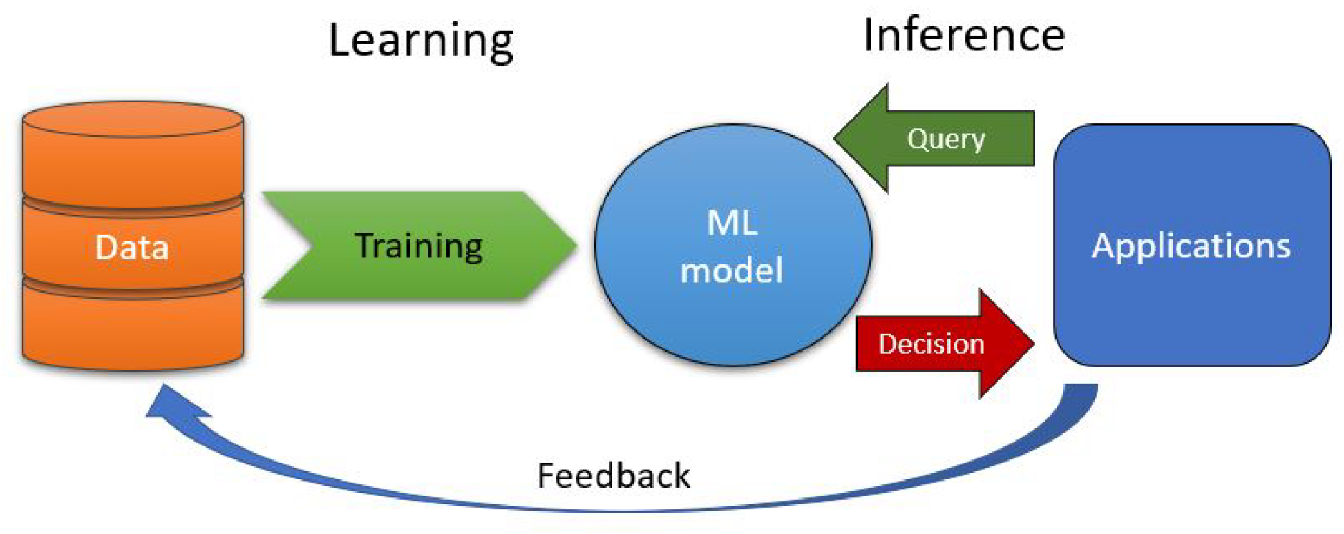
3. Understanding Machine Learning Algorithms

Machine learning evolved from the field of data analytics, including computational learning and pattern recognition. ML comprises many mathematical models to make predictions for specific tasks. Since it has a variety of applications such as e-mail filtering, anomaly detection, and image recognition, it is a popular tool for researchers, engineers, and data scientists [27,28,29]. This section will explain some of the important machine learning algorithms in detail.

3.1. Linear Regression

Linear regression is an ML algorithm that seeks a linear relationship between the number of independent variables ($\hat{x}$) and the dependent variable ($\widehat{y}$). The equation that is used to predict a linear regression line is indicated in Equation (1).

$${\widehat{y}}_i={\hat{\beta }}_0+{\hat{\beta }}_1{x}_i+{\widehat{ϵ}}_i$$

(1)

The intuition behind the linear regression algorithm is to determine the best values for coefficients ${\hat{\beta }}_0$ and ${\hat{\beta }}_1$. Cost function and slope are essential key concepts to derive results for coefficients ${\hat{\beta }}_0$ and ${\hat{\beta }}_1$. Equation (2) represents the cost function and investigates the minimum value of the cost function.

$$minimize\left(\frac{1}{n}\sum _{i=1}^n{(y_i-\overline{y})}^2\right)$$

(2)

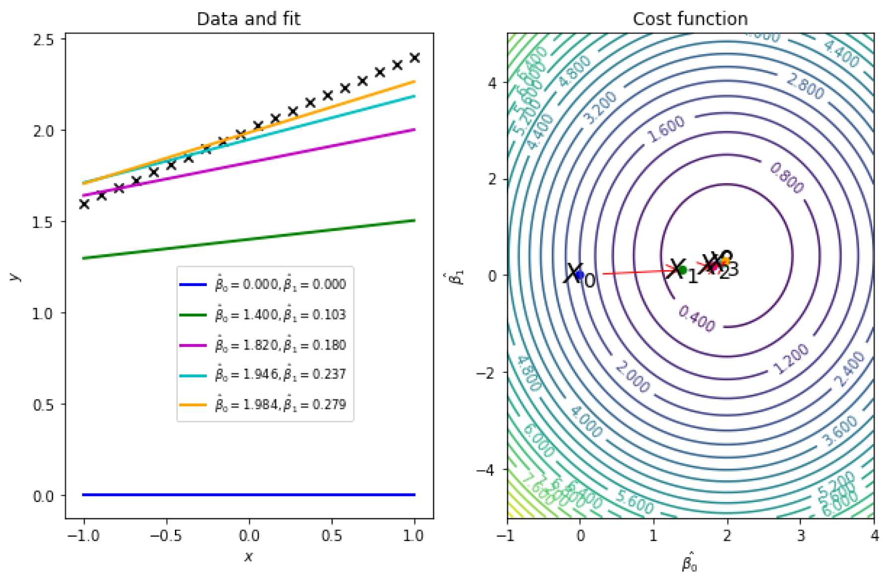
3.2. Gradient Descent

Gradient descent is one of the first-order methods which basically begin with an initial point and repeatedly move its steps in the direction of the gradient descent that minimize the $f\left(x\right)$ function as seen in Algorithm 1 [30]:

Algorithm 1 The Gradient Descent Algorithm

for $k=0,1,2,\dots$ do    $g_k\leftarrow \nabla f\left(x_k\right)$    $x_{k+1}\leftarrow x_k-t_k{g}_k$  end for

Where k is the number of iterations, $g_k$ is the gradient of the dependent variable, and $x_k$ is the independent variable. The gradient descent iterative action is shown in Figure 2. According to Equation (1), there are two coefficients as ${\hat{\beta }}_0$ and ${\hat{\beta }}_1$ presented as contour levels. The starting point of gradient descent, $x_0$, moves to $x_1$, then from $x_1$ to $x_2$, until it converges to the optimum value. The ideal optimum value is the middle of the circles, which indicates the global minimum. Figure 3 also shows the local minimum, which may cause deceptive predictions. Gradient descent does an iterative update to find the best coefficients leading the global minimum.

By definition, the gradient descent algorithm has several criteria to find its direction during the iterative process, such as the initial point $x_0$, step size $t_k$, and stopping condition. Since these criteria are linked to each other, a wrong choice may end up with a local minimum instead of the global minimum. Besides, the technique called early stopping, a form of regularization, should be applied to a gradient descent algorithm to avoid the over-fitting problem. However, implementing such techniques increases the learning performance with each iteration, which leads to a higher generalization error. Thus, it is wise to skip the early stopping and keep $f\left(x_k\right)$ as close as possible to the global minimum. The following convergence bounds rule should be applied to determine the minimum number of steps:

$$k\ge k_f(f\left(x_0\right)-f\left(x^{*}\right))g\left(\frac{1}{\epsilon }\right)$$

(3)

where k is the number of iterations, $k_f$ is a feature estimated from the independent variables of the function, g is a function dependent on the independent variable of the function, $\epsilon$ is the error of confidence, and $f\left(x^{*}\right)$ is the true minimum.

3.3. Gradient Boosting Regression

Boosting is a technique that is applied to base learners of machine learning tools such as regression and classification. Boosting is a doping factor for poor iterative models and a way to combine multiple weak models into one single model. Different boosting techniques reveal the quantity of the misclassification and pick the appropriate option for the next iteration. This mainly decreases the bias due to the focus on misclassified cases. In this research, we employ Gradient Boosting Regression (GBR) as a boosting technique.

The GBR uses gradient terms for prediction since it utilizes the gradient descent algorithm to minimize the cost function. Even though there is a slight difference between The GBR and linear regression, GBR has a notable increase in accuracy. The GBR is generally used with decision trees (DT) of fixed-size base learners. The GBR determines the error between the current prediction and actual values. This error is called residual. The GBR trains weak models, which maps features to this residual. After acquiring the residual, it combines them with the input of the existing model. This iterative process pushes the model in the direction of the actual value and improves the overall model prediction [31]. The GBR is represented in Algorithm 2.

Algorithm 2 The GBR Algorithm

1. Initialize model with a constant value: $$F_0\left(x\right)=argmin\sum _{i=1}^{n}Loss(y_i,\gamma )$$ (4) 2. i=1:M 1. Compute the so-called pseudo-residuals: $$r_{im}=-{\left[\frac{\partial Loss(y_i,F\left(x_i\right))}{\partial F\left(x_i\right)}\right]}_{F\left(x\right)=F_{m-1}\left(x\right)}\mathrm{for} i=1,\dots ,n.$$ (5) 3. Fit a weak learner $h_m\left(x\right)$ to pseudo-residuals, i.e., train it using the training set ${\left\{(x_i,r_{im})\right\}}_{i=1}^n$ 4. Compute multiplier ${\gamma }_m$ by solving the following one-dimensional optimization problem: $${\gamma }_m=\underset{\gamma }{arg\; min}\sum _{i=1}^{n}Loss\left(y_i,F_{m-1}\left(x_i\right)+\gamma h_m\left(x_i\right)\right)$$ (6) 5. Update the model: $$F_m\left(x\right)=F_{m-1}\left(x\right)+{\gamma }_m{h}_m\left(x\right)$$ (7) 6. Output $F_M\left(x\right)$ where $F_0\left(x\right)$ is an intended function. $\gamma$ represents the learning rate.

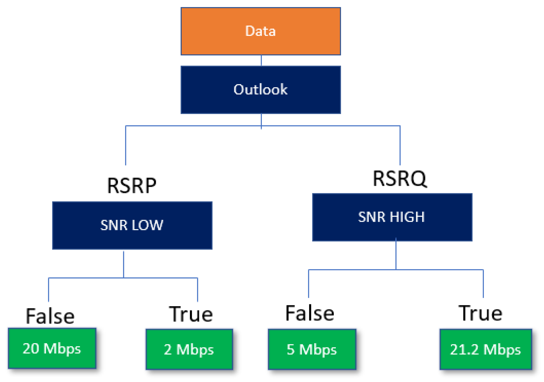
3.4. Decision Tree Regression (DTR)

DTR is a prediction model based on recursive partitioning of features into a tree-like structure. It is like a hierarchical flowchart with internal nodes, and every node has an attribute to test and classify an outcome. Based on probability, the nodes are assigned to a related class. Thus, even slight variations may end up with different DTs [32]. Figure 3 shows a flowchart representation of DTs. According to the flowchart, the data stream goes through the outlook and checks the RSRP and RSRQ classes. If the class comprises low SNR, then it picks RSRP, else, it picks RSRQ. If RSRP and RSRQ branches determine the throughput under or over the predefined threshold, then it makes a decision accordingly.

3.5. K-Nearest Neighbors (KNN)

The KNN algorithm is a supervised learning algorithm meant to solve classification, pattern recognition, and regression problems. It is also a non-parametric technique that can be used in various applications. The KNN algorithm considers that similar attributes should be close to the selected data points [33]. K demonstrates the number of nearest neighbors, which is crucial for prediction accuracy. The distance vectors ($D_{KNN}(x_i,y_i)$) are generally determined by Manhattan distance formula as seen in Equation (8) [34].

$$D_{KNN}(x,y)=\sum _{i=1}^n\mid x_i-y_i\mid$$

(8)

Root Mean Square Prediction Error (RMSPE) is used with a cross-validation method to choose the best k number. Then, the target prediction is made by taking the average of k nearest data points. The mathematical formula of RMSPE is indicated in Equation (9) [35].

$$RMSPE=\sqrt{\frac{1}{n}\sum _{i=1}^n{(y_i-{\widehat{y}}_i)}^2}$$

(9)

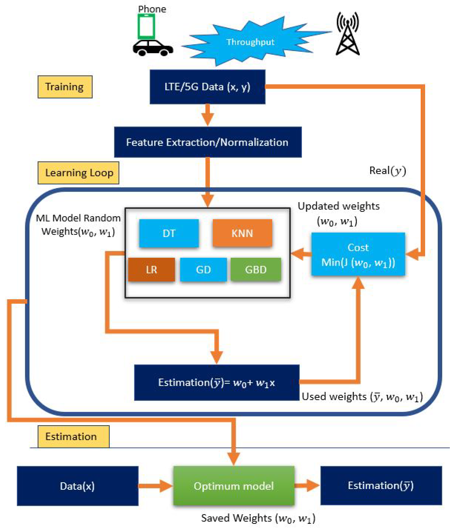
4. Modeling Uplink Throughput Prediction

This section describes the stages of UL throughput prediction via commonly used machine learning algorithms, as illustrated in Figure 4. The LTE data set is collected through a driving test and a phone mounted on the car in the initial process. Due to the noise and environment, the collected LTE data set contains non-numerical values and repetitions, impacting the ML analysis in the feature extraction/normalization phase. Therefore, these faulty values should be cleaned out from the data before the feature extraction phase. After cleaning the faulty values, correlation analysis between UL throughput and lower-layer LTE parameters. Finally, target parameters that show a higher correlation with UL throughput (RSRP, RSRQ, and SNR) are transferred to the learning loops of five commonly used ML algorithms. In this phase, also called training, each ML algorithm builds its estimation model. In each loop, the provisional prediction results are compared to actual UL throughput values to obtain errors called the cost or entropy. These cost functions adjust the models towards the optimum values until the stopping criteria are fulfilled. This section will evaluate the five ML algorithms’ analyses and their UL throughput outcomes.

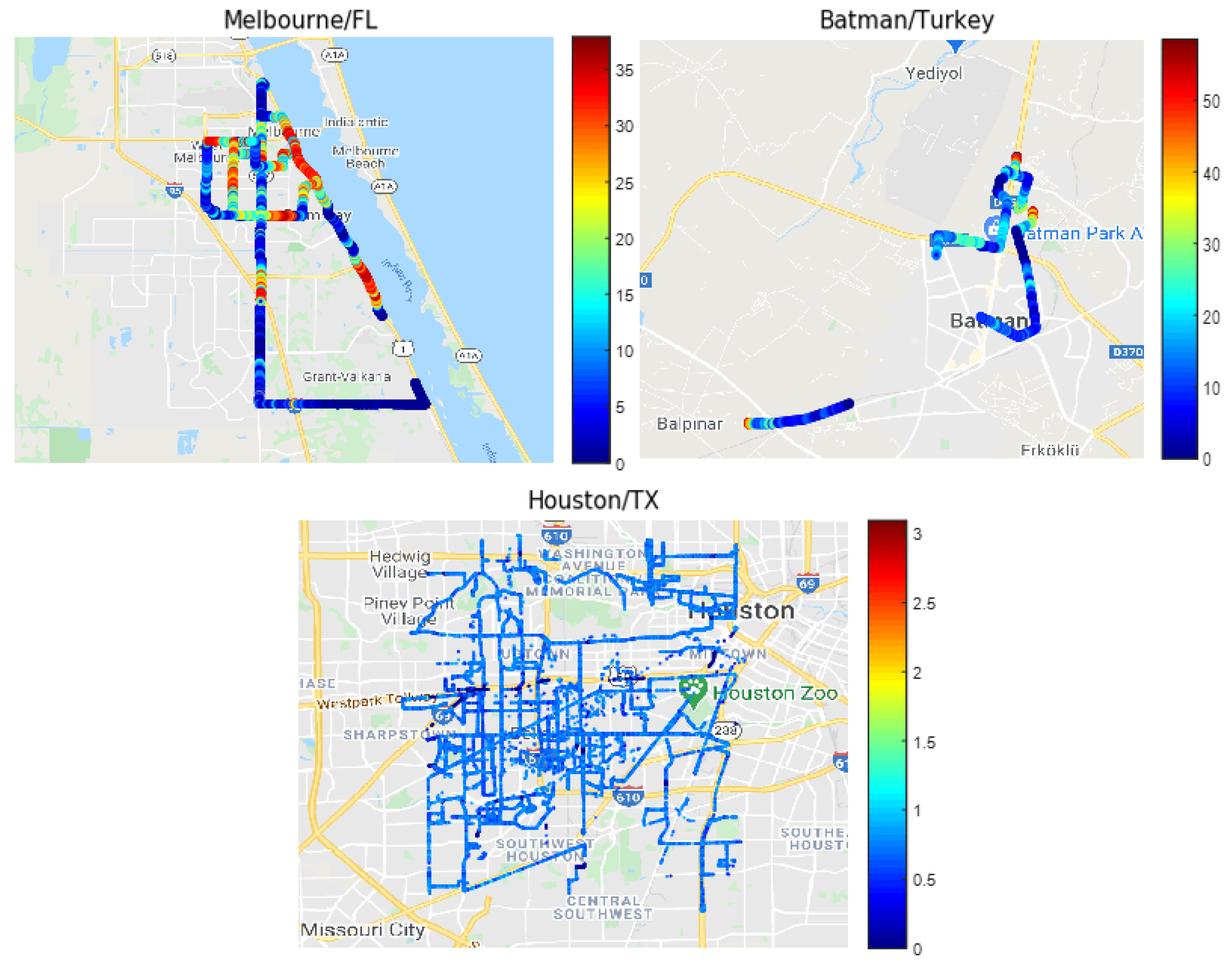
4.1. Data Collection

Three data sets from different locations (Melbourne, Florida, Batman, Turkey, Houston, Texas) with varying natural characteristics were collected and tested to validate this endeavor’s accuracy. Geographical visualization of the data sets is illustrated in Figure 5 with the UL throughput heat maps. Melbourne and Batman data sets were collected under similar and stable weather conditions and with the same UE velocity. However, we do not know under what conditions the Houston data set was collected since one of the major US cellular companies provided these data. The first test data were collected from the Melbourne, FL, area with suburban nature characteristics. RantCell Test Analytics measurement application is installed on a Samsung Note 10 (SM-N9750/u) smartphone, and all tests were conducted with that device in this area. The data collection part took ten days (from 14 to 25 September) under mostly similar weather conditions. The weekdays at different periods were chosen for receiving realistic results. The data collection was performed in the same paths each day to reduce the number of active users’ effect on UL data rates. The average car speed was 40 mph, and the testing and equipment configuration was frequently checked. We followed the same configurations and procedures in the second data collection. The second data set was gathered from Batman, Turkey, which has an urban nature characteristic from 5 to 16 October. A cellular network company provided the last data set collected in Houston, Texas, where metropolitan nature characteristics dominate. The operator data were collected between 31 March and 13 April. The following key performance parameters were trained in the machine learning algorithms to predict UL throughput prediction:

• RSRP (reference signal received power) is the average power of cell-specific signals in the channel bandwidth. RSRP is used for cell selection and coverage since it has signal strength information. The range of RSRP values is between −140 dBm and −44 dBm;
• RSRQ (received signal received quality) indicates the quality of the signal;
• SNR (signal-to-noise ratio) is used directly in the modulation and coding scheme to select one in 77 modulation schemes.

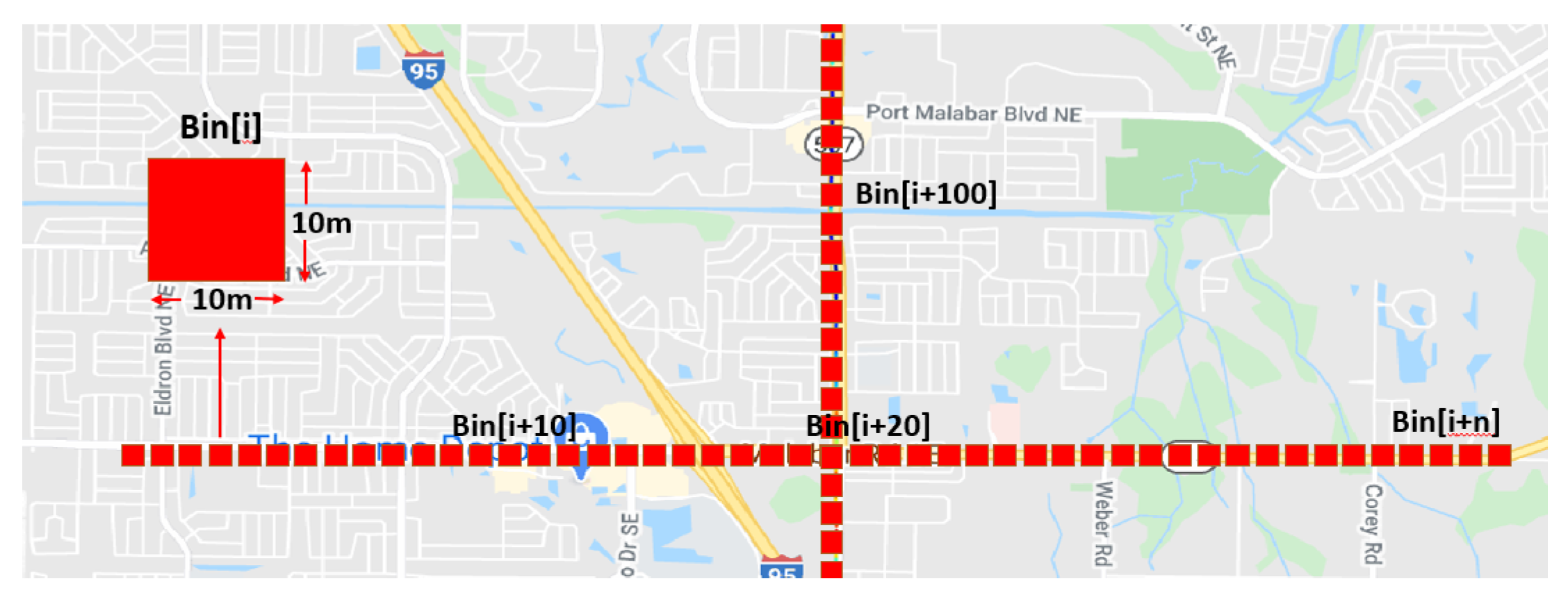
4.2. Data Binning

Data binning is a frequently used technique for minimizing minor measurement errors. This preprocessing procedure places data sequences into small clusters called bins, therefore, measurement fluctuations are decreased with the cost of resolution reduction. Data binning provides extra advantages by reducing the effect of car velocity in traffic. Since RF scanners gather a fixed amount of measurements in a period and predefined route, the number of the measurements decreases as the test car speeds up and proportionally increases as the car slows down or stops. Capturing more data points in some geographical areas, especially near traffic signs, affects ML algorithms and causes higher prediction errors. In this study, the geographical areas where the measured data set is divided into 10 m × 10 m bins after the feature extraction, and each bin exhibits the average values of the data features and parameters. Figure 6 shows how the data binning technique was applied for the drive testing scenario. The average RSRP and UL throughput values are assigned to $Bi{n}_{i+1}$, which indicates the bin value. Equation 10 shows the computation of $Bi{n}_{i+1}$ [36].

$${\overline{RSRP}}_{bi{n}_{i+1}}=\frac{1}{N_i}\sum _{i=1}^{N_i}RSR{P}_i$$

(10)

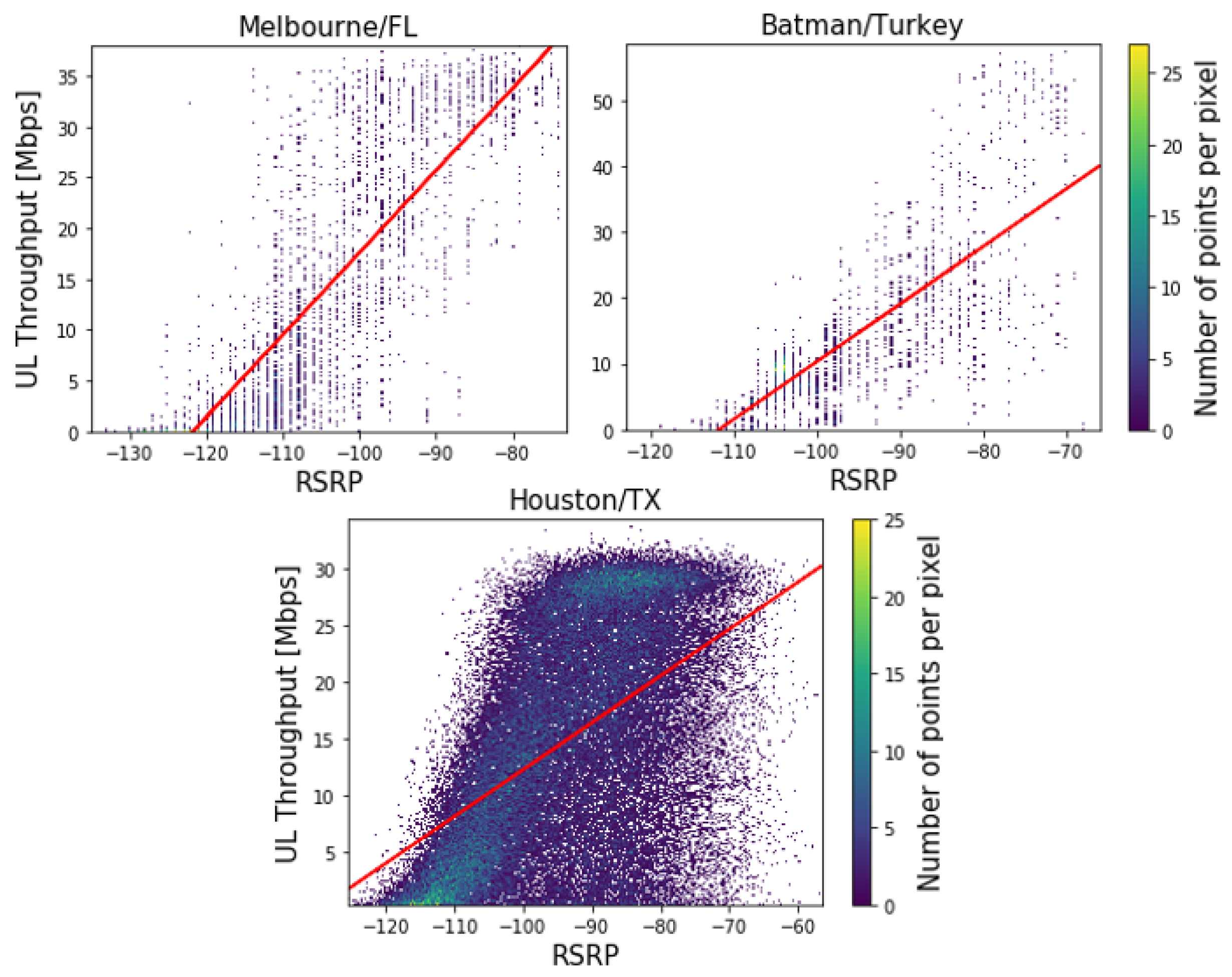
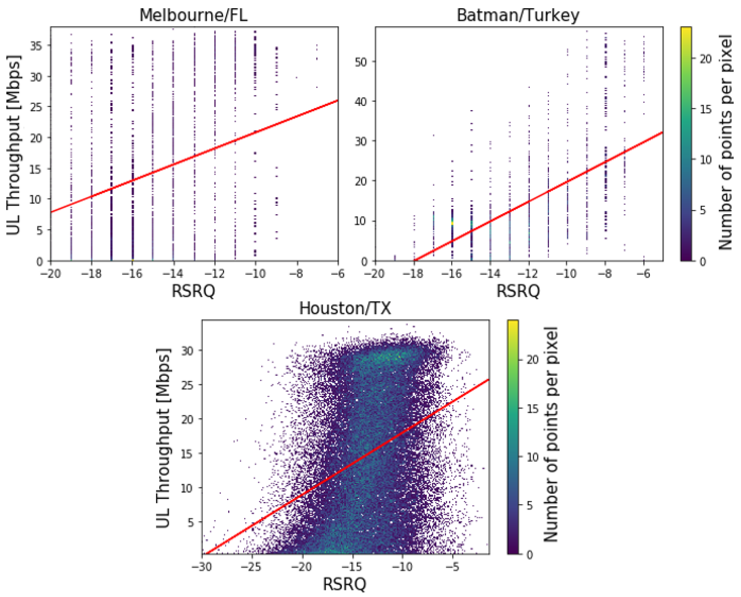
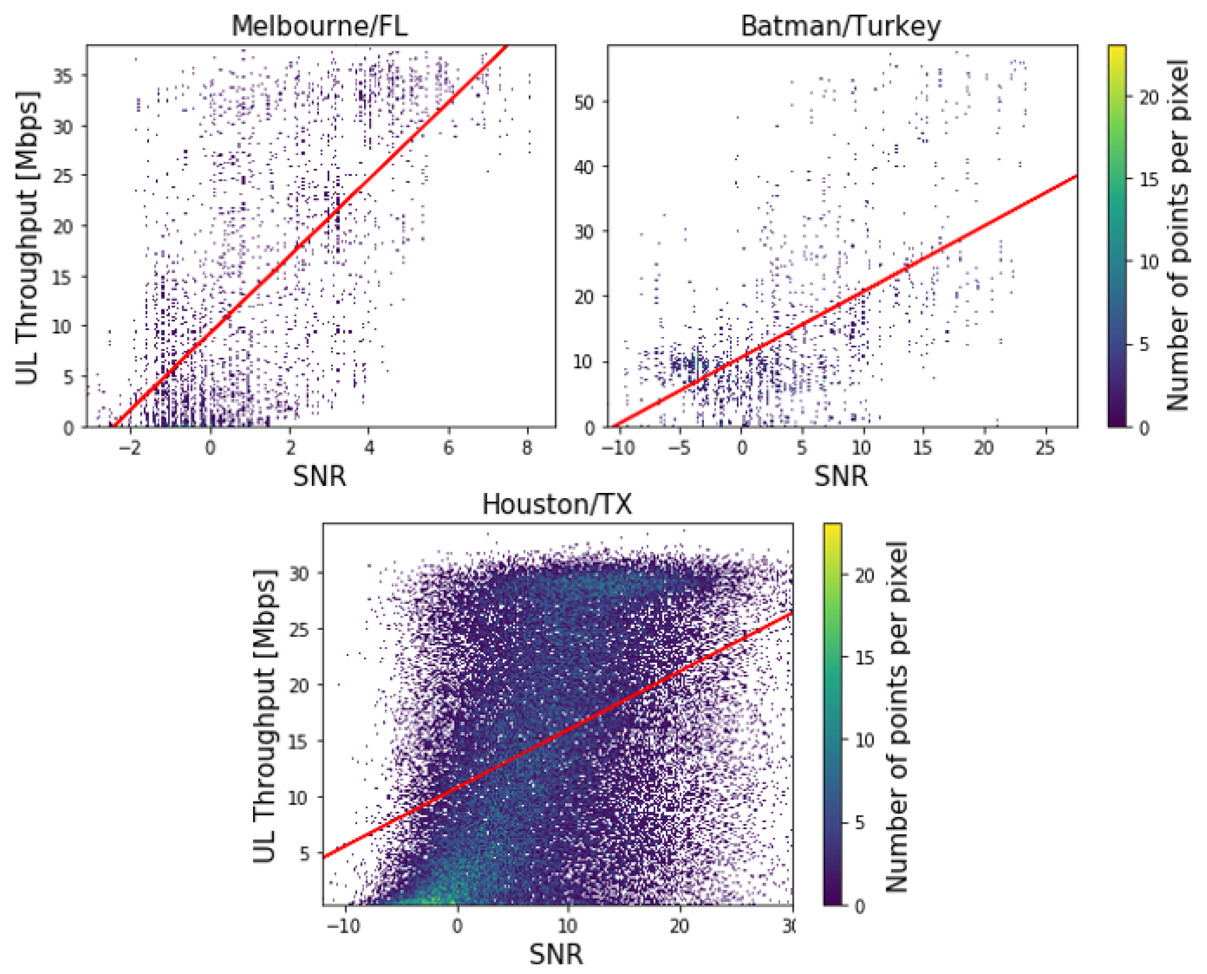
4.3. Correlation Analysis

Before the training/prediction stages, we implemented a correlation analysis to estimate each parameter’s importance on UL throughput. The first correlated feature, reference signal received power (RSRP), is the fundamental measurement for LTE coverage because it captures the received signal (in dBm) from a constant-power reference signal. This measurement is not affected by loading or interference. Thus, RSRP serves to estimate each radio cell tower’s coverage and is used for cell reselection and handover decisions. Since UL and DL are transmitted at different frequencies, signal levels fade independently, and high instantaneous RSRP levels do not necessarily indicate a strong UL signal. However, on average, RSRP readings capture coverage conditions that are partially reciprocal between UL and DL channels. For example, high RSRP readings show that UE is close to the cell tower, which is favorable for both UL and DL. Thus, in the absence of equivalent UL metrics, RSRP is correlated with UL throughput and a scatter plot of UL throughput as a function of RSRP. The RSRP relationship for each data set is presented in Figure 7.

The linear trend line is also included in the scatter plot graph showing the expected increase of UL throughput with growing RSRP levels. The RSRP measurements below −100 dBm are associated with lower UL throughputs, and the higher throughputs are concentrated in the uppermost RSRP regions. These apparent trends confirm that the RSRP analysis is useful in predicting the UL throughput. Reference signal received quality (RSRQ) is another fundamental LTE radio measurement. It captures the ratio between the received DL power from reference signal resource blocks of the serving cell and the total power in the DL direction, including all UEs in serving and adjacent cells. This ratio depends on the load in serving and adjacent cells and cannot be used to measure pure cell coverage directly. The RSRQ ranges are between −20 dB and −3 dB, where −20 dB indicates high interference and −3 dB indicates clear conditions with little interference. The scatter plot diagrams showing UL throughput as a function of the RSRQ are shown in Figure 8, together with the linear trend line.

While the trend line shows an expected increase with the RSRQ, the density of the points is not as clearly concentrated as in the RSRP comparison with the broader spreads at each RSRQ value. Therefore, the correlation between the UL throughput and RSRQ is expected to be lower than the correlation between the UL throughput and RSRP. The third LTE parameter with a high potential for accurate UL throughput prediction is signal-to-noise power (SNR). This metric applies to the baseband DL signal after down-conversion from the high-frequency wideband carrier. This measurement is expected to correlate closely with DL throughput and maintain a correlation with the UL throughput, although not directly, as in the DL direction. That is confirmed with measured data presented on the scatter plot in Figure 9 together with a linear regression line.

Measurements with low UL throughput are concentrated in the low SNR region, and the measurements with high UL throughput are grouped around higher SNR values. Therefore, SNR, similar to RSRP, is well correlated with UL throughput and will help predict the UL throughput. The correlations behind the scatter plots in Figure 7, Figure 8 and Figure 9 were calculated and are presented in

Table 1. Correlation Between UL Throughput and Received Signal Level (RSL).

Correlation with UL Throughput	LTE Parameters
	RSRP	RSRQ	SNR
Batman/Turkey	0.72	0.46	0.52
Melbourne/FL/USA	0.85	0.29	0.62
Houston/TX/USA	0.65	0.42	0.53

.

The coefficients were calculated using Spearman’s rank-order correlation since it is more robust to outliers than the common Pearson’s linear correlation and is preferred for describing dependency among parameters that are not normally distributed [37]. Spearman’s correlation factor ranges between −1 and +1. Values close to +1 indicate two parameters ranked closely together, near-zero values indicate weak correlation, and those near −1 indicate ranking in the opposite direction. where = Spearman’s rank-order correlation factor; n = number of data pairs.

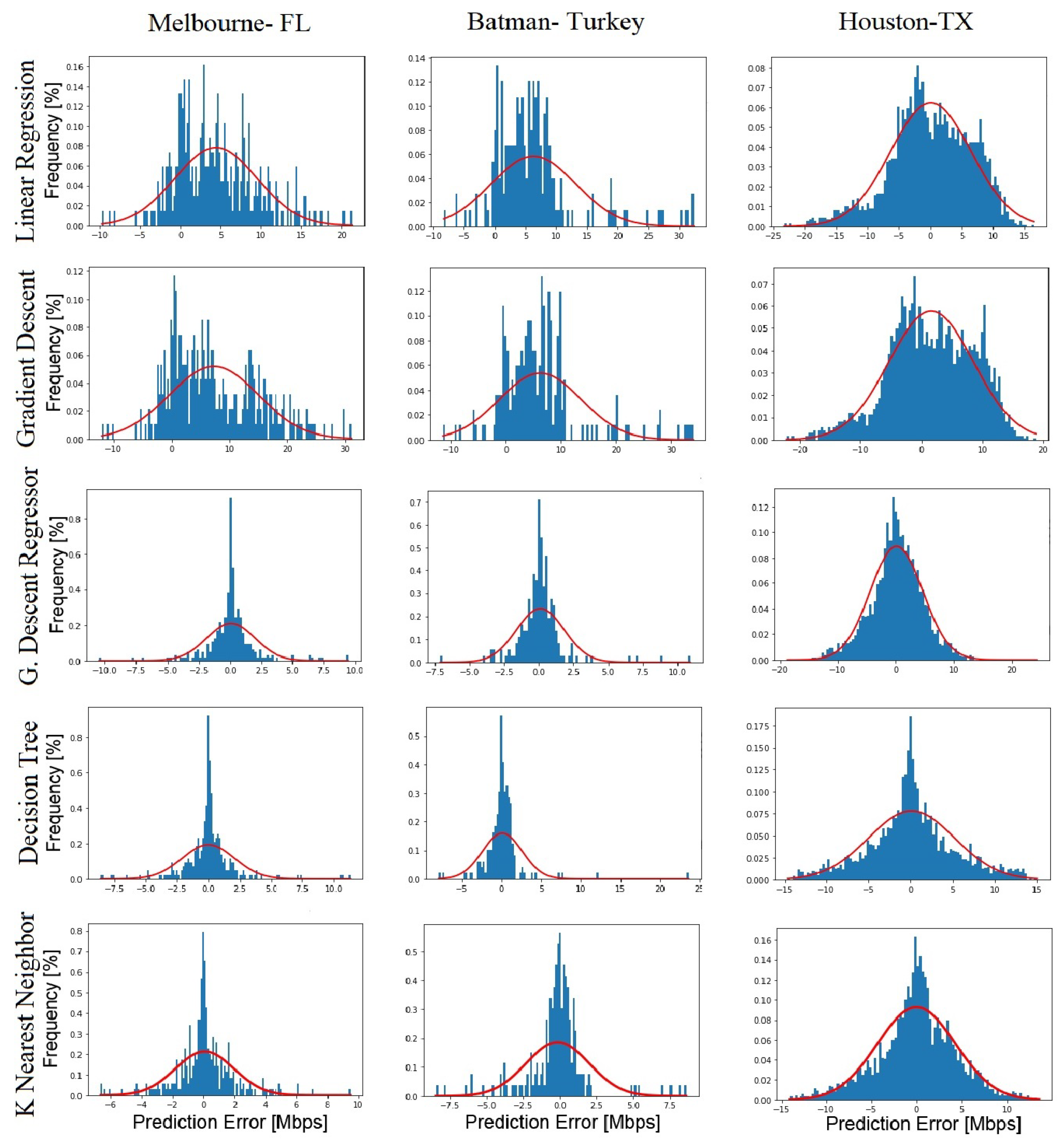
5. Prediction Results and Analysis

Three data sets collected over 10 days were divided into training and test sets where 90% of data were randomly assigned as a training set and fed into ML algorithms. The remaining data were used for the test set, which was used to assess the model prediction accuracy. The trained model was deployed on the test measurement subset to predict the UL throughput. Predicted UL throughputs were compared with test labels via the coefficient of determination $R^2$, as seen in Figure 10 and

Table 2. $R^2$ and MSE [Mbps] Analysis of ML Algorithms for Melbourne, FL, Batman, Turkey, and Houston, TX.

ML Algorithms	Melbourne		Batman		Houston
	${\mathit{R}}^2$	RMSE	${\mathit{R}}^2$	RMSE	${\mathit{R}}^2$	RMSE
LR	0.75	6.48	0.71	6.21	0.51	10.18
GD	0.75	6.44	0.71	6.16	0.51	10.03
GBR	0.91	3.81	0.86	4.12	0.66	8.08
DTR	0.92	3.74	0.86	4.13	0.67	8.19
KNN	0.92	3.76	0.85	4.24	0.69	6.60

.

According to Table 2 and Figure 10, DTR and KNN have the highest prediction accuracy among all ML algorithms. This highest prediction accuracy is likely because DTR and KNN both use classification while the others build mathematical models. Linear regression and gradient descent algorithms form a linear relationship between the LTE parameters and UL throughput. However, more intricate rules are needed to deduce this relationship instead of simple linearity and increase the prediction rate. GBR improves the prediction accuracy by implementing the residuals to the gradient descent method, and it provides almost as good RMSE as DTR and KNN algorithms. Moreover, we see a significant decrease in $R^2$ values from suburban to metropolitan areas. This decrease can be linked to scattering and fading effects in dense building areas. Additionally, Houston data might be affected by possible rain conditions, which might cause more estimation errors in this data set. Following the ML training and prediction, the variable’s importance of each parameter was investigated to rank features according to the impact on prediction accuracy. Calculated importance is illustrated in the bar chart in Figure 11.

It confirms that the RSRP metric is the main contributor (over 60%) to the prediction algorithm, while baseband SNR and RSRQ have almost equal importance (between 9 to 20%). According to DTR results, the prediction feature importance levels are drawn using Python sckit-learn library.

6. Limitation and Discussion

The gradual closure of the channel capacity asymmetry between the UL and the DL with developing and widespread technologies has shown that intensive research on the DL channel basis should also be performed in the UL direction. This article aimed to make channel estimation with a robust and high accuracy prediction rate using as few LTE parameters as possible. In the system, physical layer parameters must be obtained via receivers or scanners located in the experiment area to estimate the UL throughput of a specific location. However, receivers and scanners may not represent the exact measurements as phones because of the differences in antenna gain. Therefore, the proposed method should also be performed by mobile phones to see whether there is a significant change in measurements. Moreover, regarding sustainable and high-quality network services, the proposed method is essential in providing adequate bandwidth and higher UL throughput rates, which may be needed at shopping malls, concerts, fairs, and crowded areas. The proposed method will estimate the required UL throughput and may be used to adjust the DL-UL channel bandwidth allocation asymmetry in favor of UL. In other words, the allocated DL channel bandwidth can be shifted to the UL channel when needed. Finally, it should be emphasized that most of the studies focused on DL channel prediction, and a few of the studies have performed UL throughput prediction with low prediction accuracy (83–94%). The measurements of these studies are collected from the same environment, which may limit their general usage in different environments.

7. Conclusions

This research presented an ML-based UL throughput prediction model, which applies to 4G and possibly, 5G mobile networks. The data sets were collected through drive tests on currently deployed 4G LTE mobile networks in different locations (Melbourne, FL, Batman, Turkey, Houston, TX), and the performance of ML algorithms such as linear regression, gradient descent, gradient boosting regression, decision tree regression, and k-nearest neighbor models were tested on UL throughput prediction. An enhanced ML traffic management is modeled based on minimal feature sets such as RSRP, RSRQ, and SNR. The highest correlation is observed with RSRP 0.85 in Melbourne, FL, RSRQ 0.46 in Batman, Turkey, and SNR 0.53 in Melbourne, FL. The determination coefficient ($R^2$) values were calculated along with RMSE values. The observed coefficient of determination was 0.92 for both DTR and KNN algorithms. It is also seen that it is likely to observe a relationship between UL throughput prediction accuracy and the environment’s type since $R^2$ values decrease from 0.92 to 0.69 from suburban areas to metropolitan areas. However, more research needs to be conducted with additional data to support this result.

References

1. Kim, Y.; Kim, Y.; Oh, J.; Ji, H.; Yeo, J.; Choi, S.; Ryu, H.; Noh, H.; Kim, T.; Lee, J.; et al. New Radio (NR) and its Evolution toward 5G-Advanced. IEEE Wirel. Commun. 2019, 26, 2–7. [Google Scholar] [CrossRef]
2. Hajlaoui, E.; Khlifi, A.; Zaier, A.; Ghodhbane, J.; Hamed, M.B.; Sbita, L. Performance Evaluation of LTE Physical Layer. In Proceedings of the 2019 International Conference on Internet of Things, Embedded Systems and Communications (IINTEC), Tunis, Tunisia, 20–22 December 2019; pp. 106–111. [Google Scholar] [CrossRef]
3. Singh, H.; Prasad, R.; Bonev, B. The Studies of Millimeter Waves at 60 GHz in Outdoor Environments for IMT Applications: A State of Art. Wireless Pers. Commun. 2018, 100, 463–474. [Google Scholar] [CrossRef] [Green Version]
4. Isyaku, B.; Mohd Zahid, M.S.; Bte Kamat, M.; Abu Bakar, K.; Ghaleb, F.A. Software Defined Networking Flow Table Management of OpenFlow Switches Performance and Security Challenges: A Survey. Future Internet 2020, 12, 147. [Google Scholar] [CrossRef]
5. Lutu, A.; Perino, D.; Bagnulo, M.; Frias-Martinez, E.; Khangosstar, J. A Characterization of the COVID-19 Pandemic Impact on a Mobile Network Operator Traffic. In Proceedings of the IMC ’20: ACM Internet Measurement Conference, Virtual Event, USA, 27–29 October 2020. [Google Scholar]
6. Edler, G.; Wang, L.; Horiuchi, A. Special Subframe Configuration for Latency Reduction. U.S. Patent Application No. 16/089,279, 26 October 2021. [Google Scholar]
7. Rayal, F. LTE in a Nutshell. 2020. Available online: https://home.zhaw.ch/kunr/NTM1/literatur/LTE%20in%20a%20Nutshell%20-%20Physical%20Layer.pdf (accessed on 24 October 2020).
8. Teng, Y.; Yan, M.; Liu, D.; Han, Z.; Song, M. Distributed Learning Solution for Uplink Traffic Control in Energy Harvesting Massive Machine-Type Communications. IEEE Wirel. Commun. Lett. 2020, 9, 485–489. [Google Scholar] [CrossRef]
9. Kim, T.; Jung, B.C. Performance Analysis of Grant-Free Multiple Access for Supporting Sporadic Traffic in Massive IoT Networks. IEEE Access 2019, 7, 166648–166656. [Google Scholar] [CrossRef]
10. Kim, T.; Song, T.; Kim, W.; Pack, S. Phase-Divided MAC Protocol for Integrated Uplink and Downlink Multiuser MIMO WLANs. IEEE Trans. Veh. Technol. 2018, 67, 3172–3185. [Google Scholar] [CrossRef]
11. Xu, C.; Wu, M.; Xu, Y.; Xu, Y. Shortest Uplink Scheduling for NOMA-Based Industrial Wireless Networks. IEEE Syst. J. 2020, 14, 5384–5395. [Google Scholar] [CrossRef]
12. Ma, Z.; Feng, L.; Wang, Z. Supporting Asymmetric Transmission for Full-Duplex Smart-Home Networks. IEEE Access 2019, 7, 34807–34822. [Google Scholar] [CrossRef]
13. Sun, K.; Wu, J.; Huang, W.; Zhang, H.; Hsieh, H.-Y.; Leung, V.C.M. Uplink Performance Improvement for Downlink-Uplink Decoupled HetNets with Non-Uniform User Distribution. IEEE Trans. Veh. Technol. 2020, 69, 7518–7530. [Google Scholar] [CrossRef]
14. Jiménez, L.R.; Solera, M.; Toril, M.; Luna-Ramírez, S.; Bejarano-Luque, J.L. The Upstream Matters: Impact of Uplink Performance on YouTube 360° Live Video Streaming in LTE. IEEE Access 2021, 9, 123245–123259. [Google Scholar] [CrossRef]
15. Homssi, B.A.; Al-Hourani, A. Modeling Uplink Coverage Performance in Hybrid Satellite-Terrestrial Networks. IEEE Commun. Lett. 2021, 25, 3239–32431. [Google Scholar] [CrossRef]
16. Ali, S.; Rajatheva, N.; Saad, W. Fast Uplink Grant for Machine Type Communications: Challenges and Opportunities. IEEE Commun. Mag. 2019, 57, 97–103. [Google Scholar] [CrossRef] [Green Version]
17. Shen, H.; Ye, Q.; Zhuang, W.; Shi, W.; Bai, G.; Yang, G. Drone-Small-Cell-Assisted Resource Slicing for 5G Uplink Radio Access Networks. IEEE Trans. Veh. Technol. 2021, 70, 7071–7086. [Google Scholar] [CrossRef]
18. Ruan, L.; Dias, M.P.I.; Wong, E. SmartBAN With Periodic Monitoring Traffic: A Performance Study on Low Delay and High Energy Efficiency. IEEE J. Biomed. Health Inform. 2018, 22, 471–482. [Google Scholar] [CrossRef]
19. Carson, S.; Lundvall, A. Mobility on The Pulse of The Networked Society; Ericsson: Stockholm, Sweden, 2016; pp. 1–36. [Google Scholar]
20. Kato, N.; Mao, B.; Tang, F.; Kawamoto, Y.; Liu, J. Ten Challenges in Advancing Machine Learning Technologies toward 6G. IEEE Wirel. Commun. 2020, 27, 96–103. [Google Scholar] [CrossRef]
21. Egi, Y.; Otero, C.E. Machine-Learning and 3D Point-Cloud Based Signal Power Path Loss Model for the Deployment of Wireless Communication Systems. IEEE Access 2019, 7, 42507–42517. [Google Scholar] [CrossRef]
22. Ray, P.P.; Nguyen, K. A Review on Blockchain for Medical Delivery Drones in 5G-IoT Era: Progress and Challenges. In Proceedings of the 2020 IEEE/CIC International Conference on Communications in China (ICCC Workshops), Chongqing, China, 9–11 August 2020; pp. 29–34. [Google Scholar] [CrossRef]
23. Yue, C.; Jin, R.; Suh, K.; Qin, Y.; Wang, B.; Wei, W. LinkForecast: Cellular Link Bandwidth Prediction in LTE Networks. IEEE Trans. Mob. Comput. 2018, 17, 1582–1594. [Google Scholar] [CrossRef]
24. Jomrich, F.; Herzberger, A.; Meuser, T.; Richerzhagen, B.; Steinmetz, R.; Wille, C. Cellular bandwidth prediction for highly automated driving evaluation of machine learning approaches based on real-world data. In Proceedings of the VEHITS 2018—International Conference on Vehicle Technology and Intelligent Transport Systems, Funchal-Madeira, Portugal, 16–18 March 2018; pp. 121–132. [Google Scholar]
25. Bojovic, B.; Meshkova, E.; Baldo, N.; Riihijarvi, J.; Petrova, M. Machine learning-based dynamic frequency and bandwidth allocation in self-organized LTE dense small cell deployments. Eurasip J. Wirel. Commun. Netw. 2016, 2016, 1–16. [Google Scholar] [CrossRef] [Green Version]
26. Oussakel, I.; Owezarski, P.; Berthou, P. Experimental Estimation of LTE-A Performance. In Proceedings of the 2019 15th International Conference on Network and Service Management (CNSM), Halifax, NS, Canada, 21–25 October 2019. [Google Scholar]
27. Awad, W.A.; ELseuofi, S.M. Machine Learning methods for E-mail Classification. Int. J. Comput. Appl. 2011, 16, 39–45. [Google Scholar] [CrossRef] [Green Version]
28. Hasan, M.; Islam, M.M.; Zarif, M.I.I.; Hashem, M.M.A. Attack and anomaly detection in IoT sensors in IoT sites using machine learning approaches. Internet Things 2019, 7, 100059. [Google Scholar] [CrossRef]
29. Olukan, T.A.; Chiou, Y.C.; Chiu, C.H.; Lai, C.Y.; Santos, S.; Chiesa, M. Predicting the suitability of lateritic soil type for low cost sustainable housing with image recognition and machine learning techniques. J. Build. Eng. 2000, 29, 101175. [Google Scholar] [CrossRef]
30. Ketkar, N. Stochastic Gradient Descent. In Deep Learning with Python; Apress: Berkeley, CA, USA, 2017; pp. 113–132. [Google Scholar]
31. Li, C. A Gentle Introduction to Gradient Boosting. 2016. Available online: http://www.ccs.neu.edu/home/vip/teach/MLcourse/4boosting/slides/gradient-boosting.pdf (accessed on 5 November 2021).
32. Wang, F.; Wang, Q.; Nie, F.; Li, Z.; Yu, W.; Ren, F. A linear multivariate binary decision tree classifier based on K-means splitting. Pattern Recognit. 2020, 107, 107521. [Google Scholar] [CrossRef]
33. Kramer, O. K-Nearest Neighbors. In Dimensionality Reduction with Unsupervised Nearest Neighbors. In Intelligent Systems Reference Library; Springer: Berlin/Heidelberg, 2013; Volume 51. [Google Scholar] [CrossRef]
34. SinghAn, A. K-Nearest Neighbors Algorithm: KNN Regression Python. 2020. Available online: https://www.analyticsvidhya.com/blog/2018/08/k-nearest-neighbor-introduction-regression-python/ (accessed on 4 November 2020).
35. Christodoulou, C.; Moorby, J.M.; Tsiplakou, E.; Kantas, D.; Foskolos, A. Evaluation of nitrogen excretion equations for ryegrass pasture-fed dairy cows. Animal 2021, 15, 100311. [Google Scholar] [CrossRef] [PubMed]
36. Egi, Y.; Eyceyurt, E.; Kostanic, I.; Otero, C.E. An Efficient Approach for Evaluating Performance in LTE Wireless Networks. In Proceedings of the International Conference on Wireless Networks (ICWN); The Steering Committee of the World Congress in Computer Science, Computer Engineering and Applied Computing (WorldComp): Las Vegas, NV, USA, 2017; pp. 48–54. [Google Scholar]
37. Mehta, D.S.; Chen, S. A spearman correlation based star pattern recognition. In Proceedings of the IEEE International Conference on Image Processing (ICIP), Beijing, China, 17–20 September 2017. [Google Scholar]
Figure 1. Illustration of the learning process.
Electronics 11 01227 g001
Figure 2. Demonstration of gradient descent.
Electronics 11 01227 g002
Figure 3. Representation of a DT.
Electronics 11 01227 g003
Figure 4. Training and feedback mechanism of the prediction models.
Electronics 11 01227 g004
Figure 5. Geomap visualization of UL throughput.
Electronics 11 01227 g005
Figure 6. Representation of data binning.
Electronics 11 01227 g006
Figure 7. Scatter plot of RSRP and UL throughput.
Electronics 11 01227 g007
Figure 8. Scatter plot of RSRQ and UL throughput.
Electronics 11 01227 g008
Figure 9. Scatter plot of SNR and UL throughput.
Electronics 11 01227 g009
Figure 10. Prediction Algorithm Comparison.
Electronics 11 01227 g010
Figure 11. Variable Importance.
Electronics 11 01227 g011