
Multi-Task Learning Using Gradient Balance and Clipping with an Application in Joint Disparity Estimation and Semantic Segmentation


Abstract
:1. Introduction
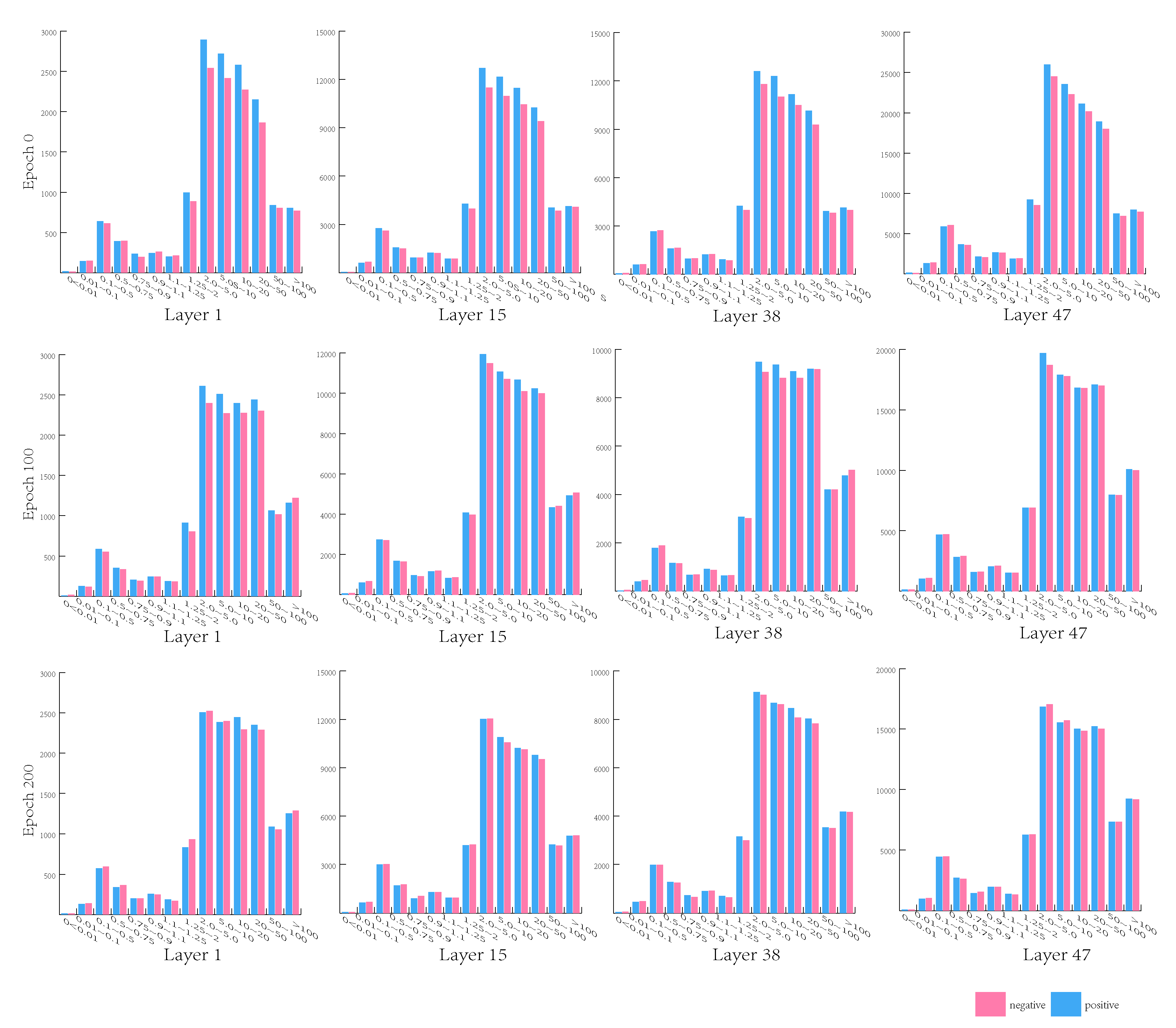
- We have a deep analysis of the feature learning in MTL and find that mutual feature learning among the backbone network is important for the final performance. Furthermore, we introduce a novel learning method from the angle of gradient descent to avoid complex network design and elaborate loss weights adjustment.
- We propose an MTSGD method to optimize multi-task learning from the perspective of considering multi-task learning as an optimization problem. We decompose the multiple task gradient into task-specific sub-gradient and leverage the proposed gradient clipping operation to balance the contribution of each sub-gradient.
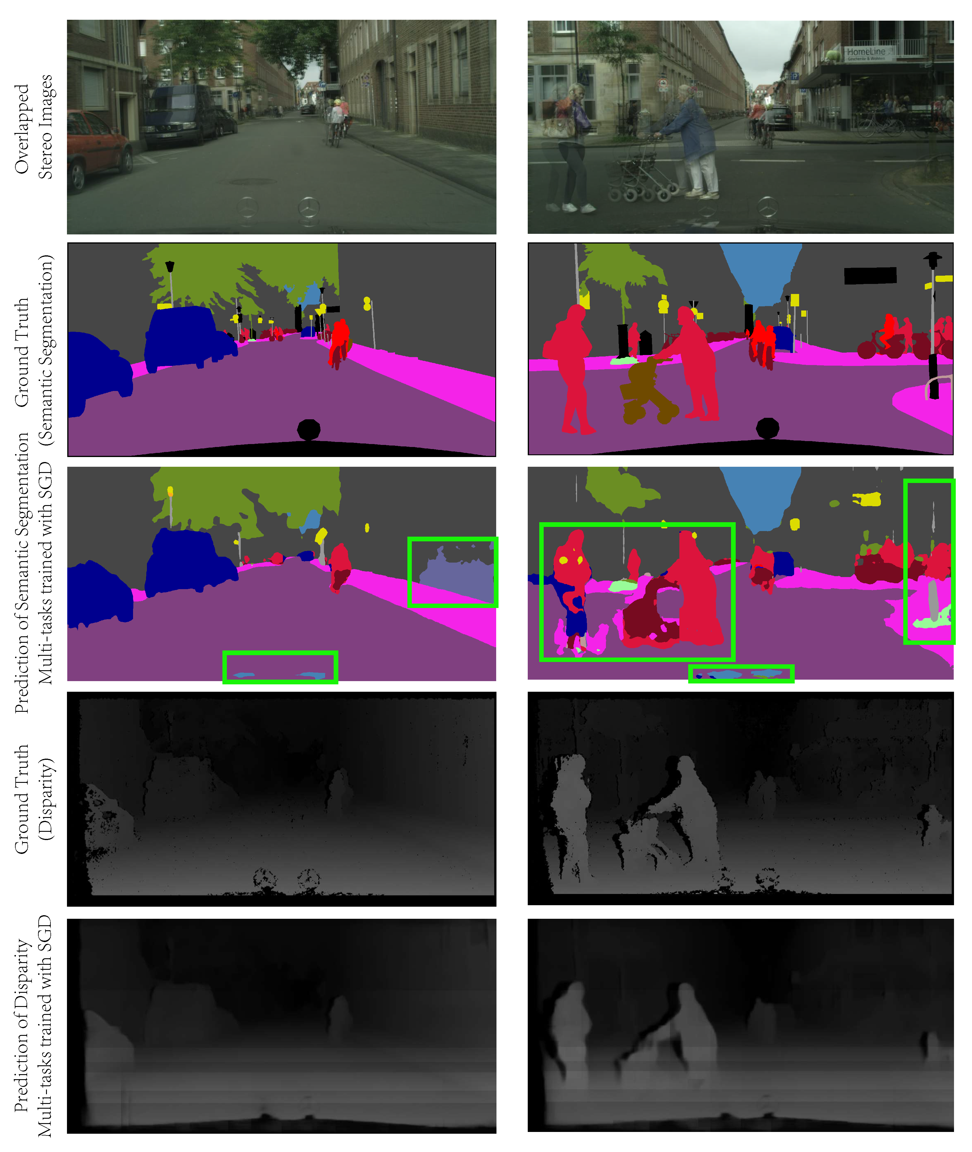
- We evaluate the proposed method on the challenging MTL case: joint learning of disparity estimation and semantic segmentation. Experiment results on the benchmark dataset validate the effectiveness of the proposed MTSGD.
2. Related Work
3. Optimizer for Multi-Task Learning
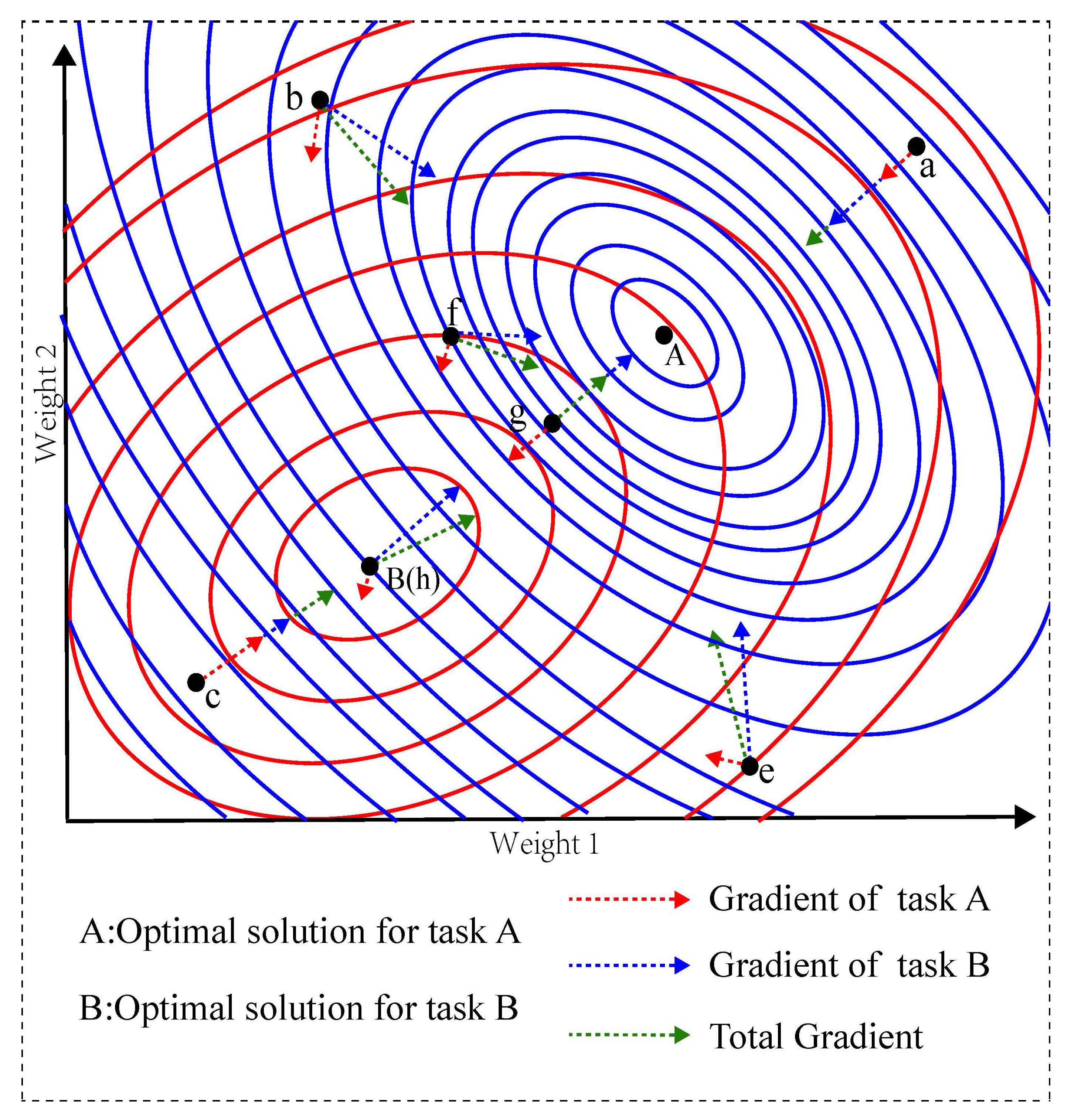
3.1. Important Observation
3.2. Multi-Task Stochastic Gradient Descent
4. Experiment
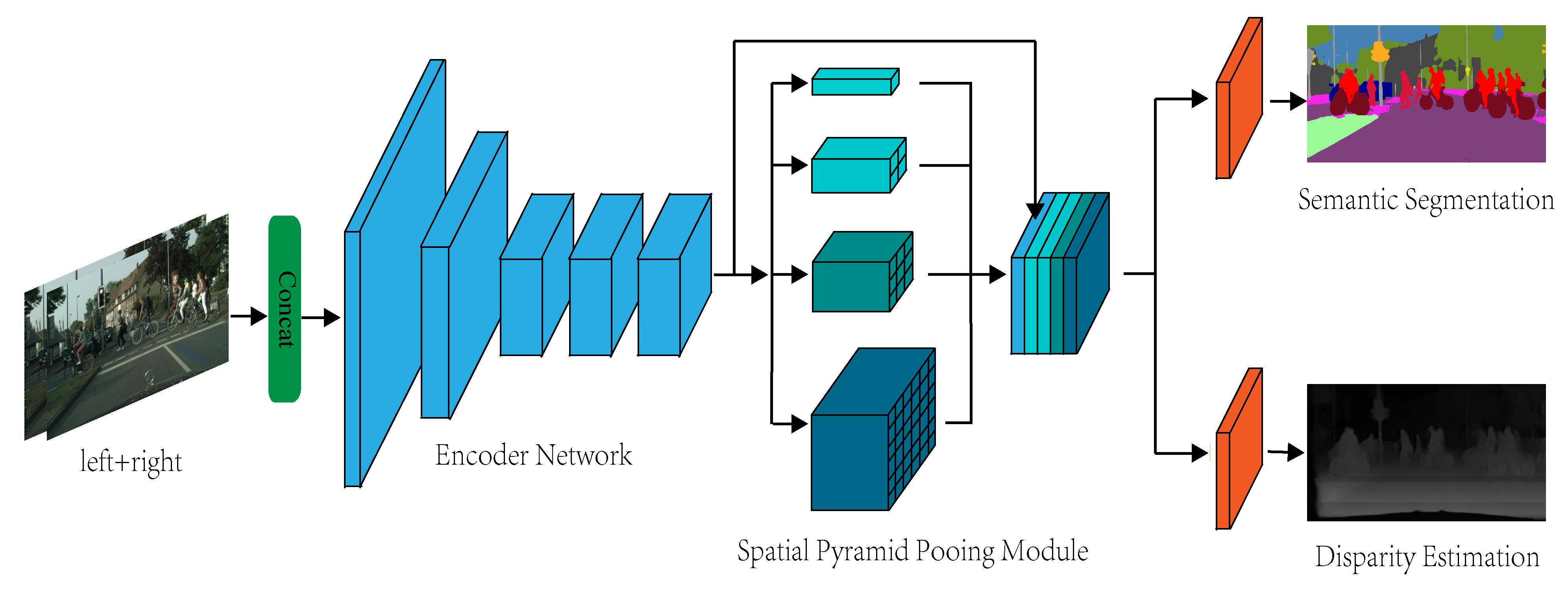
4.1. Overall Network Architecture
4.2. Experimental Settings
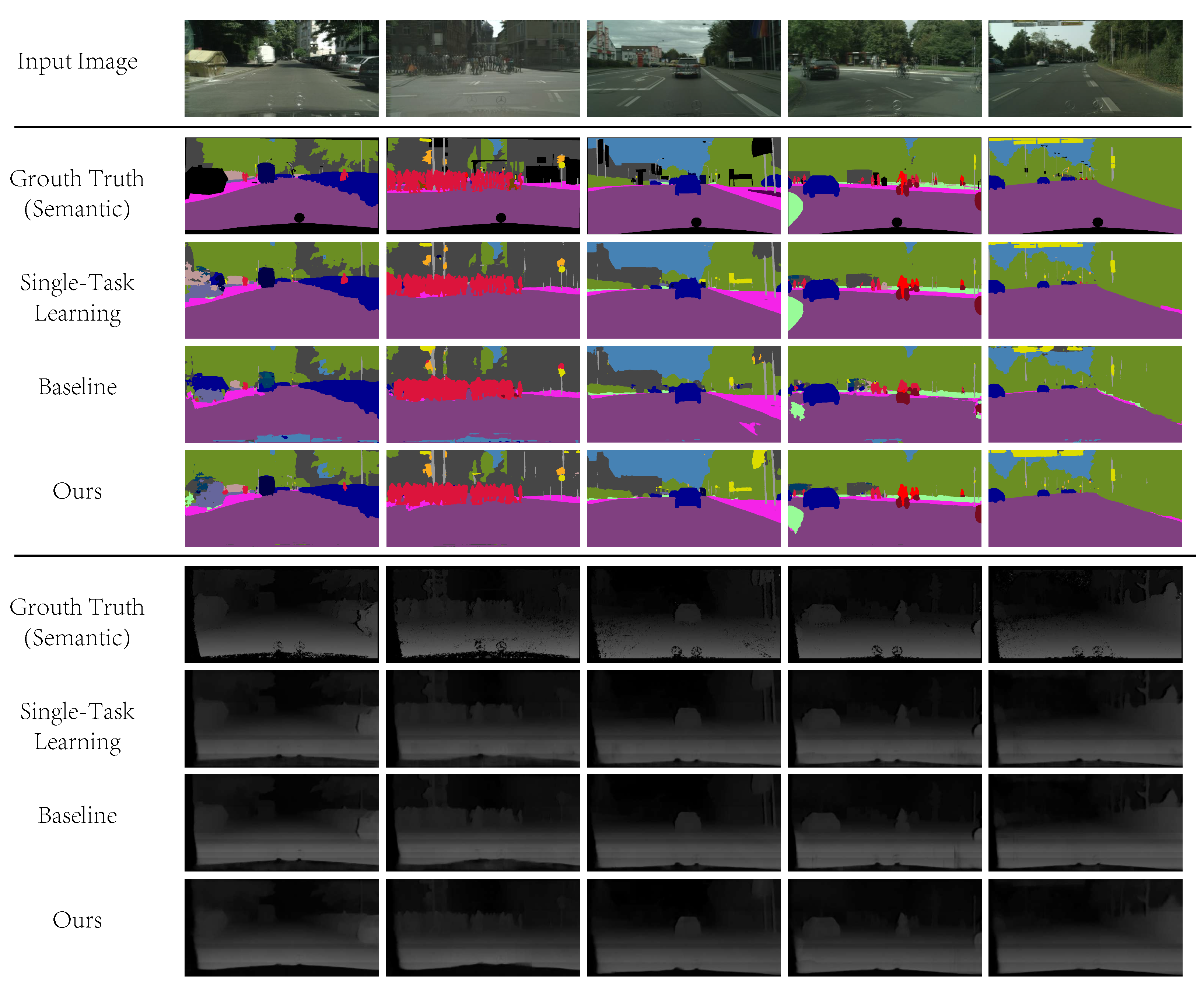
4.3. Experimental Results
4.4. Ablation Studies
4.5. Discussion
5. Conclusions
Author Contributions
Funding
Acknowledgments
Conflicts of Interest
References
- Russakovsky, O.; Deng, J.; Su, H.; Krause, J.; Satheesh, S.; Ma, S.; Huang, Z.; Karpathy, A.; Khosla, A.; Bernstein, M.; et al. ImageNet Large Scale Visual Recognition Challenge. Int. J. Comput. Vis. 2015, 115, 211–252. [Google Scholar] [CrossRef] [Green Version]
- He, K.; Zhang, X.; Ren, S.; Sun, J. Deep residual learning for image recognition. In Proceedings of the IEEE Conference on Computer Vision and pattern Recognition, Las Vegas, NV, USA, 27–30 June 2016; pp. 770–778. [Google Scholar]
- Hu, J.; Shen, L.; Sun, G. Squeeze-and-Excitation Networks. In Proceedings of the IEEE Conference on Computer Vision and Pattern Recognition, 18–23 June 2018; pp. 7132–7141. [Google Scholar]
- Ren, S.; He, K.; Girshick, R.; Sun, J. Faster r-cnn: Towards real-time object detection with region proposal networks. Adv. Neural Inf. Process. Syst. 2015, 1, 91–99. [Google Scholar] [CrossRef] [PubMed] [Green Version]
- He, K.; Gkioxari, G.; Dollár, P.; Girshick, R. Mask r-cnn. In Proceedings of the IEEE International Conference on Computer Vision, Venice, Italy, 22–29 October 2017; pp. 2961–2969. [Google Scholar]
- Lin, T.; Dollar, P.; Girshick, R.B.; He, K.; Hariharan, B.; Belongie, S.J. Feature Pyramid Networks for Object Detection. In Proceedings of the 30th IEEE Conference on Computer Vision and Pattern Recognition, CVPR 2017, Honolulu, HI, USA, 21–26 July 2017; pp. 936–944. [Google Scholar]
- Long, J.; Shelhamer, E.; Darrell, T. Fully convolutional networks for semantic segmentation. In Proceedings of the IEEE Conference on Computer Vision and Pattern Recognition, Boston, MA, USA, 7–12 June 2015; pp. 3431–3440. [Google Scholar]
- Zhao, H.; Shi, J.; Qi, X.; Wang, X.; Jia, J. Pyramid scene parsing network. In Proceedings of the 2017 IEEE Conference on Computer Vision and Pattern Recognition, Honolulu, HI, USA, 21–26 July 2017; pp. 2881–2890. [Google Scholar]
- Chen, L.C.; Papandreou, G.; Schroff, F.; Adam, H. Rethinking atrous convolution for semantic image segmentation. arXiv 2017, arXiv:1706.05587. [Google Scholar]
- Zhang, Z.; Cui, Z.; Xu, C.; Yan, Y.; Sebe, N.; Yang, J. Pattern-Affinitive Propagation across Depth, Surface Normal and Semantic Segmentation. In Proceedings of the IEEE Conference on Computer Vision and Pattern Recognition, Long Beach, CA, USA, 16–17 June 2019; pp. 4106–4115. [Google Scholar]
- Xu, D.; Ouyang, W.; Wang, X.; Sebe, N. Pad-net: Multi-tasks guided prediction-and-distillation network for simultaneous depth estimation and scene parsing. In Proceedings of the IEEE Conference on Computer Vision and Pattern Recognition, Salt Lake City, UT, USA, 28–23 June 2018; pp. 675–684. [Google Scholar]
- Yin, Z.; Shi, J. Geonet: Unsupervised learning of dense depth, optical flow and camera pose. In Proceedings of the IEEE Conference on Computer Vision and Pattern Recognition, Salt Lake City, UT, USA, 28–23 June 2018; pp. 1983–1992. [Google Scholar]
- Liu, S.; Johns, E.; Davison, A.J. End-to-end multi-task learning with attention. In Proceedings of the IEEE Conference on Computer Vision and Pattern Recognition, Long Beach, CA, USA, 15–20 June 2019; pp. 1871–1880. [Google Scholar]
- Bragman, F.J.; Tanno, R.; Ourselin, S.; Alexander, D.C.; Cardoso, J. Stochastic Filter Groups for Multi-Task CNNs: Learning Specialist and Generalist Convolution Kernels. In Proceedings of the IEEE International Conference on Computer Vision (ICCV), Seoul, Korea, 27 October–2 November 2019. [Google Scholar]
- Guo, M.; Haque, A.; Huang, D.A.; Yeung, S.; Fei-Fei, L. Dynamic task prioritization for multitask learning. In Proceedings of the European Conference on Computer Vision (ECCV), Munich, Germany, 8–14 September 2018; pp. 270–287. [Google Scholar]
- Chen, Z.; Badrinarayanan, V.; Lee, C.Y.; Rabinovich, A. Gradnorm: Gradient normalization for adaptive loss balancing in deep multitask networks. arXiv 2017, arXiv:1711.02257. [Google Scholar]
- Pang, J.; Sun, W.; Ren, J.S.; Yang, C.; Yan, Q. Cascade residual learning: A two-stage convolutional neural network for stereo matching. In Proceedings of the IEEE International Conference on Computer Vision, Venice, Italy, 22–29 October 2017; pp. 887–895. [Google Scholar]
- Chang, J.R.; Chen, Y.S. Pyramid stereo matching network. In Proceedings of the IEEE Conference on Computer Vision and Pattern Recognition, Salt Lake City, UT, USA, 28–23 June 2018; pp. 5410–5418. [Google Scholar]
- Cheng, X.; Wang, P.; Yang, R. Depth estimation via affinity learned with convolutional spatial propagation network. In Proceedings of the European Conference on Computer Vision (ECCV), Munich, Germany, 8–14 September 2018; pp. 103–119. [Google Scholar]
- Ronneberger, O.; Fischer, P.; Brox, T. U-Net: Convolutional Networks for Biomedical Image Segmentation. In Medical Image Computing and Computer Assisted Intervention; Navab, N., Hornegger, J., Wells, W.M., Frangi, A.F., Eds.; Springer: Cham, Switzerland, 2015; pp. 234–241. [Google Scholar]
- Peng, C.; Zhang, X.; Yu, G.; Luo, G.; Sun, J. Large Kernel Matters–Improve Semantic Segmentation by Global Convolutional Network. In Proceedings of the IEEE Conference on Computer Vision and Pattern Recognition, Honolulu, HI, USA, 21–26 July 2017; pp. 4353–4361. [Google Scholar]
- Chen, L.C.; Papandreou, G.; Kokkinos, I.; Murphy, K.; Yuille, A.L. Semantic image segmentation with deep convolutional nets and fully connected crfs. arXiv 2014, arXiv:1412.7062. [Google Scholar]
- Chen, L.C.; Papandreou, G.; Kokkinos, I.; Murphy, K.; Yuille, A.L. Deeplab: Semantic image segmentation with deep convolutional nets, atrous convolution, and fully connected crfs. IEEE Trans. Pattern Anal. Mach. Intell. 2017, 40, 834–848. [Google Scholar] [CrossRef] [PubMed] [Green Version]
- Chen, L.C.; Zhu, Y.; Papandreou, G.; Schroff, F.; Adam, H. Encoder-decoder with atrous separable convolution for semantic image segmentation. In Proceedings of the European Conference on Computer Vision (ECCV), Munich, Germany, 8–14 September 2018; pp. 801–818. [Google Scholar]
- Tian, Z.; He, T.; Shen, C.; Yan, Y. Decoders Matter for Semantic Segmentation: Data-Dependent Decoding Enables Flexible Feature Aggregation. In Proceedings of the IEEE Conference on Computer Vision and Pattern Recognition, Long Beach, CA, USA, 15–20 June 2019; pp. 3126–3135. [Google Scholar]
- Mayer, N.; Ilg, E.; Hausser, P.; Fischer, P.; Cremers, D.; Dosovitskiy, A.; Brox, T. A large dataset to train convolutional networks for disparity, optical flow, and scene flow estimation. In Proceedings of the IEEE Conference on Computer Vision and Pattern Recognition, Las Vegas, NV, USA, 27–30 June 2016; pp. 4040–4048. [Google Scholar]
- Kendall, A.; Martirosyan, H.; Dasgupta, S.; Henry, P.; Kennedy, R.; Bachrach, A.; Bry, A. End-to-end learning of geometry and context for deep stereo regression. In Proceedings of the IEEE International Conference on Computer Vision, Venice, Italy, 22–29 October 2017; pp. 66–75. [Google Scholar]
- Eigen, D.; Puhrsch, C.; Fergus, R. Depth map prediction from a single image using a multi-scale deep network. Adv. Neural Inf. Process. Syst. 2014, 2366–2374. [Google Scholar]
- Liu, F.; Shen, C.; Lin, G.; Reid, I. Learning depth from single monocular images using deep convolutional neural fields. IEEE Trans. Pattern Anal. Mach. Intell. 2015, 38, 2024–2039. [Google Scholar] [CrossRef] [PubMed] [Green Version]
- Kocabas, M.; Karagoz, S.; Akbas, E. Multiposenet: Fast multi-person pose estimation using pose residual network. In Proceedings of the European Conference on Computer Vision (ECCV), Munich, Germany, 8–14 September 2018; pp. 417–433. [Google Scholar]
- Strezoski, G.; Noord, N.v.; Worring, M. Many Task Learning With Task Routing. In Proceedings of the IEEE International Conference on Computer Vision (ICCV), Seoul, Korea, 27–28 October 2019. [Google Scholar]
- Kundu, J.N.; Lakkakula, N.; Babu, R.V. UM-Adapt: Unsupervised Multi-Task Adaptation Using Adversarial Cross-Task Distillation. In Proceedings of the IEEE International Conference on Computer Vision (ICCV), Long Beach, CA, USA, 15–20 June 2019. [Google Scholar]
- Jha, A.; Kumar, A.; Banerjee, B.; Chaudhuri, S. Adamt-net: An adaptive weight learning based multi-task learning model for scene understanding. In Proceedings of the IEEE Conference on Computer Vision and Pattern Recognition (CVPR), Long Beach, CA, USA, 15–20 June 2019; pp. 3027–3035. [Google Scholar]
- Cordts, M.; Omran, M.; Ramos, S.; Rehfeld, T.; Enzweiler, M.; Benenson, R.; Franke, U.; Roth, S.; Schiele, B. The Cityscapes Dataset for Semantic Urban Scene Understanding. In Proceedings of the IEEE Conference on Computer Vision and Pattern Recognition (CVPR), Las Vegas, NV, USA, 27–30 June 2016. [Google Scholar]
- Liu, W.; Rabinovich, A.; Berg, A.C. Parsenet: Looking wider to see better. arXiv 2015, arXiv:1506.04579. [Google Scholar]
- Yu, F.; Koltun, V. Multi-scale context aggregation by dilated convolutions. arXiv 2015, arXiv:1511.07122. [Google Scholar]
- Zbontar, J.; LeCun, Y. MStereo matching by training a convolutional neural network to compare image patches. J. Mach. Learn. Res. 2016, 17, 2287–2318. [Google Scholar]
- Chollet, F. Xception: Deep learning with depthwise separable convolutions. In Proceedings of the IEEE Conference on Computer vision and Pattern Recognition, Honolulu, HI, USA, 21–26 July 2017; pp. 1251–1258. [Google Scholar]
- Xie, S.; Girshick, R.; Dollár, P.; Tu, Z.; He, K. Aggregated residual transformations for deep neural networks. In Proceedings of the IEEE Conference on Computer Vision and Pattern Recognition, Honolulu, HI, USA, 21–26 July 2017; pp. 1492–1500. [Google Scholar]
- Szegedy, C.; Ioffe, S.; Vanhoucke, V.; Alemi, A.A. Inception-v4, inception-resnet and the impact of residual connections on learning. In Proceedings of the Thirty-First AAAI Conference on Artificial Intelligence, San Francisco, CA, USA, 4–9 February 2017. [Google Scholar]


| Methods | Segmentation (mIoU) | Disparity (AEPE) |
|---|---|---|
| MC-CNN [37] | - | 3.41 |
| Joint + SGD | 44.4 | 3.98 |
| STAN [13] | 51.9 | - |
| MTAN [13] | 53.40 | - |
| AdaMT [33] | 62.53 | - |
| Joint + MTSGD with regularization | 62.0 | 4.26 |
| Joint + MTSGD without regularization | 65.0 | 3.91 |
| Methods | Tasks Weight | Threshold | Segmentation | Disparity | |
|---|---|---|---|---|---|
| Segmentation | Disparity | (mIoU) | (AEPE) | ||
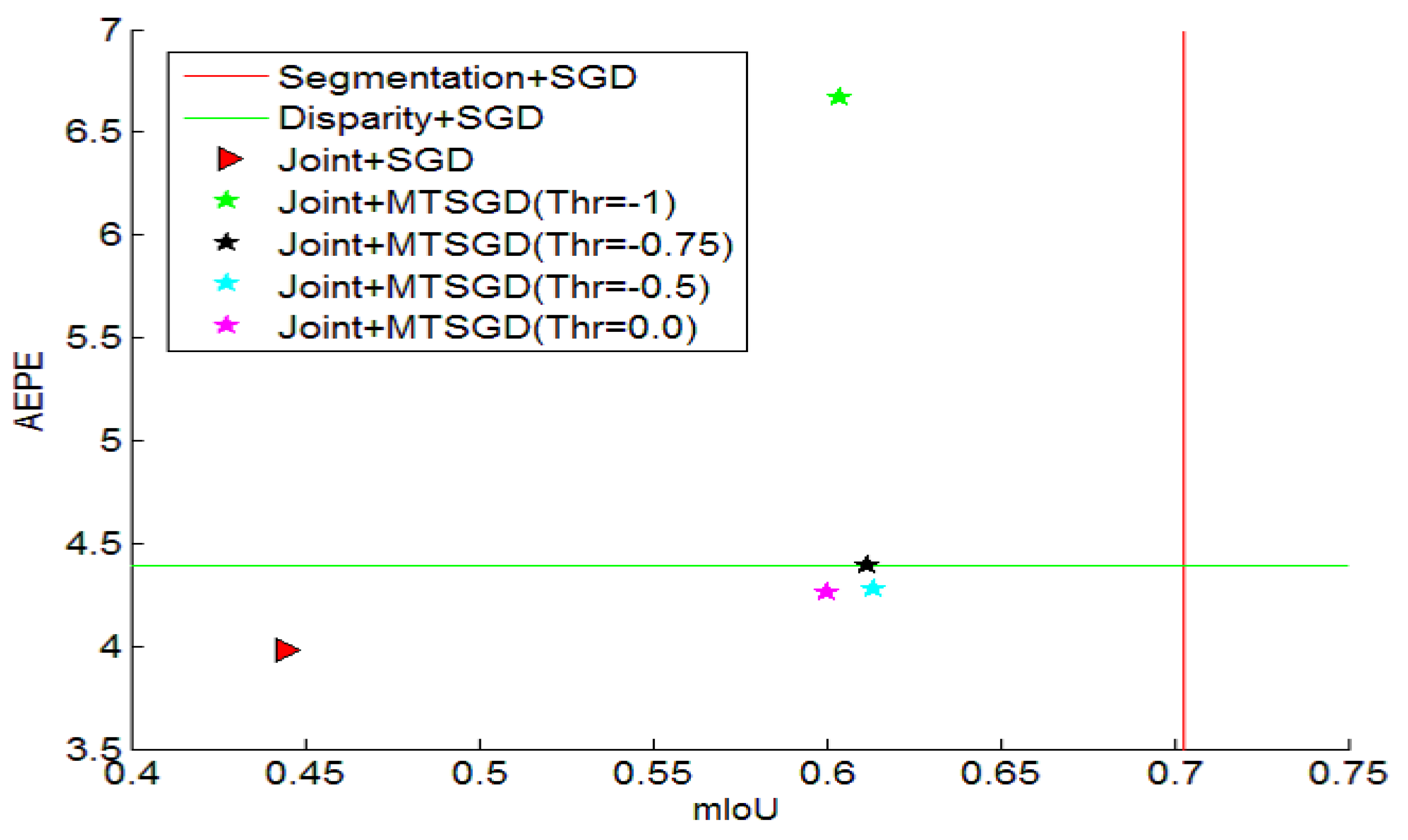
| Segmentaion + SGD | 1.0 | 0.0 | - | 70.3 | - |
| Disparity + SGD | 0.0 | 1.0 | - | - | 4.39 |
| Joint + SGD | 0.5 | 0.5 | - | 44.4 | 3.98 |
| Joint + MTSGD | 0.5 | 0.5 | −1.0 | 60.4 | 4.67 |
| Joint + MTSGD | 0.5 | 0.5 | −0.75 | 61.2 | 4.39 |
| Joint + MTSGD | 0.5 | 0.5 | −0.5 | 61.4 | 4.28 |
| Joint + MTSGD | 0.5 | 0.5 | 0.0 | 62.0 | 4.26 |
| Methods | Weight Decay | Threshold | Seg | Disp |
|---|---|---|---|---|
| (mIoU) | (AEPE) | |||
| MTSGD | 0.0 | −1.0 | 62.6 | 4.13 |
| MTSGD | 0.0 | −0.75 | 63.2 | 4.10 |
| MTSGD | 0.0 | −0.5 | 64.3 | 4.05 |
| MTSGD | 0.0 | 0.0 | 65.0 | 3.91 |
| MTSGD | 0.0001 | −1.0 | 60.4 | 4.67 |
| MTSGD | 0.0001 | −0.75 | 61.2 | 4.39 |
| MTSGD | 0.0001 | −0.5 | 61.4 | 4.28 |
| MTSGD | 0.0001 | 0.0 | 62.0 | 4.26 |
| Methods | Level | Threshold | Seg | Disp |
|---|---|---|---|---|
| (mIoU) | (AEPE) | |||
| MTSGD | channel | −1.0 | 60.4 | 4.67 |
| MTSGD | channel | −0.75 | 61.2 | 4.39 |
| MTSGD | channel | −0.5 | 61.4 | 4.28 |
| MTSGD | channel | 0.0 | 62.0 | 4.26 |
| MTSGD | filter | −1.0 | 59.7 | 5.32 |
| MTSGD | filter | −0.75 | 59.8 | 5.27 |
| MTSGD | filter | −0.5 | 60.0 | 5.12 |
| MTSGD | filter | 0.0 | 60.4 | 4.98 |
Publisher’s Note: MDPI stays neutral with regard to jurisdictional claims in published maps and institutional affiliations. |
© 2022 by the authors. Licensee MDPI, Basel, Switzerland. This article is an open access article distributed under the terms and conditions of the Creative Commons Attribution (CC BY) license (https://creativecommons.org/licenses/by/4.0/).
Share and Cite
Guo, Y.; Wei, C. Multi-Task Learning Using Gradient Balance and Clipping with an Application in Joint Disparity Estimation and Semantic Segmentation. Electronics 2022, 11, 1217. https://doi.org/10.3390/electronics11081217
Guo Y, Wei C. Multi-Task Learning Using Gradient Balance and Clipping with an Application in Joint Disparity Estimation and Semantic Segmentation. Electronics. 2022; 11(8):1217. https://doi.org/10.3390/electronics11081217
Chicago/Turabian StyleGuo, Yiyou, and Chao Wei. 2022. "Multi-Task Learning Using Gradient Balance and Clipping with an Application in Joint Disparity Estimation and Semantic Segmentation" Electronics 11, no. 8: 1217. https://doi.org/10.3390/electronics11081217
APA StyleGuo, Y., & Wei, C. (2022). Multi-Task Learning Using Gradient Balance and Clipping with an Application in Joint Disparity Estimation and Semantic Segmentation. Electronics, 11(8), 1217. https://doi.org/10.3390/electronics11081217