1. Introduction
Nowadays, the adoption of Unmanned Aerial Vehicles (UAVs), commonly known as drones, is experiencing a significant growth [
1], providing a plethora of benefits to our society. One of the main reasons for their popularity is their low cost, which has made it easier for the general population to acquire these electronic devices. Due to this growth, many companies have decided to make an economic effort to carry out research on UAVs in order to satisfy an unmet need, or to improve the performance of their main applications. Currently, apart from being a form of entertainment for the public, the use of these aircraft together, conforming a swarm, has made it possible to carry out more complex tasks [
2]. Among the most popular applications that we can highlight, we have: the control of agricultural crops, the monitoring of traffic, and the search for missing persons in the wilderness [
3].
For the tasks mentioned above, it is essential that drones work together, forming a swarm with sufficient autonomy to make decisions on their own, without the need for a human to control them. This intelligence allows a mission to be carried out in the most efficient way possible since, in the event that one of the drones breaks down, the swarm would reorganize itself to carry out its mission with minor disturbance [
4,
5].
Currently, despite the multiple investigations regarding drone swarms, there are still considerable problems in their monitoring that prevent their extended use. One of the main existing problems is the take-off of these drones [
6]. When trying to manage a swarm with a large number of aircraft, it becomes very complex to control that there are no collisions between them.
If we look into related literature, we find that few works in this area can actually be found. In fact, there is still some uncertainty regarding what exact procedures to use. As far as the take-off phase is concerned, there are basically two modes: sequential and simultaneous. Although the first method is quite effective at avoiding collisions, it introduces a very high total time; on the contrary, the second method is extremely fast, but quite prone to collisions. Hence, efforts in this area face the challenge of obtaining a protocol that allows preventing any mishap during take-off while achieving high time efficiency.
Fabra et al. [
7] proposed a heuristic that offers an efficient solution for the position assignment problem of a swarm. With this mechanism, each terrestrial location was assigned an aerial position, which obtained a nearly optimal total displacement distance. Although applying such a heuristic does not guarantee collision avoidance, such a solution provides greater safety, and reduces take-off time compared to a random approach (without any specific criteria).
In order to further optimize the assignment problem, Hernández et al. [
8] proposed a new take-off scheme based on the Kuhn-Munkres Algorithm (KMA) consisting of the application of graph theory. After the implementation of his proposal, it was possible to offer the optimal solution regarding the total displacement distance that the swarm has to exert. Despite achieving better results than the previous algorithm, it is still not enough to avoid conflicts in the flight paths during take-off.
In this paper, we present some novel algorithms for swarms composed of Vertical take off and landing (VTOL) UAVs; these algorithms are capable of optimizing the time elapsed in the take-off stage, while avoiding any collision. To this end, we will initially rely on the KMA [
9] to determine which UAV should go in each aerial location, as this algorithm is able to obtain the optimal solution in terms of flight distance [
8], which indirectly promotes having fewer collision chances during take-off. Having the position assignments as input data, we will be able to determine which multicopters collide with others and, to prevent this, we will form a list of groups of drones (batches) in which it is guaranteed that all the drones belonging to one of these groups can take off simultaneously, and without experiencing any conflict.
To validate the proposed algorithms, we carry out an exhaustive analysis of the performance achieved regarding the computation overhead and collision avoidance effectiveness of these algorithms. Moreover, a comparison of the results obtained with different position assignment algorithms will be made, thus allowing to determine which of them offers a higher performance. Different simulations will be carried out using different criteria to verify that the developed algorithm is, among other things, scalable with the number of drones, and secure.
The rest of this paper is organized as follows: in
Section 2 we provide an overview of the different stages of the swarm take-off procedure.
Section 3 presents the different algorithms we propose for detecting possible conflicts in the UAV take-off trajectories.
Section 4 details how, based on the chosen algorithm, we can segregate UAVs into different batches, where all those belonging to a same batch can take-off simultaneously. Then, in
Section 5 we start by presenting our simulation framework, detailing how tests are designed, and which performance metrics are used. Afterwards, our experiments and results are presented and discussed. Finally,
Section 6 summarizes the main findings of this paper, and refers to future works.
2. Take-Off Stages for a VTOL Swarm
In this section, we will detail the different stages through which we are partitioning the take-off of a UAV swarm to guarantee a successful process. As stated earlier, our focus is solely on UAVs of the VTOL type, as the proposed algorithms have as a basic requirement that aircraft should be able to stay at fixed aerial positions while other aircraft wait for their turn.
Basically, our proposal is to split the take-off into the following stages: (i) node detection, where we detect the positions of all UAVs after them being randomly deployed on the ground; (ii) position assignment, where we assign each UAV a specific position in the air according to the chosen target formation; (iii) conflict detection, where we calculate the possible collisions based on the expected take-off trajectories; (iv) batch generation, where we group UAVs into batches to create groups of conflict-free UAVs; and, finally, (v) maneuver management, where the UAVs are moved towards the target position following a three-segment approach. These stages are graphically presented in
Figure 1. We now proceed to elaborate further upon each of these stages.
- (I)
Node detection
In an initial stage, UAVs turn themselves on, attempt to obtain a GPS fix, and start their communications system for exchanging data with other UAVs. This allows detecting how many UAVs are available, what their ground locations are, and possibly selecting a swarm leader to be in charge of centralizing decisions whenever a ground control station is not available to perform such tasks. In our particular implementation (see [
7] for more details), we chose as leader the UAV with the most central position on the ground; such aircraft will send a request message to retrieve the exact number of drones available. Each drone that participates in the flight must respond, also indicating its location on the ground.
- (II)
Position assignment
When a swarm flight is to take place, the administrator must define what type of air formation should be adopted by the different UAVs deployed. Based on that input, each multicopter in the swarm should be assigned an aerial position that it will have to reach after take-off. The usual criteria when performing this assignment is to minimize the flight distances, to keep the take-off time overhead low, and also to minimize the chances of collisions between UAVs. Yet, achieving this can be complex and time consuming.
In previous works, we have studied different alternatives for performing the position assignment under the assumption that paths are following straight lines. In [
7] a heuristic is proposed that allows calculating a near-optimal position assignment for UAVs creating swarms that introduces a very low computational overhead. Its benefits compared to a naive random assignment are made evident. That solution is improved in [
8], where the KMA is used to achieve the optimal solution regarding such assignment by guaranteeing the minimal distance between terrestrial and aerial locations.
- (III)
Collision detection
Once UAV positions in the aerial formation are assigned, the following step is to check if any of the flight paths that should be taken by the different UAVs have a conflict with each other. If this occurs, a simultaneous take-off of both UAVs involved would possibly result in a crash, and, hence, should be avoided.
In the current work, we address this specific problem by proposing different strategies that are able to detect possible conflicts between UAV take-off trajectories in the most efficient manner. Our goal is to detect all possible conflicts (minimizing failed detections), while also reducing the time involved in such calculations. Such algorithms are elaborated in
Section 3.
- (IV)
Batch generation
Once all possible conflicts are detected (if any), the next step is to group the UAVs into batches. Inside each batch, we place UAVs that do not collide with the other UAVs of that batch. We aim for a high degree of simultaneity during the take-off, which corresponds to a low number of batches (with many UAVs in each batch, if possible). In
Section 4, we present an algorithm that splits the UAVs in the minimal number of batches required. Small waiting times are introduced between the take-off of one batch and the next one to minimize delays while guaranteeing safety.
- (V)
Maneuver management
In order to safely move the UAVs from their start location towards their target location, we decided to split their flight into three straight-line segments. These segments are shown in
Figure 2. Initially, the UAV will take-off vertically until reaching safety altitude
; this will give it enough ground clearance. It then moves diagonally, following a straight line, until it reaches its target position in terms of XY coordinates (
); finally, the UAV moves upwards to safely fit in its final position, and avoid other UAVs that are static or moving diagonally.
It is worth pointing out that, for the two vertical sub-paths of the UAVs at the beginning and end of the maneuver, we exclude the existence of collision risks because the distance between UAVs, whether on the ground or in the air, will always be greater than the safety distance. Therefore, we only have to detect collisions when aircraft are moving diagonally, corresponding to the trajectory formed by the points and .
3. Proposed Conflict Detection Algorithms
In this section, we will describe in detail the two main proposed approaches to detect conflicts in the flight paths to be followed by the different UAVs of a same swarm during the take-off process. For the first algorithm, named collisionless swarm take-off heuristic (CSTH), we will present a baseline implementation, followed by two different improvements. Then we present an alternative solution based on euclidean geometry called Euclidean distance-based CSTH (ED_CSTH).
3.1. Collisionless Swarm Take-Off Heuristic (CSTH)
This baseline algorithm will allow us to define some basic concepts and, in turn, it will serve as a reference for the creation of the proposed optimizations. Basically, the algorithm consists of checking if, for a certain three-dimensional location of a drone, which may belong to any location along its trajectory, there is a risk of a possible collision with the rest of the members that make up the swarm. To accomplish this, we must obtain all the intermediate points that each drone passes through on its way to the target aerial position (). To obtain all these positions, we will determine the three-dimensional vector that joins its terrestrial (), and its aerial location. In this way, this vector will be the one indicating the actual direction that the drone is going to follow starting from . Once this vector is obtained, we must normalize it and then use it to obtain each of the intermediate locations that make up its trajectory. In particular, we add this normalized vector (or a scaled version) to , to obtain the consecutive coordinates joining points and at the desired granularity. To optimize this procedure, and avoid repeating unnecessarily, a list of normalized vectors of all the existing drones in the swarm is initialized in the constructor of the main class, with their respective identifier, which allows us to obtain it quickly.
Regarding the chosen level of granularity, notice that, if the normalized vector has a length of 1 m, and the destination location for a UAV is about 20 m high, we will obtain, at least, 20 intermediate positions (counting the initial and final ones), since every time we move we do so in a value of 1 m of longitude distributed among its three coordinates. In the event that we multiply the normalized vector by two, we would move twice as fast, obtaining half the number of points than in the previous case. Hence, we will refer to granularity as the value by which we multiply the normalized vector, and it will be of utmost importance to optimize the computational costs. In turn, granularity is an extremely delicate factor, since the higher its value, the greater the probability that conflicts remain undetected due to the greater jumps between consecutive positions. Thus, we must study what granularity level allows us to optimize the computation time while guaranteeing the safety of the take-off phase. In
Figure 3, we can see an example of intermediate locations in the trajectory that a drone must follow to reach its aerial destination. As can be seen in the image, the distance between two consecutive points will depend on the actual granularity value adopted.
We now proceed to describe in more detail the proposed implementation for our algorithm. Two inputs are required for its development: the first one is the output of the position assignment algorithm. The second one is the list with the identifiers of the drones used for assessing the existence of possible collisions. Notice that it is not necessary to include all the identifiers of the drones participating in the flight, as explained later on.
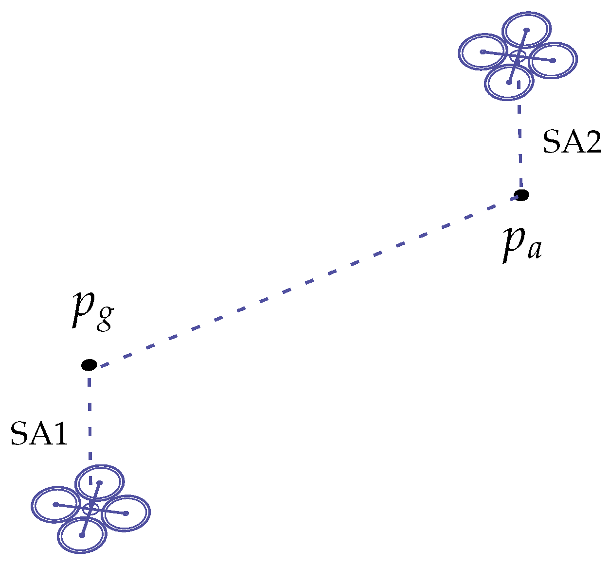
Focusing on the proposed algorithm, we will initially go through each of the identifiers belonging to the list mentioned in the previous paragraph. Then, for each drone, we will extract its three-dimensional
and
, along with its respective normalization vector. From these data, we will compare the distance of each of the intermediate positions located in the trajectory of the target drone with all the existing positions of the rest of the members of the swarm.
Figure 4 illustrates how the comparison between locations of pairs of drones is made.
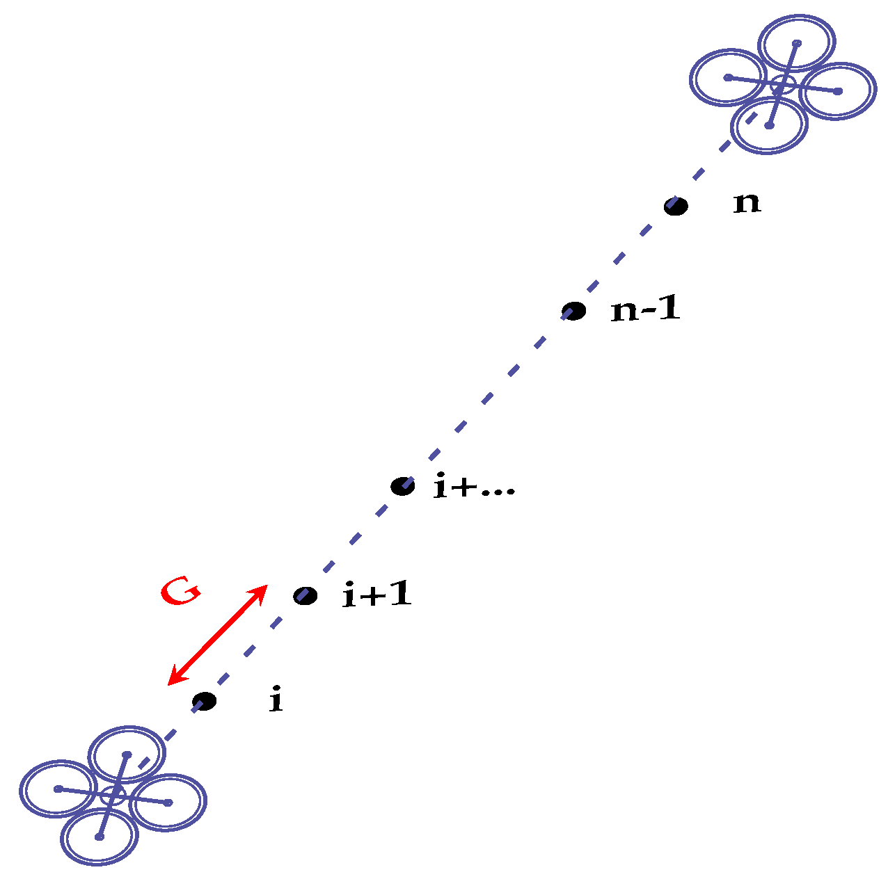
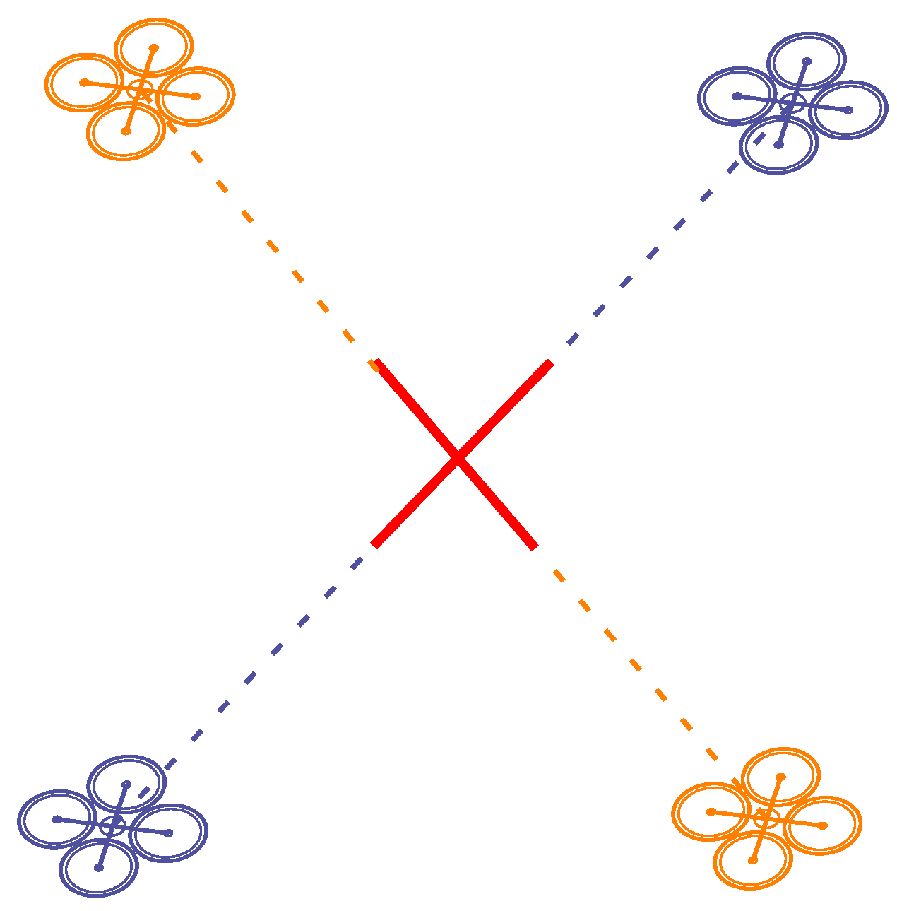
In these comparisons, if the distance between two locations is smaller than the value of the GPS error margin that we assign in the class constructor, a collision is detected. Notice that, when a possible collision is detected, it is no longer necessary to compare further positions, and the same procedure would be carried out with the next identifier on the initial list. In
Figure 5 we can see an example that shows the trajectory of two UAVs, and where the collision danger zone is represented with two red lines.
An important detail to emphasize upon is that, if no collision has been found for a specific UAV, it will not be part of future collision checks, since previously it had already been confirmed that there was no possible collision.
When there are no more identifiers in the list that we are going through, the algorithm will return all the potential collisions that have been detected. Algorithm 1 details how all the steps discussed above have been implemented.
| Algorithm 1 detectCollisionCSTH(uavs) |
- Require:
- 1:
for uavId in uavs do - 2:
uncheckedUAV.remove(uavId) - 3:
position = placement.get(uavId) - 4:
air = placement.getAir(uavId) - 5:
while position.distance3D(air) > granularity do - 6:
position = displace(position) - 7:
for nextUAV in uncheckedUAV do - 8:
nextpos = placement.get(nextUAV) - 9:
nextair = placement.getAir(uavId) - 10:
while nextpos.distance3D(nextair) > granularity do - 11:
nextpos = displace(nextpos) - 12:
if position.distance3D(nextpos) <= safetyDist then - 13:
collisionList.add(uavId) - 14:
goToLine(1) - 15:
end if - 16:
end while - 17:
end for - 18:
end while - 19:
end for - 20:
return collisionList
|
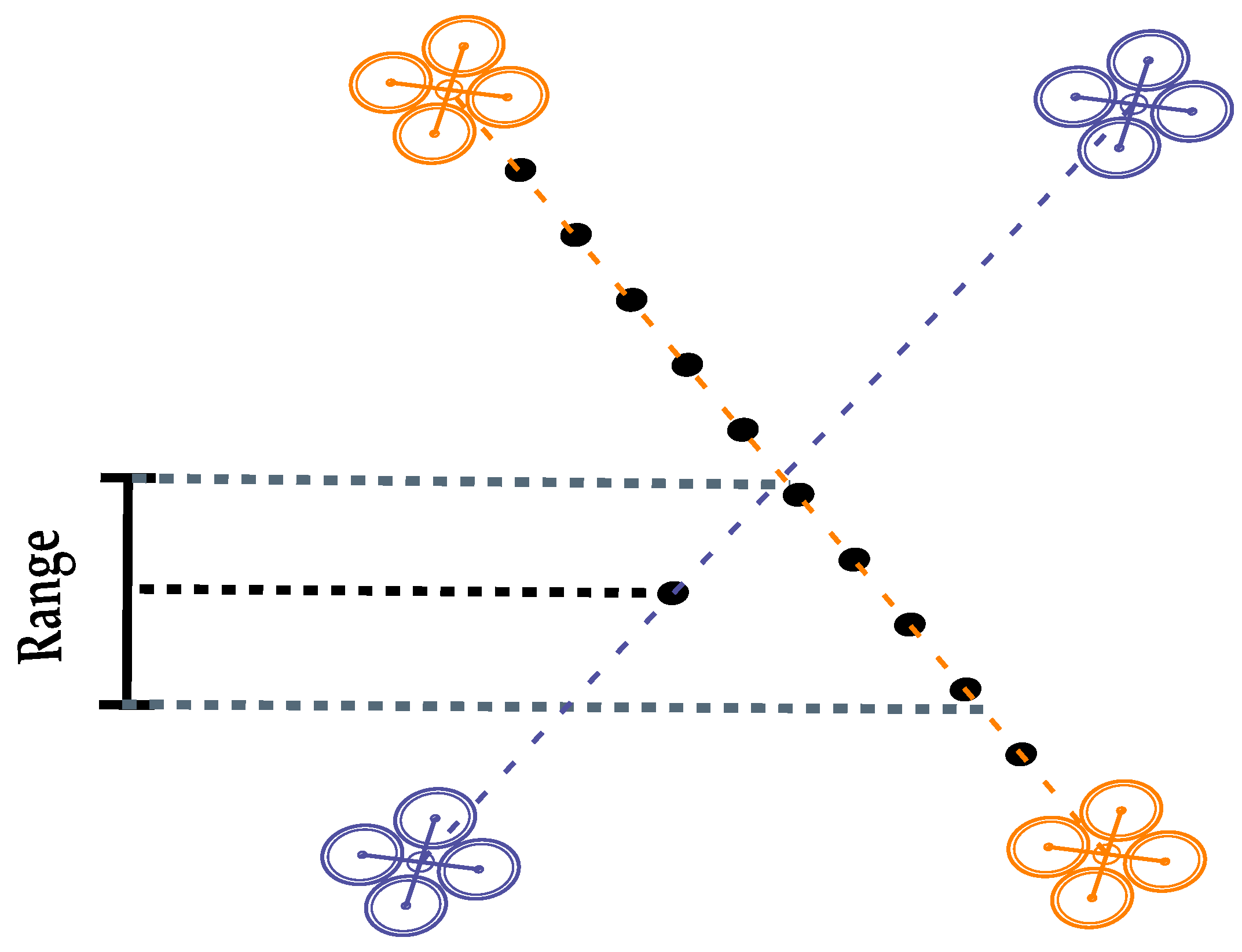
3.1.1. Optimization #1: Restricted Search Range (RSR)
In this first optimization, we improve the calculation time by reducing the number of points used for checking the security distance between two multicopters. To achieve it, instead of comparing each intermediate position of the current drone against all possible locations of the drones participating in the swarm, only a certain range of values will be considered; in particular, we will take as a central point the height of the position of the current aircraft, and so those positions whose heights are significantly different can be discarded. This way we can significantly reduce the computational cost of the algorithm without loss of accuracy. Notice that, to make this solution feasible, the user should input a double value that allows deriving the true limits of the range to be used. As an example, suppose a drone is at a location whose height is 10 m, and the value of the input parameter to construct the interval is of 2 m. With these data, our range would correspond to all those intermediate positions between 8 and 12 m. Once the limits of the interval are established, we would discard from the comparison all positions that remain outside this range.
In
Figure 6, we can visualize the operation of the CSTH+RSR algorithm. As can be seen, an intermediate position of the first drone is compared with only four positions for the second one, thus reducing the number of calculations to be performed. Like the previous version, the input value that we associate to the conflict range will be crucial to guarantee the detection of collisions since, if a low value is used, several possible conflicts could remain undetected. For this reason, we must carry out an exhaustive study of the different values that we can use to define our interval, and in this way ensure the reliability of our algorithm.
Going deeper into how this optimization works, the list with the identifiers of all the drones participating in the swarm mission is traversed in the same way as in the first version. It is worth mentioning that, for each of the intermediate points along the path of the drone under analysis, we obtain the value of its Z coordinate (equivalent to its height). To this value, we will add and subtract the value of the range parameter that the user has previously assigned to obtain the minimum and maximum values of our search interval. Here, we have to take into account that the minimum and maximum values of the interval must be equal to or less than the point
, and greater than or equal to the height at which its diagonal displacement begins. Once the height range is set, we compare locations with a height within this range of values. Lastly, the system used to check for collisions will be the same as the one discussed in its initial version. Similarly to the previous version, Algorithm 2 shows the changes made to implement this optimization.
| Algorithm 2 detectCollisionCSTH+RSR(uavs) |
- Require:
- 1:
for uavId in uavs do - 2:
uncheckedUAV.remove(uavId) - 3:
position = placement.get(uavId) - 4:
air = placement.getAir(uavId) - 5:
while position.distance3D(air) > granularity do - 6:
position = displace(position) - 7:
for nextUAV in uncheckedUAV do - 8:
nextpos = placement.get(nextUAV) - 9:
minz = min(minHeight,position.z - range) - 10:
maxz = max(maxHeight,position.z + range) - 11:
while nextpos.z <= maxz do - 12:
if nextpos.z <= minz then - 13:
nextpos = displace(nextpos) - 14:
continue - 15:
end if - 16:
if position.distance3D(nextpos) <= safetyDist then - 17:
collisionList.add(uavId) - 18:
goToLine(1) - 19:
end if - 20:
nextpos = displace(nextpos) - 21:
end while - 22:
end for - 23:
end while - 24:
end for - 25:
return collisionList
|
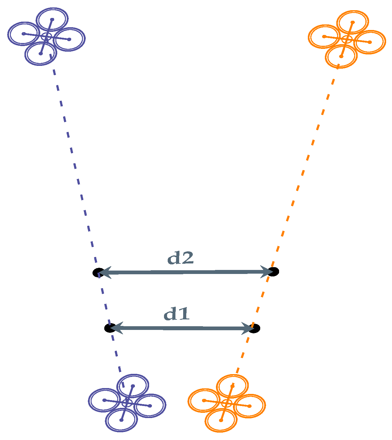
3.1.2. Optimization #2: Divergent Trajectory Detection (DTD)
This optimization seeks to reduce the computation cost of the initial version proposed by discarding those drones whose trajectory is distancing itself with respect to the current aircraft’s route, since the defined routes follow a straight line. This way, we can discard those lines that diverge from the line corresponding to the trajectory of the current drone. To implement this algorithm we will need to obtain, from the two aircraft whose paths are under comparison, their first two consecutive intermediate positions. We can then find two different situations depending on the values of the resulting distances.
Figure 7 shows the case where the second distance (d2) is less than the first one (d1), meaning that both trajectories tend to converge at some point (despite there is usually a separation between them in the 3D space). If this happens, we will proceed to the actual collision checking phase.
Conversely,
Figure 8 shows the case where the trajectories of both drones move apart as they move upwards towards their destination. In this situation, we can safely rule out that there is any danger of collision between the two compared drones.
As in previous sections, Algorithms 3 and 4 present the pseudocode relative to the improvements introduced in this section.
| Algorithm 3 detectCollisionCSTH+DTD(uavs) |
- Require:
- 1:
for uavId in uavs do - 2:
uncheckedUAV.remove(uavId) - 3:
position = placement.get(uavId) - 4:
nextposition = displace(position) - 5:
possibleCollision = checkConvergingLines() - 6:
while position.distance3D(air) > granularity do - 7:
position = displace(position, uavId) - 8:
for nextUAV in possibleCollision do - 9:
nextpos = placement.get(nextUAV) - 10:
while nextpos.distance3D(nextair) > granularity do - 11:
nextpos = displace(nextpos) - 12:
if position.distance3D(nextpos) <= safetyDist then - 13:
collisionList.add(uavId) - 14:
goToLine(1) - 15:
end if - 16:
end while - 17:
end for - 18:
end while - 19:
end for - 20:
return collisionList
|
| Algorithm 4 checkConvergingLines(position, nextposition, uncheckedUAV) |
- 1:
for uavId in uncheckedUAV do - 2:
pos = placement.get(uavId) - 3:
nextpos = displace(pos) - 4:
locationAux = displace(nextpos) - 5:
locationAux2 = displace(nextposition) - 6:
d1 = position.distance3D(pos); - 7:
d2 = nextposition.distance3D(nextpos); - 8:
if d1 > d2 then - 9:
possibleCollision.add(uavId) - 10:
end if - 11:
end for - 12:
return possibleCollision
|
3.1.3. Final Combined Version: CSTH+RSR+DTD
The two optimizations explained in the previous sections are compatible with each other. Although in the first one the goal is to reduce the number of comparisons between two UAV trajectories, the second one has the purpose of quickly discarding aircraft that will never collide (due to the diverging paths).
That said, in Algorithm 5 we can see the pseudocode of the combined version. We first make a list with those UAVs whose trajectory is divergent with respect to the drone that is being examined in the first loop. Next, we determine a range of values from the height of the first intermediate position of the aircraft. Finally, we compare this position with the rest of the locations of the other drones that are within the range of values created. If a potential conflict is detected, the affected drones are stored in the collision list.
| Algorithm 5 detectCollisionCSTH+RSR+DTD (uavs) |
- Require:
- 1:
for uavId in uavs do - 2:
uncheckedUAV.remove(uavId) - 3:
position = placement.get(uavId) - 4:
nextposition = displace(position) - 5:
possibleCollision = checkConvergingLines() - 6:
while position.distance3D(air) > granularity do - 7:
position = displace(position) - 8:
for nextUAV in possibleCollision do - 9:
nextpos = placement.get(nextUAV) - 10:
minz = min(minHeight,position.z - range) - 11:
maxz = max(maxHeight,position.z + range) - 12:
while nextpos.z <= maxz do - 13:
if nextpos.z <= minz then - 14:
nextpos = displace(nextpos) - 15:
continue - 16:
end if - 17:
if position.distance3D(nextpos) <= safetyDist then - 18:
collisionList.add(uavId) - 19:
goToLine(1) - 20:
end if - 21:
nextpos = displace(nextpos) - 22:
end while - 23:
end for - 24:
end while - 25:
end for - 26:
return collisionList
|
3.2. Euclidean Distance-Based CSTH (ED_CSTH)
When testing the algorithm presented in the previous section, it became evident that there was a clear trade-off between granularity and conflict detection effectiveness. In general, a low granularity would be recommendable to make sure all conflicts are detected; yet, by reducing the granularity, we are increasing the number of positions against which to compare, and this causes a considerable increase in the computational cost of the algorithm.
Hence, the proposal presented in this section is based on directly determining the Euclidean distance between the two UAV flight trajectories in the three-dimensional space. Similarly to the previous algorithm, a basic requirement for this new algorithm is that the trajectories of the drones during take-off follow straight lines. Thus, we can proceed to determine the distance between both lines in three-dimensional space using Euclidean methods.
The easiest case is checking whether the trajectories of two drones are parallel. Here, we would only verify that the vectors of each of the drones point in the same direction, that is, that their three coordinates are exactly the same. Although it is the least likely case, in such a situation we would confirm that there is no danger of collision between said drones as long as the distance between lines exceeds the safety threshold.
For the remaining cases, which are the most typical, we use the following formula to calculate the minimum distance between two three-dimensional lines:
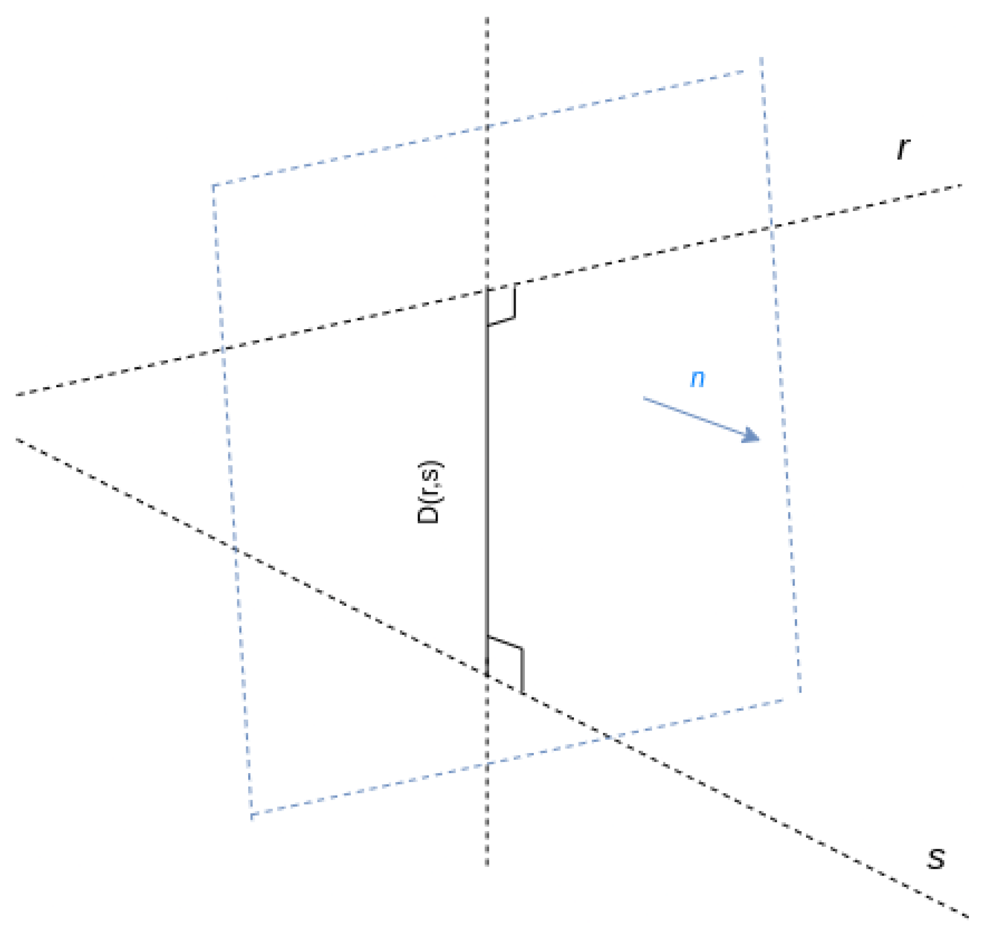
In this formula, the two lines in the 3D space are represented by letters r and s, while P would refer to a point on the line r () and Q to another point on the line s (). In the numerator we must calculate the determinant composed of the two vectors of the two lines, and the vector defined through points P and Q. Notice that in the denominator we will determine the cross product of the vectors of both lines. Once both values are obtained, we will divide them to obtain the minimum distance between both lines.
Once this distance is obtained, we must find out what are the coordinates of the points of each of the lines that belong to the minimum distance found. We do this to check if both points are within the height interval whose bounds are zero (ground level) and the height at which the swarm must fly (assuming formations on a same plane). Our proposal is to create a line that is perpendicular to the lines of each of the UAVs under comparison. This way, the points found on each of the lines are the ones that actually achieve the minimum distance between them.
Figure 9 shows the new line segment representing the minimum distance between lines
r and
s.
To obtain the required points, we need to perform a set of operations. First, we create the equations of the lines formed by the trajectories of the two UAVs we are comparing. After this, the distance between them will be determined as follows:
The letters
p refer to the points where the UAVs start the diagonal displacement, while the letters
d belong to their normalized vectors. In each of these equations, we find an unknown, symbolized by the letter
t. Second, we obtain the vector perpendicular to both lines by taking the cross product of the vectors of the two lines:
Then, we carry out the cross product between each of the vectors of the lines with respect to the vector obtained in the previous step. In this way, we create a plane that is perpendicular to both lines.
Therefore, the intersecting point
c1 of Line 1 with the above-mentioned plane, which is also the point on Line 1 that is nearest to Line 2, is given by Equation (
5). The point (
c2) on Line 2 nearest to Line 1 is calculated similarly.
Now, we need to check if this minimum distance is within the range set by the height. First of all, we will compare the resulting value with the safety distance that has been established. If the minimum distance is greater than the safety margin, we confirm that there is no conflict between these UAVs. In the opposite case, we can find three different cases:
If the coordinates of both points are within the height range of the aircraft, we confirm that there is a collision;
If both points are outside this range, we will say that there is no collision because both on and at the swarm height we make sure that there is a distance between UAVs that is already greater than the safety distance;
If one of the two points is within the range, and the other is not (either below the , or above the aircraft’s ), the point outside the range will be replaced by the nearest point within range. We then check the distance between both points, and if we obtain a value slightly less than the GPS margin of error, we consider that there is a collision.
The detection algorithm previously detailed is presented in Algorithm 6.
| Algorithm 6 detectCollisionED_CSTH(uavs) |
- Require:
- 1:
for uavId in uavs do - 2:
uncheckedUAV.remove(uavId) - 3:
for nextUAV in uncheckedUAV do - 4:
position = placement.get(uavId) - 5:
pos = placement.get(nextUAV) - 6:
if checkParallelVector(position,pos) then - 7:
collisionFlag = false - 8:
end if - 9:
if checkPathUAV(position,pos) then - 10:
collisionFlag = checkIntersectionPoint(position,pos) - 11:
else - 12:
collisionFlag = checkDistMin(position,pos) - 13:
end if - 14:
if collisionFlag then - 15:
collisionList.add(uavId) - 16:
goToLine(1) - 17:
end if - 18:
end for - 19:
end for - 20:
return collisionList
|
4. Batch Generation Strategy
In the previous chapter, we have presented different algorithms that are able to detect potential collisions between UAVs. These algorithms return a list of UAV with conflicting take-off trajectories.
The goal of this chapter is, based on such conflict list, to propose an algorithm that allows us to separate the UAVs into batches. In this way, aircraft belonging to a same batch should be allowed to take off simultaneously, without any conflict between their trajectories.
First of all, it is very important to take into account that the batches of drones that are to be launched first should correspond to the drones travelling greater distances. The solution that has been used in the present work is to modify the collision detection algorithm so that, instead of going through the list of UAV identifiers that we obtain as input data, it previously orders that list according to travel distance per UAV. Hence, after assigning UAVs to different batches, all we have to do is order them by their average distance.
Going deeper into the proposed algorithm, three input data are required for its correct implementation. The first one is the list of collisions obtained in the collision detection algorithm. The second one is the list of UAV identifiers. Additionally, the third one is the list of previously formed multicopter batches (during its first call, it will be empty). This last list plays a very important role since, being a recursive method, this variable will be in charge of storing the result of the batches made in the first iterations of the method.
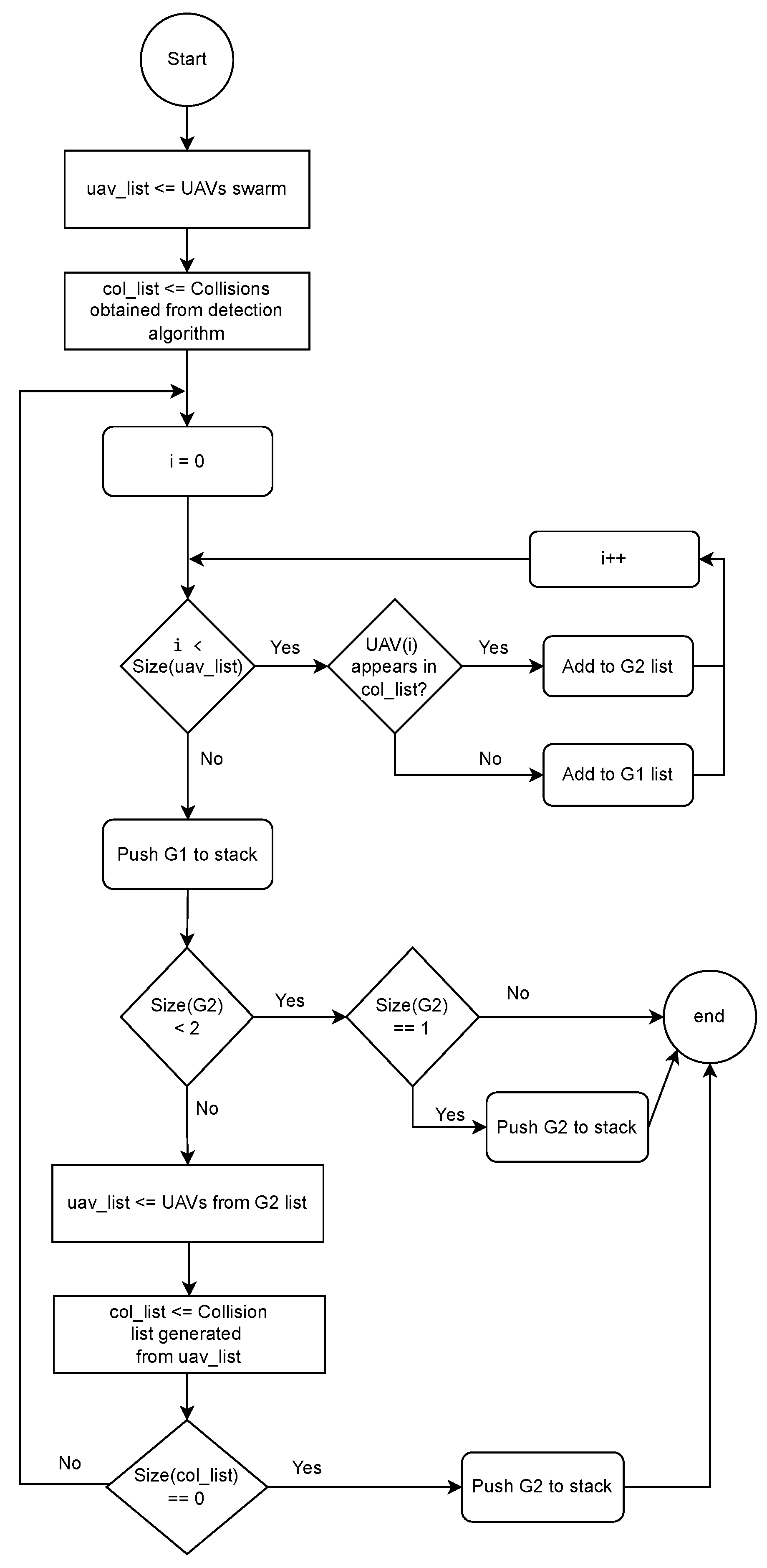
In
Figure 10, we visualize the operating diagram of the mechanism for generating batches. For each UAV belonging to the list of swarm identifiers, we check if it appears in the list of collisions that we obtain as a result after applying the collision detection mechanism. If we observe that it belongs to the list, we will directly insert it into a new group (G2) where those drones that do not comply with the safety distance will temporarily be stored. Otherwise, if an UAV does not appear in said list of collisions, it will join group G1. This way, we manage to divide all the existing identifiers in the swarm into two subgroups, differentiated those aircraft that meet the flight safety distance requirements, and those that do not.
Then, we add the labels of the UAVs that are part of G1 as a new batch to the output data, as they do not generate any conflict between them and, therefore, they will be able to take off simultaneously without causing any risk. After that, the next step that we must carry out will be to check the number of existing labels in G2. If its quantity is less than two, we enter the base case of the recursive method. Here, we check whether G2 is empty or not. In case it is not empty, we will add a new batch with its identifier, and the algorithm will thus end. If G2 is empty, we will directly return the final result of the algorithm.
Afterwards, if the number of G2 identifiers is greater than or equal to two, we would proceed to create a new list of drones with only the labels belonging to G2. From the identifiers in this list, we will search for existing collisions with each other. If this collision list is empty, we will insert the tags of the G2 UAVs into a new batch, and return the result of the algorithm. If it is not empty, we will restart the procedure from the beginning except that, this time, both the list of UAVs and collisions will be different from the first iteration. Furthermore, we will empty G1 and G2 so that they can be filled with the new identifiers. This corresponds to the recursive case whereby we return to the starting point, but now having a reduced dataset.
Figure 11 shows an example of the batch generation mechanism in a swarm composed of four aircraft. Using our collision detection algorithm, we obtained the information that there is a possible risk of collision between the first and the second UAV, as well as between the third and the fourth UAVs. We start the batch process with UAV 1. Since there is a risk of collision, UAV 1 is placed in batch B. We continue with UAV 2, this UAV has no risk of collision (we already solved the collision with UAV 1). Therefore, it is placed in batch A. Next is UAV 3; this UAV collides with UAV 4 and, therefore, it is placed in batch B. Finally, UAV 4 has no risk of collision, hence it is placed in batch A. This ends the first iteration of the batch process. We start the second iteration of the batch process, here we go over all the UAVs in batch B and confirm that they do not collide. Since UAV 1 and UAV 3 do not collide, we do not have to create additional batches, and we end the batch process.
5. Results
In this section, a wide set of simulations will be carried out to assess the performance of the various collision detection algorithms proposed, and to verify that the take-off stage is carried out safely. First, we will explain our simulation setup. Then, in the first set of experiments, we will determine the ideal granularity for the CSTH-based algorithms. Then, we will determine their computational overhead. The best performing CSTH variant is then compared against the ED_CSTH algorithm. Finally, we will measure the overall take-off time for the best possible case achieved.
5.1. Simulation Setup
To determine whether the goals of this work have been accomplished, it is necessary to carry out multiple tests in a simulation environment with which to verify the absence of collisions before carrying out experiments on real drones. This phase is one of the most important ones in any project aimed at drone swarms, since hasty management could mean the loss of a large amount of time and money in the event that these aircraft suffer some type of accident. In this work, we have used ArduSim [
10], as it is a real-time flight simulator based on Software-in-the-Loop UAV emulation that allows us to simulate missions with a considerable number of drones (more than 500), and it also offers us great precision in the data collected. This simulator was developed in Java, and it is entirely open source [
11].
For our tests, we are going to compare the different proposed schemes by varying two variables: the number of UAVs conforming the swarm (for scalability analysis), and the swarm topology. Notice that, when taking off, UAVs usually take a random position on the ground, maintaining a small distance between them. Yet, when they are flying as a swarm, usually a mission-specific aerial formation is defined. In our simulation we will consider three different aerial formations: linear, circular, and matrix. In the case of the linear one, it is very useful in precision agriculture applications [
12] (among others) because they allow a larger area to be covered quickly, since the UAVs are placed forming an overhead line. The circular formation is characterized by having an aircraft in the middle, normally with the functionality of a coordinator, and the rest of the drones are placed around it forming a circular formation. Finally, we test with the matrix formation that, depending on the number of UAVs used in a given swarm, will try to organize them in a matrix of
n x n drones as much as possible; this is usually the most compact choice.
Table 1 shows the simulation parameters that we are going to use with their respective values. The safety parameter will have a value of 8 m, and it represents the GPS error margin of the UAVs. Then, the maximum height that it will be used in the air locations is 20 m, except for experiments
Section 5.5 and
Section 5.6, where that value is increased to 30 m instead.
Concerning our target performance metrics, we are going to assess the different algorithms presented based on the amount of undetected collision risks, computational time overhead when determining these potential risks, and the overall take-off time, which also accounts for other algorithms, including the batch generation strategy and the take-off strategy.
The machine used to collect the results presented in the next section has an Intel processor model i5-2500K, with four cores that provide a basic frequency of 3.30 GHz. As far as memory is concerned, its size is 4 GB (DDR3 type).
5.2. Experiment 1: Obtaining the Ideal Granularity
One of the main problems that we run into in the baseline CSTH algorithm, and its respective optimizations, is that we need to ensure that the granularity that we employ allows us to obtain all the areas of conflict when taking off a swarm of UAVs. As explained in the previous chapters, granularity is going to play an essential role when it comes to extracting all the intermediate positions of a drone between and . This means that the choice of the granularity value is going to be a critical process, since, if we select a high value, we could obtain three-dimensional locations whose distances are greater than the value assigned to the proposed GPS margin of error and, therefore, certain collisions could remain undetected.
Taking this problem into consideration, the main objective of this first set of simulations is to determine the granularity value that guarantees obtaining all the possible conflicts between the UAVs conforming the swarm. To do this, we vary the granularity value using a fixed number of drones, and for each of the three available aerial formations (circular, linear, matrix). The purpose of these tests is to examine and analyze the relationship between the number of undetected collisions and the chosen granularity value. As a starting point for the test, it has been decided to start with a granularity value equivalent to one meter, and increase it by one meter until reaching the value of 10. For these simulations, we use 200 drones so that the number of possible conflicts to be detected is significant enough to reach a conclusion. The safety distance that has been proposed in this experiment is of 8 m, so that the safety of the movement maneuvers carried out by the drones can be guaranteed despite GPS inaccuracies. It is also of great interest to mention that the minimum distance between aircraft ground positions is 10 m. Moreover, we will also define a (minimal) distance between the aerial locations of the swarm of 20 m. Finally, the flight altitude that we will use in these experiments is also of 20 m.
Figure 12 allows gaining insight on the trade-off between granularity and time overhead involved. As shown, calculation times are reduced considerably as we increase granularity values. It is important to note that, in this figure, the values shown are on a logarithmic scale because of the differences in calculation time between the three available formations; for 200 drones, such difference becomes really large and, using such a scale, we managed to improve readability. Based on these results, it becomes clear that there are great benefits in using high granularity values. However, as stated above, increasing the granularity is in conflict with collision detection accuracy.
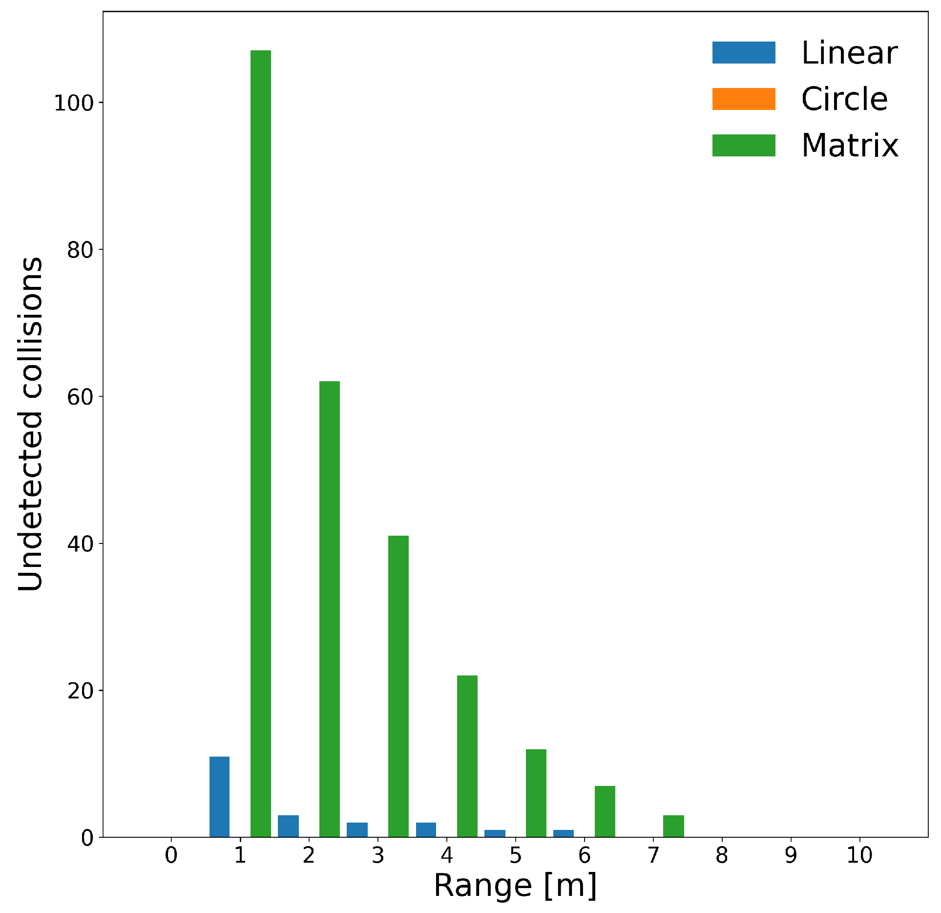
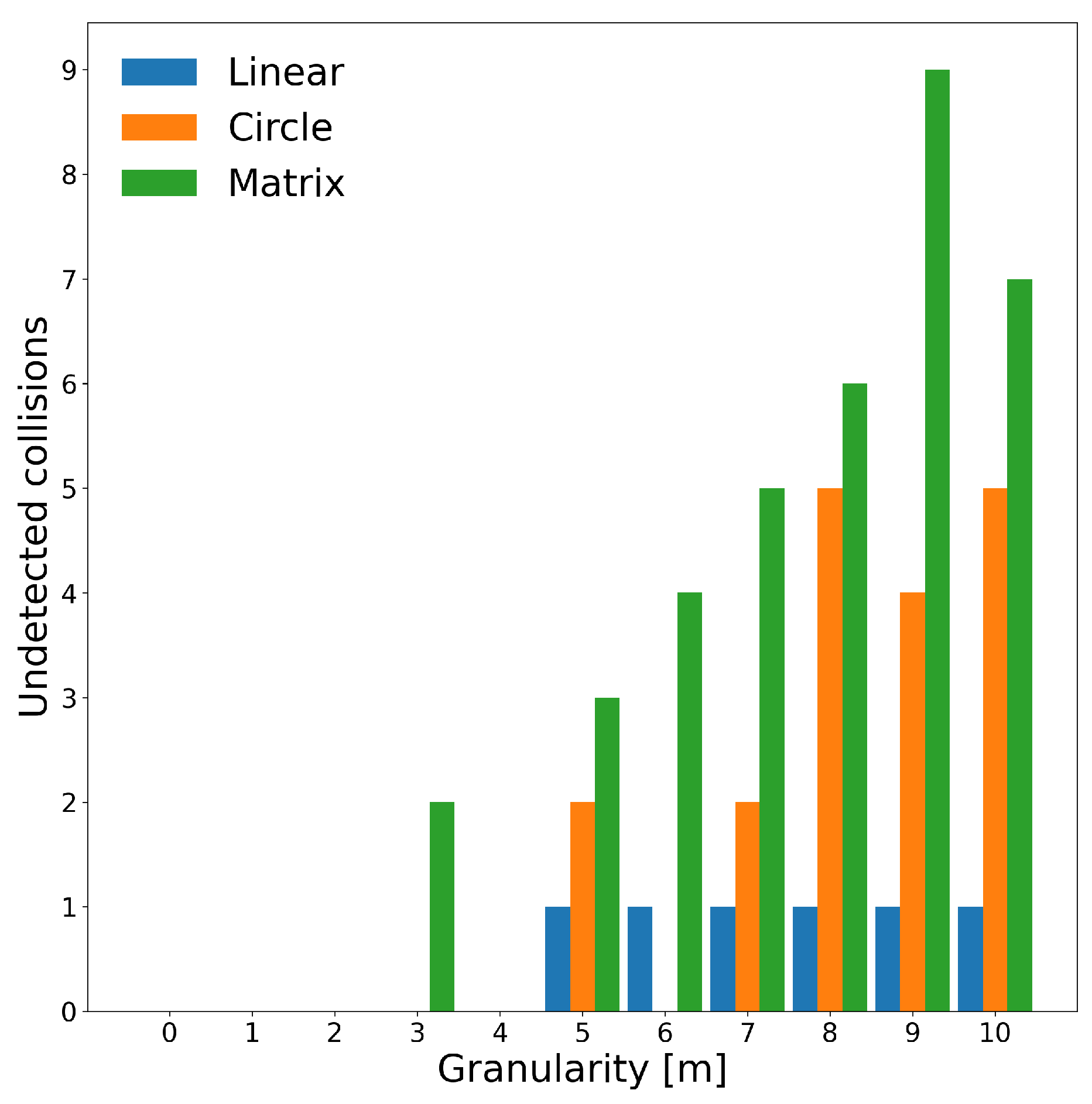
To gain further insight into such a problem,
Figure 13 shows the potential number of collisions that remain undetected as we increase the granularity value. This value is calculated as the difference between the number of collisions obtained from each of the simulation executed with respect to the first test (with granularity equal to one), which is our reference. As shown in the figure, for granularity values of 3 m and greater, we begin to miss the detection of some trajectory conflicts. If we continue to increase this value, we conclude that the missed conflicts reach high values, which prevent the take-off maneuver of the UAV swarm from being reliable. Hence, a granularity equal to two becomes the best choice, as it allows us to reduce the computational time overhead while still detecting all existing conflicts.
5.3. Experiment 2: Comparison of Computation Time between CSTH Algorithms
The purpose of this experiment is to evaluate the performance of the collision detection algorithms based on spatial discretization (CSTH family). To do this, we develop a set of tests with different numbers of UAVs for the available aerial formations.
Before starting, we need to set a value as input for the CTSH+RSR algorithm to derive the true limits of the range to use. As mentioned in the previous chapter, this optimization consists of discarding the intermediate positions whose height is outside the established interval.
The simulation parameters used in these tests are exactly the same as in the first experiment. In addition, to obtain the intermediate positions, the value of the granularity resulting from the previous experiment (2 m) has been used.
Figure 14 shows the results of the simulations we did to find a numerical value that allows us to establish a reasonable interval. To do this, we use a fixed number of UAVs equivalent to 200, so that the number of potential conflicts is significant. One of the most interesting details is that, for the circular formation, we detect all collisions regardless of the interval range used. However, for the remaining formations, we find that a large number of undetected collisions remain, especially in the matrix formation. In fact, for both the linear and matrix formations, we see a clear trend where, as we increase the range of values, more collisions are detected, until reaching a value where all collisions are detected. In our case, this is achieved for a range value of 8 m (equivalent to 16 m of difference between the lower and upper limits of the interval). Although for this particular experiment this value is very high due to the fact that the maximum height for the drones is set to only 20 m, it already represents a significant improvement with respect to the performance of the baseline CSTH algorithm.
We now proceed by carrying out a performance comparison in terms of calculation time. Nothing has been previously commented on the CSTH+DTD optimization and the combined version (CSTH+DTD+RSR), because no additional parameters are required for their execution.
To compare these algorithms, we have decided to carry out several simulations, varying both the number of drones and the formation used. This way, we can more clearly appreciate the difference between each of the versions. Additionally, notice that the simulation parameters used have been the same as in the previous experiments.
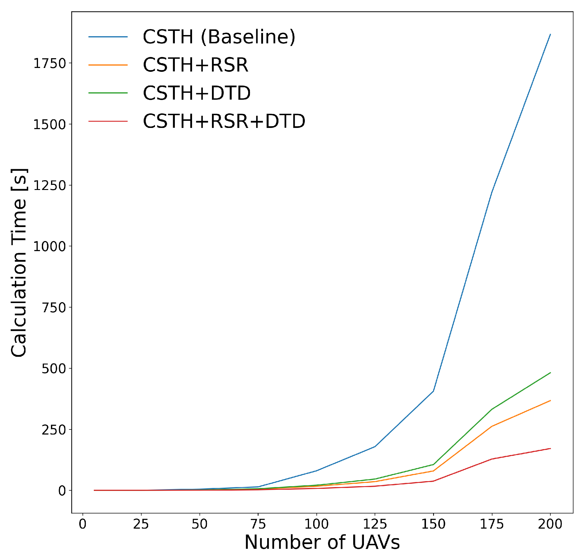
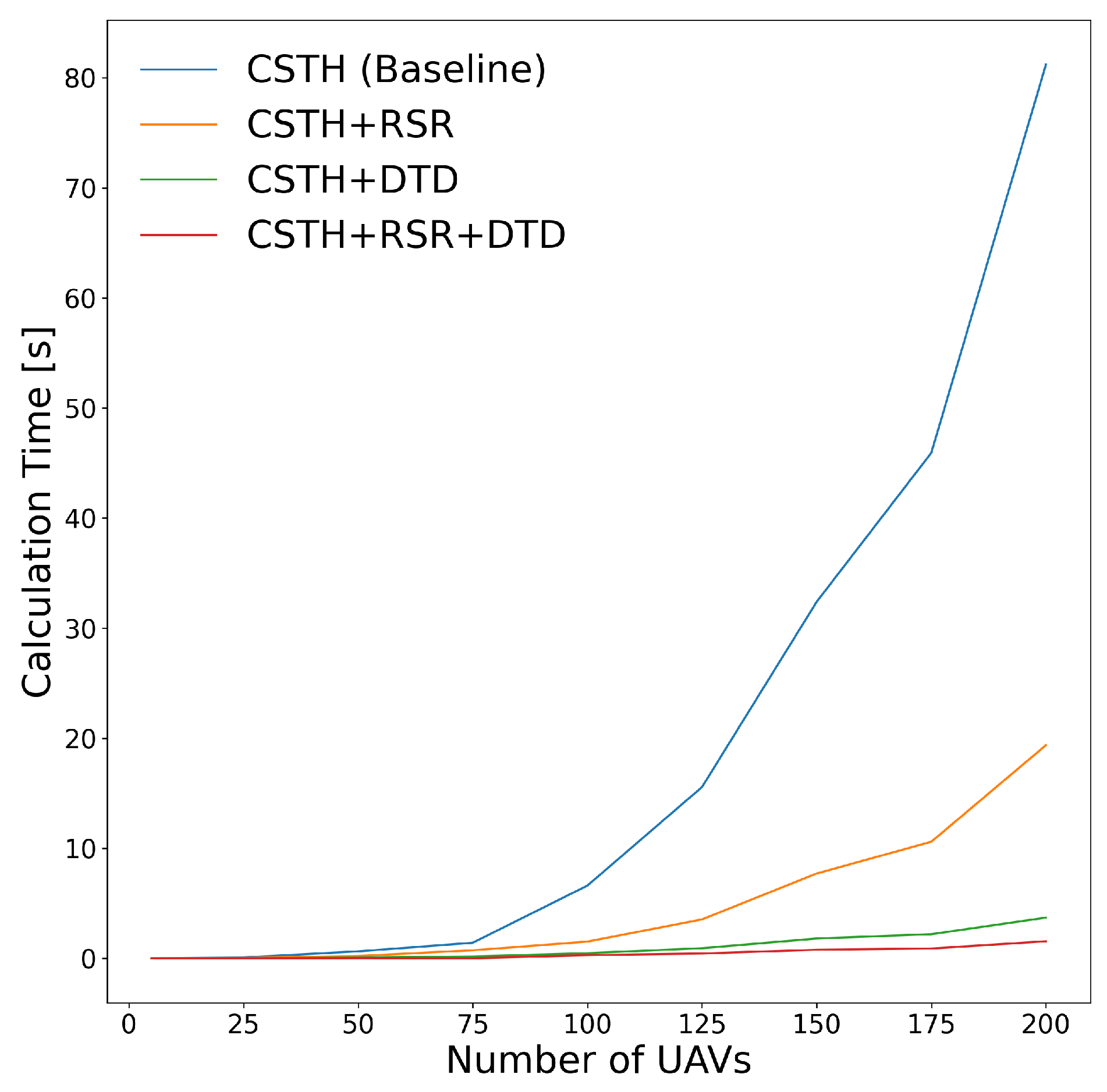
Figure 15 highlights that there is a clear difference between the different CSTH versions as we increase the number of drones. For up to 75 drones, there are almost no differences between the calculation times, obtaining a value of approximately one second. Beyond this number of aircraft, the differences begin to be significant. With a value of 200 drones, we can see that the CSTH Baseline algorithm introduces a delay of 81 s to guarantee collision detection, while in the CSTH version (RSR+DTD) the delay is merely 1.5 s. Regarding the CSTH+RSR algorithm, and for the same amount of drones mentioned in the previous test, we obtain a time of 19 s (4 times faster), while for CSTH+DTD we have a value of 4 s, equivalent to approximately 20 times higher efficiency.
The linear air formation is by far the one taking the most time to perform the algorithm calculations. This is due to the greater distances between the ground and aerial locations compared to other formations. That said,
Figure 16 shows the computation time for the different algorithms. Similarly to the previous case, from 75 drones onwards we observe clear differences between versions. Using the maximum number of UAVs, we see that the CSTH Baseline algorithm needs a total of 31 min to complete the collision detection procedure. This time it is prohibitive since, to the calculation time, we must add the take-off flight time of all the UAVs in the swarm. Once again, the combined version is the one with the best performance, allowing all collision danger zones to be detected in under 3 min (10 times more efficient). The CSTH+RSR optimization manages to detect all collisions in about 6 min (equivalent to about 5 times faster), while the CSTH+DTD algorithm does it in about 8 min (about 3/4 times more efficient).
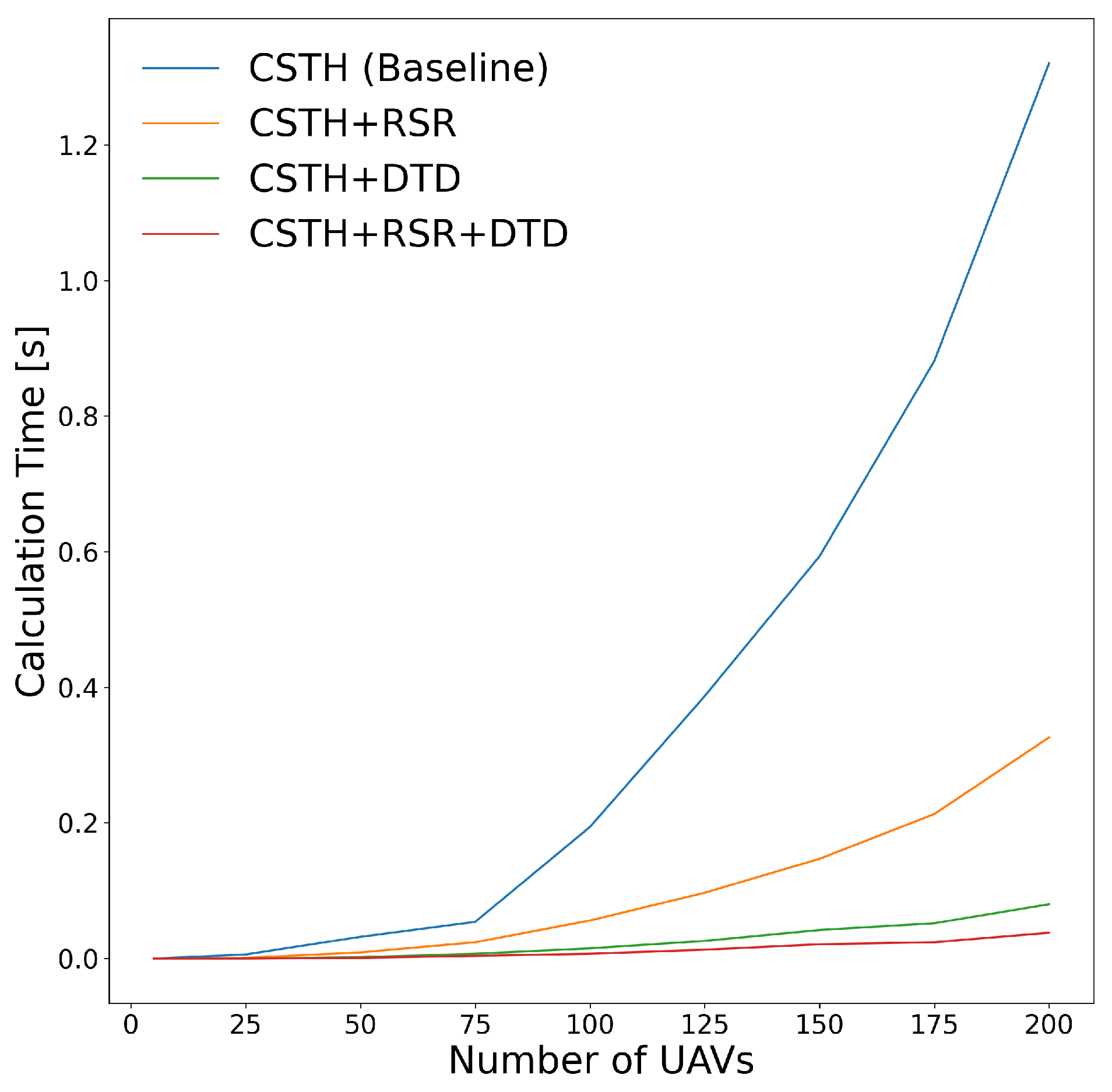
Lastly, and inversely to what happened in the linear formation, the time needed to calculate conflicts for the matrix formation is very low, since their aerial locations are usually closer to each other, meaning that take-off paths are more vertical. In
Figure 17, we visualize the differences in terms of calculation time for the proposed algorithms. Again, the CSTH algorithm is the one requiring more time (1.32 s) to obtain a solution with 200 aircraft, while the combined version again improves performance considerably, needing only 0.038 s. Finally, note that the CSTH+RSR optimization requires a time of 0.326 s, while the CSTH+DTD version performs it in about 0.08 s.
In summary, with the results obtained, we can affirm that the CSTH algorithm with both DTD and RSR optimizations is the most efficient version. This is because it achieves a considerably shorter calculation time than the other variants in all available air formations. In addition, in each of the tests carried out with a different number of drones, it detects the same number of possible collisions as the initial version, thus, ensuring the reliability of the algorithm.
5.4. Experiment 3: Comparison of Computation Time between CSTH and ED_CSTH Algorithms
In the two previous sections, we focused on finding the most efficient approach for the CSTH algorithm, which is achieved by combining both RSR and DTD optimizations. In this section, we proceed to compare such optimal solution against the alternative algorithm we propose, which is based on directly determining the minimum distance between two UAV trajectories using Euclidean geometry. Notice that these two algorithms are radically different in their approach, where the first one relies on many but simple calculations, while the second one requires few but more complex calculations.
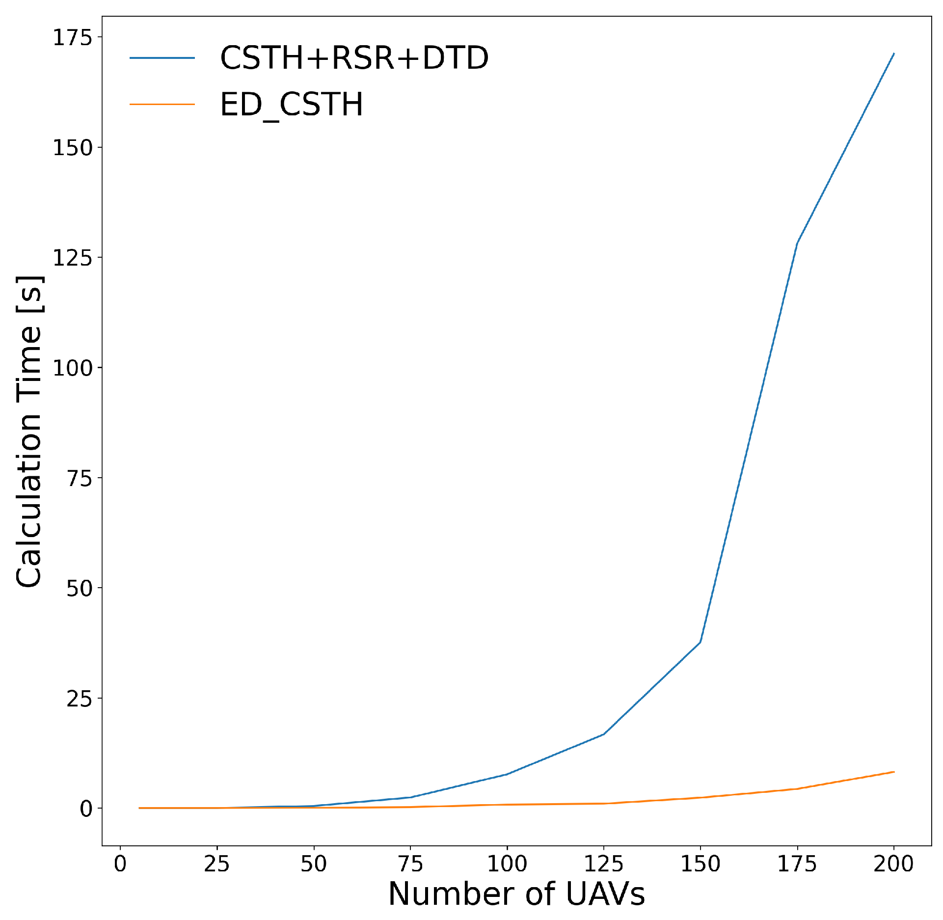
Figure 18 shows the calculation times for both algorithms when increasing the number of UAVs, and focusing on the circular formation. We observe that, with a quantity beyond 100 drones, the ED_CSTH algorithm increases its time with respect to the results obtained with the CSTH+RSR+DTD. In fact, when reaching 200 UAVs, the ED_CSTH algorithm takes 10 s to detect collisions while CSTH+RSR+DTD achieves it in 1.5 s. Hence, in this situation, the latter offers a clear performance advantage, being almost seven times faster.
Figure 19 presents the calculation time obtained for the linear formation instead. In said figure, we find the opposite situation compared to the circular formation. In fact, while the ED_CSTH algorithm manages to maintain a nearly constant calculation time regardless of the number of UAVs used, the CSTH+RSR+DTD algorithm suffers a significant penalty for experiments with a greater number of drones, providing a calculation time of almost 3 min.
Finally,
Figure 20 shows the calculation time for the matrix formation. In this case, the CSTH+RSR+DTD algorithm manages to perform all operations in hundredths of a second on any number of UAVs. On the other hand, the baseline CSTH algorithm less efficient, i.e., to obtain the results with 200 aircraft it takes almost 1.5 s.
As can be seen, for the circular and matrix formation we obtain that the combined version is faster and more efficient, while in linear formation the ED_CSTH algorithm achieves a better performance. In short, the conclusion that we draw from these figures is that, depending on the situation in which we find ourselves, it will be more useful for us to use one version or another. However, for the following simulations, it has been decided to use the ED_CSTH algorithm because its average time considering the three formations is lower.
5.5. Experiment 4: Comparison of the Take-Off Flight Time against the Sequential Procedure
Once we have chosen the detection algorithm to use, the next step is to obtain the take-off flight time of our proposal (named semi-simultaneous), and compare it against the sequential procedure. To determine the total time associated with the take-off in the semi-simultaneous approach, we must add the time from the assignment algorithm, the calculation time of the detection algorithm, and the take-off flying time of the UAVs swarm.
To carry out the respective tests, it is convenient to comment on the simulation parameters that have been decided to use. Firstly, it has been decided to carry out a total of seven simulations using different numbers of aircraft for each of the available air formations. Unlike previous experiments, the maximum number of drones used will be reduced from 200 to 150. Another change that has been made is related to the maximum height of aerial positions. Instead of having a height of 20 m, it has been decided to increase that figure to 30. As for the rest of the simulation parameters, they remain the same as in the previous experiments. Since on this occasion we have the ArduSim graphical interface to carry out the calculations, in the event of a risk of collision between two aircraft, its existence would be notified, and an emergency landing would be made. In the ArduSim log files, we can easily identify the UAVs that have caused the collision with their respective 3D locations and the distance between them.
Figure 21 shows the take-off flight times, expressed in minutes, of both procedures for each of the air formations. To perfectly distinguish the results obtained, the continuous lines will refer to the formations of the sequential algorithm, while the dashed lines will be to the semi-simultaneous one. Going deeper into the figure, we see that, in each of the simulations carried out with a different number of aircraft, the semi-simultaneous algorithm notably improves the performance obtained compared to the sequential one. Going into detail in each of the aerial formations, and for the specific case of launching 150 drones, we see that, in the matrix formation, we went from having a total time of 58 min to only 3.6 min. This big change is due to the fact that, for this type of formation, very few conflict zones are detected and, therefore, it is necessary to group the drones in a smaller number of batches. Another aspect that explains such a short take-off flight time is that this formation is the one that benefits the most from the use of the KMA assignment algorithm. This means that the total movement made by the UAVs, placed randomly on the ground, is considerably lower than that of the rest of the formations. In the case of the circular formation, the necessary 2.5 h are contrasted with the almost 17 min with a semi-sequential take-off. Here, we have a considerable number of potential collisions leading to the creation of a large number of drone batches. Finally, the linear formation is the one that takes the longest time, since the total distance that the swarm has to travel is more than a thousand times greater than the overall matrix formation distance. That said, from a total time of almost 4 h, it is possible to reduce it to 19 min. On this occasion, the vast majority of UAVs belonging to the swarm are in potential conflict zones because their trajectories are very similar; note that half of the drones will move to the left, while the other half will move to the right to form a line in the air. For this reason, the number of drone batches will be high, since in most situations in each batch there will be only two aircraft, whose directions are opposite. An important detail to comment on is that, for both the circular and the linear formation, having a high number of drone batches will multiply the effect of adding an additional waiting time (3.5 s) introduced between the take-off of each one of them.
5.6. Experiment 5: Study of the Results Obtained with the Different Assignment Algorithms
After analyzing the improvement obtained by the semi-simultaneous procedure versus the sequential procedure, this last study focuses on assessing the behavior of our proposal when using different positions allocation algorithms. In this experiment, an exhaustive comparison will be made of both the take-off flight time and the number of batches generated.
As already mentioned in the previous chapters, to define the position that each UAV must occupy in the air, we have used the KMA assignment mechanism. This scheme provides an optimal solution in terms of the total distance travelled by UAVs to reach their aerial locations. In this way, by making use of said assignment, it would be ruled out that several aircraft would have to fly to another end of the swarm, causing the number of conflict zones to increase significantly. However, there is uncertainty whether an optimum in terms of flight distances necessarily represents also an optimum in terms of the number of batches generated, and, thereby, the overall take-off time.
Hence, for these experiments, we will perform the initial position assignment with both KMA and our heuristic method proposed in [
7]. As discussed earlier, this heuristic provides a slightly suboptimal solution after being tested in regular air formations, but is faster in executing computational calculations compared to KMA.
To obtain the data with this new allocation algorithm, we are going to use the same simulation parameters used in the previous experiment in order to be able to reuse them.
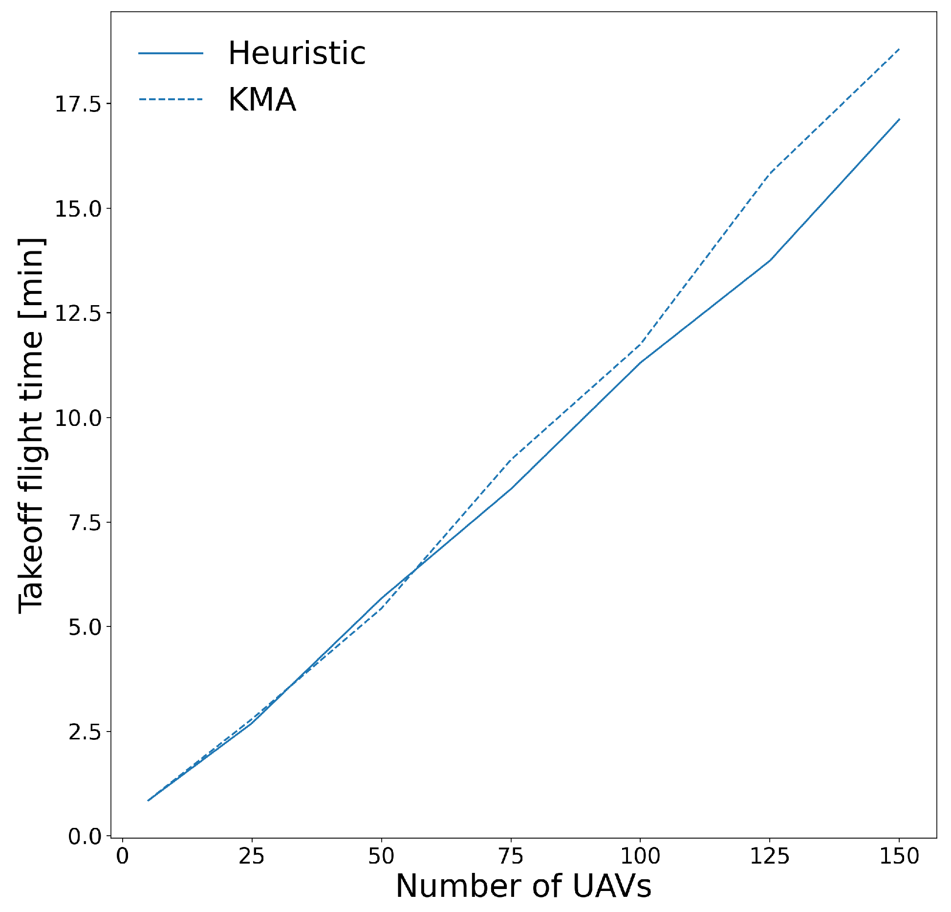
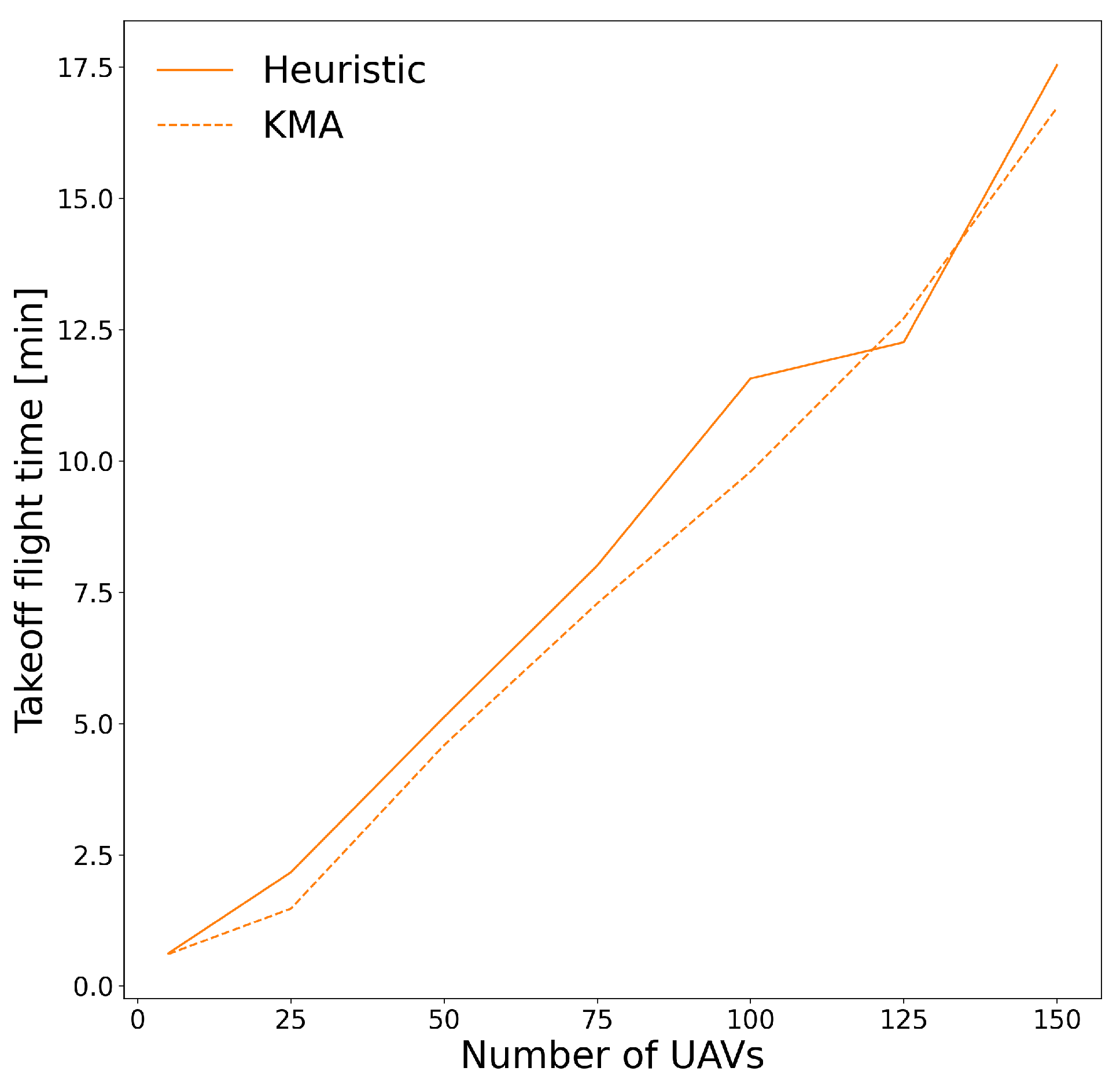
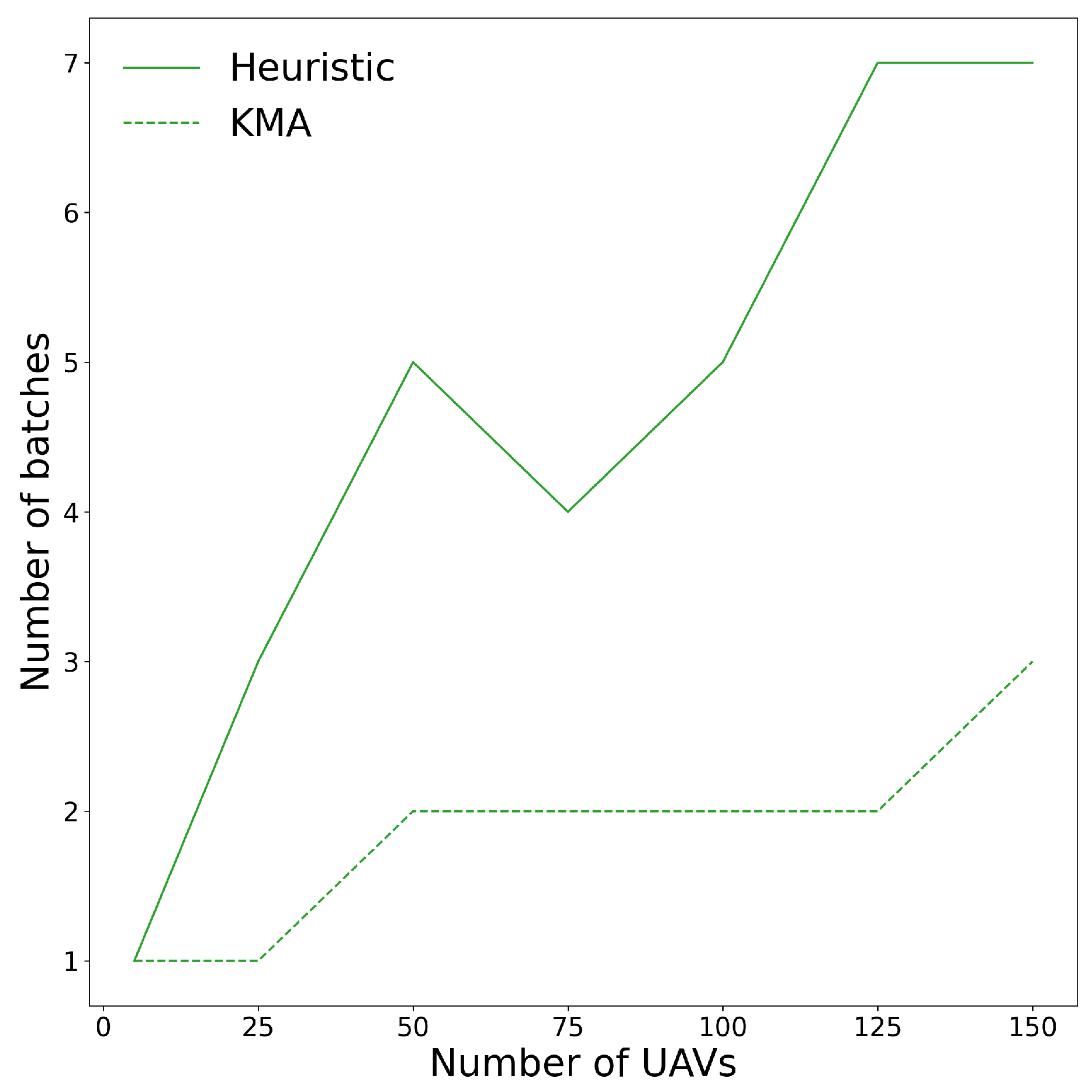
In
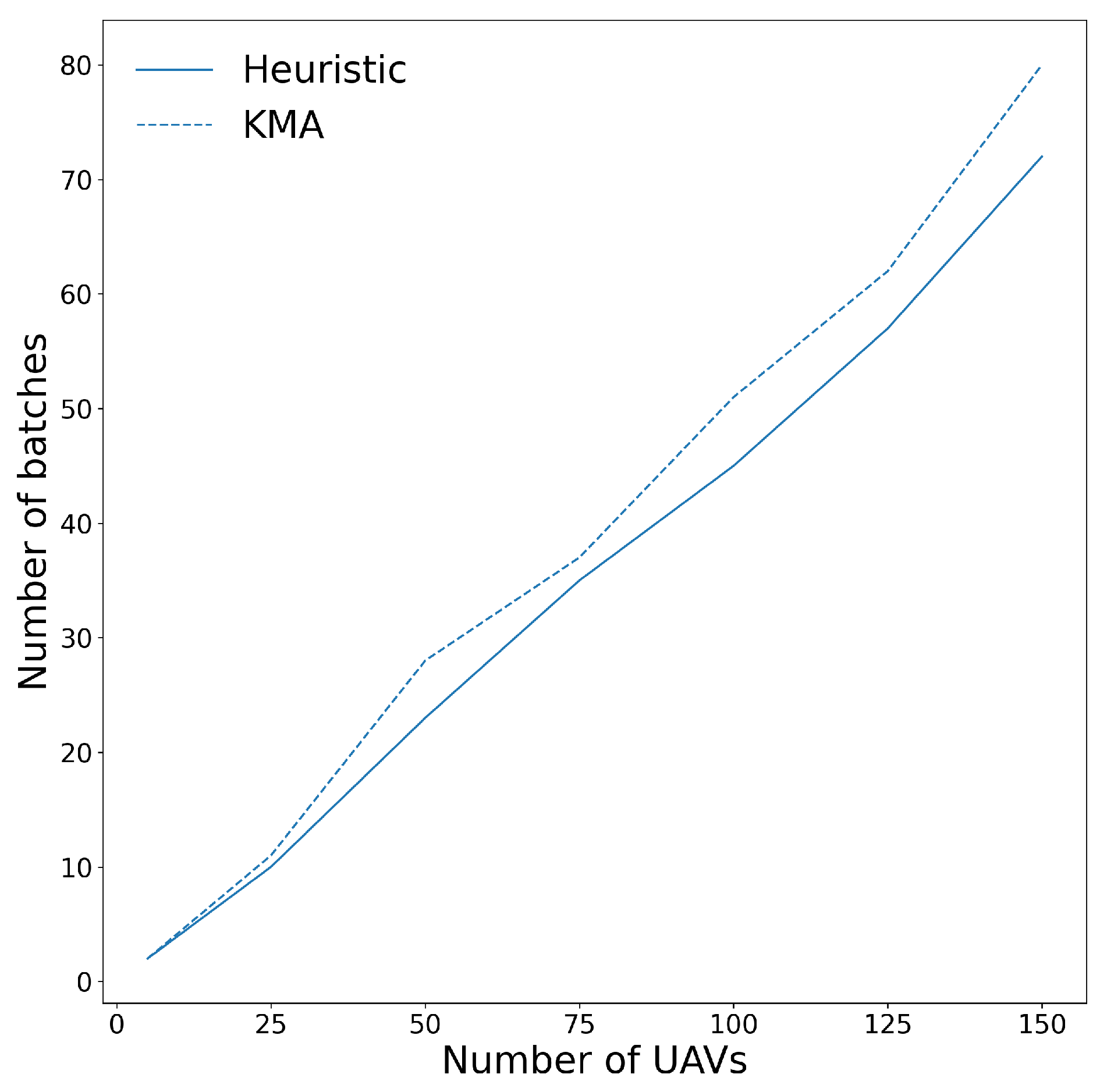
Figure 22, we visualize the take-off flight time of the two proposed assignment algorithms in the circular formation. As we can see in the figure, the heuristic provides higher times than its opponent, except for the simulation carried out with 125 UAVs. On this occasion, as we can see in
Figure 23, the heuristic that previously had a number of batches higher than KMA, now needs about 15 fewer batches. However, despite this large difference in terms of total number of batches, we only achieve an overall improvement of 0.5 min. Finally, in the test run with 150 UAVs, we see that the heuristic still continues to provide a smaller number of batches, but this time its take-off flight time is almost a minute slower than the KMA. With this last simulation, we can confirm the importance of minimizing the total displacement distance. In it, the heuristic with a smaller number of batches obtains a greater time of flight, mainly due to the fact that they must travel greater distances.
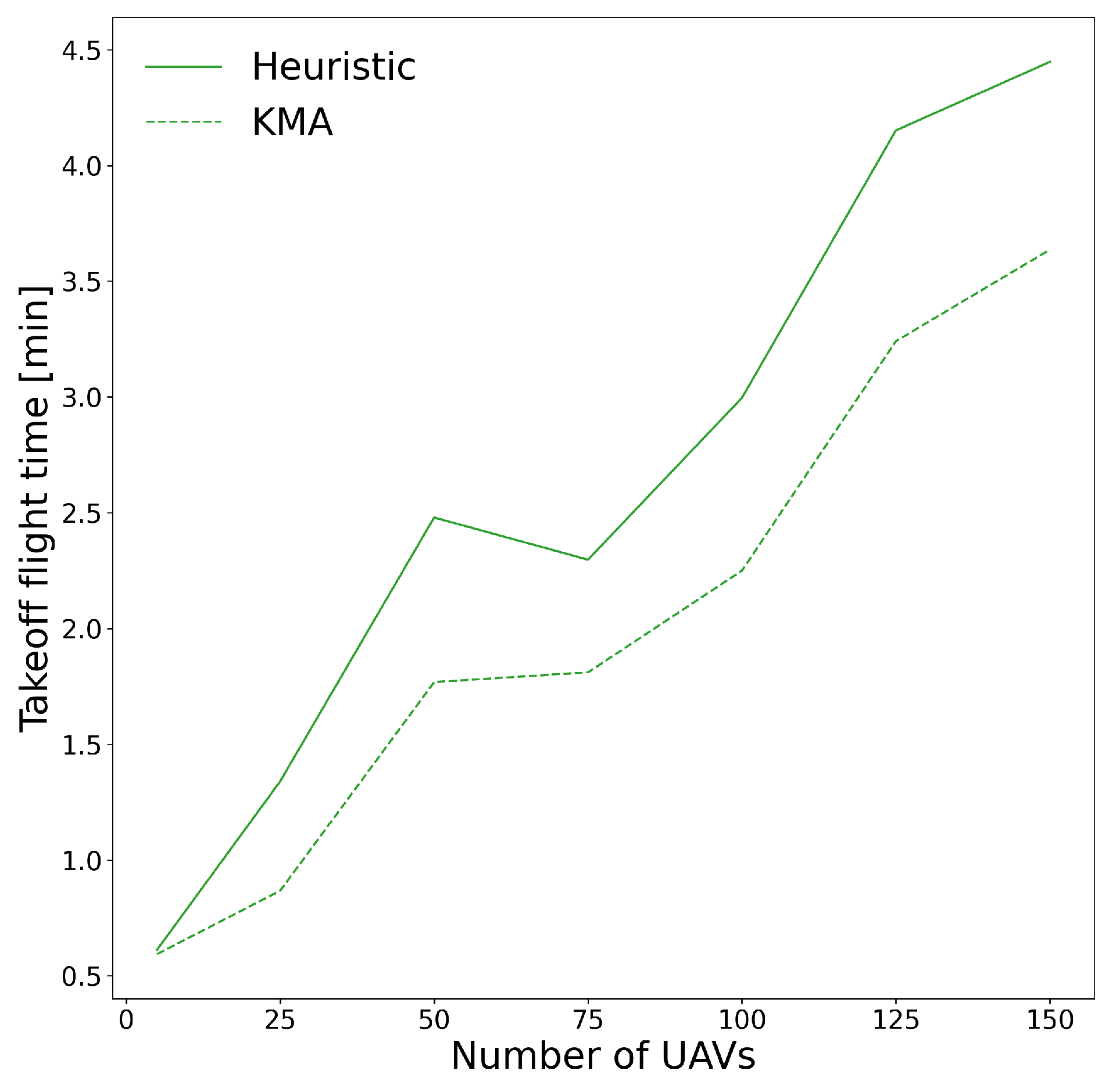
Figure 24 shows the take-off flight time of the two proposed assignment algorithms in the linear formation. Here, we observe that, except in the first experiments carried out up to 50 UAVs, the heuristic provides a more efficient solution both in take-off flight time and in the number of batches (see
Figure 25). In this case, as the total distance that the swarm has to travel to form a line in the air is very high, the difference between both algorithms is not so significant. For this reason, we observe a different effect compared to the circular formation, where with a smaller number of batches, a worse take-off time was obtained. Therefore, for the test carried out with 150 aircraft, the heuristic achieves an improvement of 1.5 min with respect to the KMA algorithm.
Finally,
Figure 26 presents the take-off flight time of the two proposed assignment algorithms in the matrix formation. We find that KMA provides better performance in all the experiments with different amounts of UAVs. The justification of the collected times is mainly due to the fact that the number of batches obtained using the KMA is quite optimal (see
Figure 27). This is due to the fact that, despite having a considerable number of UAVs, take-offs can be carried out in just two or three batches.
In conclusion, after examining the behavior of the two assignment algorithms for the three possible formations, we cannot clearly choose one option. This is because, while the KMA algorithm obtains better take-off flight time for the matrix and circular formations, it fails to obtain the best results for the linear one. However, it is important to emphasize that, with both algorithms, similar times are obtained, except for the matrix where the heuristic provides a low performance compared to KMA. Since most realistic scenarios with many UAVs are expected to use compact flight formations such as the matrix, we believe adopting our algorithms in combination with KMA for position assignment is a robust approach.
5.7. Summary of Findings
In this section, we have performed many experiments, and discussed our findings from the experiments. Now, we summarize these findings in order to intuitively display the comparative effects of the different algorithms.
In experiment 1, we searched for the ideal granularity value. This value applies to the CSTH algorithms only. In our experiments, we found that a granularity value of two meters is ideal in order to achieve the best results. A higher value will lead to missed conflicts, and a lower value will increase the computational time unnecessarily.
In experiment 2, we compared the computational time between the various CSTH algorithms. As expected, the version with both optimizations (RSR and DTD) if able to finish the computations faster than the others. The speed-up depends highly on the formation and the number of the UAVs, but it ranges from 4× to 20×.
In experiment 3, we compared the calculation time of the CSTH+RSR+DTD and ED_CSTH algorithms. We found that, for the circular and matrix formations, CSTH+RST+DTD is the fastest option. However, in the case of the linear formation, the ED+CSTH algorithm is faster. Since, on average (considering all formations) the ED_CSTH algorithm is faster, we suggest using that algorithm as default, and only switch to the other algorithm when the formation is known (and not linear).
In experiment 4, we compared the take-off time for the entire take-off process. In this case, we compared the traditional sequential method with our semi-sequential approach (using the ED_CSTH algorithm). In all cases, a huge time improvement has been made. In
Figure 21, we show the exact time improvements, for each possibility. In the best cases, when we use many UAVs (i.e., 150), a time gain between 8.8× and 16× is achieved (depending on the formation).
In our last experiment (experiment 5), we compare the influence of the different assignment algorithms (which were developed earlier in [
7,
8]). After our experiments, we could not clearly choose one option, as both methods are performing quite well. In some cases, the KMA performs better (matrix and circular formations), while in other cases the heuristic performs better. Therefore, the final decision will depend on the number of UAVs, and the formation used.
6. Conclusions
In this paper, we address the problem of achieving an efficient and yet secure take-off of UAV swarms. To this end, two collision detection approaches have been proposed: one based on spatial discretization of UAV trajectories (CSTH), and another one based on Euclidean geometry (ED_CSTH).
Their goal was to optimize the computation time necessary to detect possible conflicts on the take-off trajectories so as to ensure a safe take-off procedure. In addition, a mechanism for grouping drones into batches has also been implemented; it allows them to be grouped in a way which ensures that, during their take-off, the safety distance is guaranteed at all times.
A detailed analysis of the results using the ArduSim simulator shows that the proposed schemes are able to substantially improve take-off time (>90%) compared to the more standard sequential approach, providing the same reliability and safety as the latter.
Finally, the behavior of the proposed solutions, when combined with the KMA and Heuristics algorithms for initial position assignment, has been examined. In this case, it has not been possible to clearly choose a winning option because it depends on the specific aerial formation used, although the KMA approach seems to be the most reasonable choice considering realistic conditions.
As future work, we will study how to reduce the total number of resulting UAV batches in some of the regular formations studied to further reduce the take-off time, while still avoiding any risk of collision. To this end, we plan to also include the time factor in our risk analysis.


