Application of Weld Scar Recognition in Small-Diameter Transportation Pipeline Positioning System

Abstract

In order to improve the positioning accuracy of the pipeline inspection gauge (PIG), a pipeline positioning method, based on weld location, is proposed. The position of the welding scar is recognized by wavelet transform modulus maxima (WTMM). Equidistant welding scars provide positioning references to the strap-down inertial navigation system (SINS)/dead reckoning (DR) navigation system, which is the positioning algorithm in PIG. The following improvements have been made in relation to prior research. First, we suggest a selection strategy for the optimal mother wavelet and decomposition level; based on the strategy, WTMM can recognize the collision response between the PIG and submerged weld in the burst noise for the inertial measurement unit (IMU) output. Then, characteristic position (CP), which is the site of the weld scar, and non-holonomic constraints are utilized to decrease the position and the attitude error. By doing such, the SINS/DR/CP algorithm is proposed. The positioning error of the modified algorithm is 0.129% in the experiment, which performs better than other algorithms.

1. Introduction

Pipelines play an important role in resource transportation. The trenchless pipeline detection method protects the performance and structure of the inspected object [1]. Data and mathematical models are utilized in the detection of underground pipelines [2,3]. Many devices are also employed in trenchless detection, including ground penetrating radar [4], ultrasonic [5,6], Raman distributed fiber sensor [7], and magnetometer [8]. These sensors are affected by pipe material, buried depth, edaphic condition, and fluid type etc. [9]. To broaden the scope of its application, a detecting method based on strap-down inertial navigation system (SINS) is proposed. SINS is an autonomous navigation system that does not rely on any external information nor on the radiating energy to the outside. However, the positioning error gradually accumulates over time.

As the core components of inertial measurement unit (IMU), the gyroscope and accelerometer measure the acceleration and angular velocity of the pipeline inspection gauge (PIG) (Figure 1); therefore, the position can be calculated via SINS mechanization [10]. In a pipe detection with a small nominal diameter that is less than 50 mm [11], a small-sized micro electromechanical system IMU (MEMS-IMU) is always utilized.

The multi-sensor fusion algorithm can suppress the sensor error and the SINS cumulative error. Odometers (ODs), above ground markers (AGMs), geomagnetic information, and gravimeters provide observation information. The extended Kalman filter (EKF), adaptively adjusted cubature Kalman filter (ACKF), and other improved algorithms are applied for optimal estimation [12,13,14,15]. In small-diameter pipe detection, some researchers focus on the special structure of the pipeline since sensors precision is limited by the size of PIG. Guan utilizes non-holonomic constraints to correct PIG attitude errors [16] since the cylinder-shaped PIG maintain its azimuth and pitch angles constantlywithin each straight pipeline segment. This method only constrains attitude, and does not directly correct the relative positioning of the PIG. A method to provide reliable positioning information for PIG is necessary, especially in underground pipelines where it is difficult to obtain external positioning signals.

The pipeline junction (PJ) is used to determine the location of straight pipes, where the PIG is subject to fixed non-holonomic constraints. So, extracting pipeline junction is also an important step. Some researchers use wavelet transform to extract pipeline junction [17,18]. The selection of the specific mother wavelet and the compatibility of decomposition level are fundamental for wavelet-based processing. However, the above studies do not explain much about the wavelet selection strategy based on the collision characteristics. Moreover, we notice that, in the pipeline detection, in addition to the collision response between PIG and the weld (one type of the pipeline junction), the measurement data has rhythmic burst noise. The noises come from pulling force of manual operation. When the amplitude of collision response and rhythmic burst noise are similar, it may cause misrecognition for the weld. Up until this point, no researchers had studied the recognition of weld scar in a strong noise surrounding in pipeline detection. Ways to extract the characteristic information of the pipeline under the interference of noise is another problem.

To solve the above two problems, wavelet transform modulus maxima (WTMM) is first carried out to identify the location of the weld under the interference of noise. Then, we introduce a pipeline detection method based on SINS/dead reckoning (DR) algorithm and characteristic positions (CP) to enhance the positioning precision in small-diameter pipeline. CP is the site of collision response in the measurement data, which is the location of the weld scar. This method involves using a pair of CPs to establish the constraint vector in the straight pipe and optimizes the parameters. The content in Section 2, Section 3, Section 4 and Section 5 are mainly studied. In Section 2, we model the collision response of the weld scar, and analyze the cause of burst noise. In Section 3, we propose a strategy to choose mother wavelet and decomposition level, and accurately identify the CPs. In Section 4, we utilize the attitude and position constraints of the CPs to establish the state equation and observation equation of the navigation system. In Section 5, we undertake an experiment to evaluate the SINS/DR/CP algorithm, and provide references for parameter optimization.

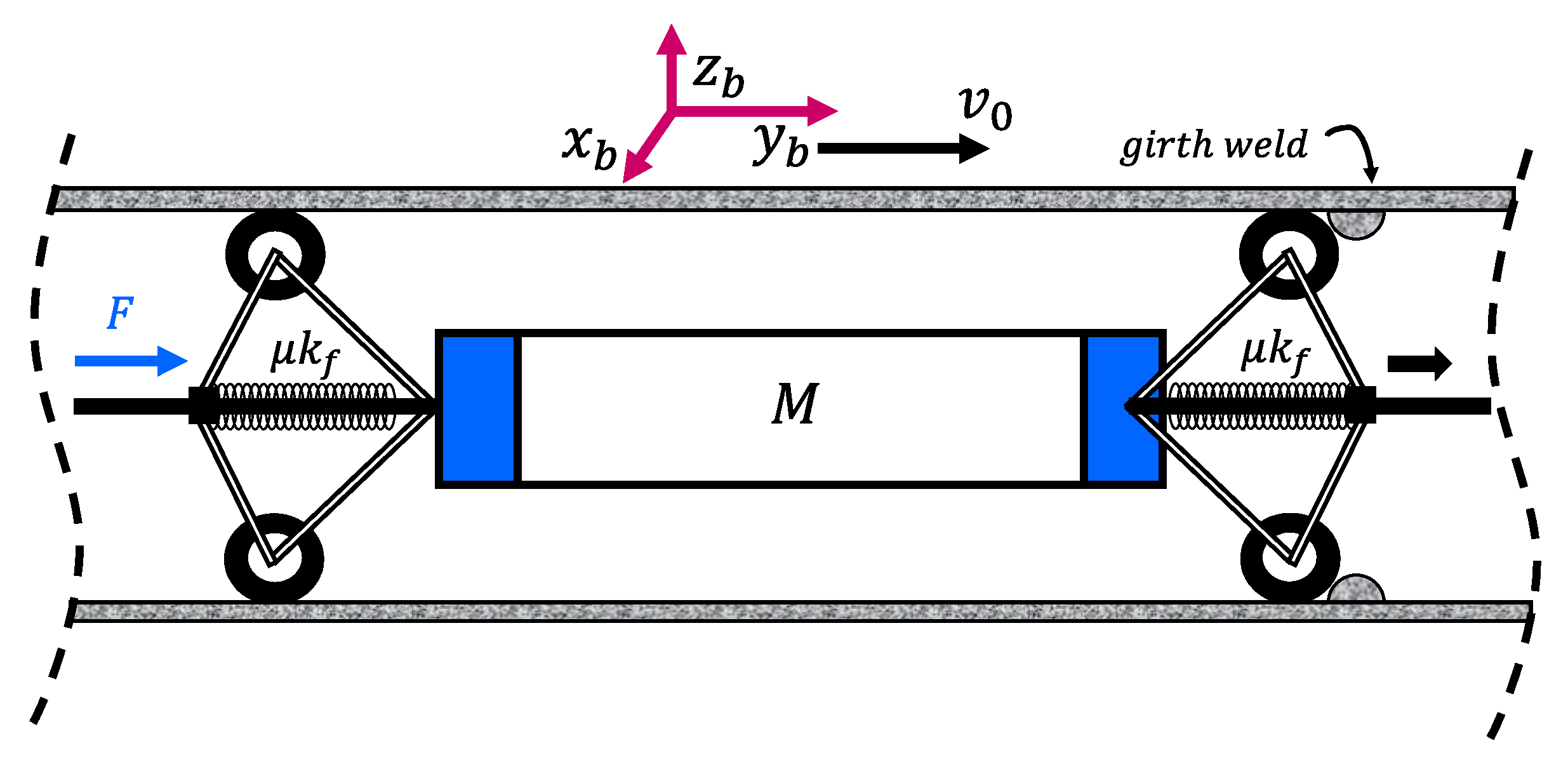
2. Collision Modeling and Noise Analysis

As one of the pipeline junction, welding technology is widely used because of its strong joints, superior airtightness, and great dependability. It is sensitive enough for IMU to capture the sudden collision between PIG and the weld. It is assumed that the PIG structure and the girth weld are isotropic along the circumference, so that only a cross section of the PIG body and pipe could be considered. The two-dimensional dynamic model is presented in Figure 2 to explain how the PIG collides with and passes through the girth weld. There are two springs in the front and rear of the PIG model. The force driving the PIG is not constant while the PIG is passing through the weld [19], the motion equation can be expressed as:

$$M\ddot{x}+\mu k_{f}a+\mu k_f(a+x)-F(v_0-\dot{x})=0$$

(1)

x is the displacement on the y axis in body coordinate system $O{x}_b{y}_b{z}_b$ (m); M is the mass of the PIG (kg); $\mu$ is the coefficient of friction between the PIG and the pipe wall; a is the interference of the system; $k_f$ is the stiffness of the springs (N/m); F is the driving force in the pipe (N); $v_0$ is the initial speed, expanding the nonlinear function $F(v_0-\dot{x})$ around the point $v=v_0$ and omitting the higher-order terms, as follows:

$$F(v_0-\dot{x})=F\left(v_0\right)-{\left.\frac{dF}{dv}\right|}_{v=v_0}\dot{x}$$

(2)

the variable of F is v, and $\dot{x}$ is used to maintain consistency with the following equations. Substituting (2) into (1), ${\left.\frac{dF}{dv}\right|}_{v=v_0}=k_1$, in following normal form:

$$M\ddot{x}+2\mu k_{f}a+\mu k_{f}x-F\left(v_0\right)+k_1\dot{x}=0$$

(3)

where $2\mu k_{f}a$ is the stable driving force, $k_1$ is the value of the first-order derivative at the point of initial speed, and $k_1=\frac{4\mu k_{f}a}{v_0}$, (3) can be expressed in a simple way:

$$\ddot{x}+\frac{k_1}{M}\dot{x}+\frac{\mu k_f}{M}x=0$$

(4)

the initial conditions are $t=0$, $x\left(0\right)=0$, $\dot{x}\left(0\right)=v_0$, and the solution is:

$$x\left(t\right)=\frac{v_0}{2\omega \sqrt{n^2-1}}\left[e^{(-n+\sqrt{n^2-1})\omega t}-e^{(-n-\sqrt{n^2-1})\omega t}\right]$$

(5)

where ${\omega }^2=\frac{\mu k_f}{M}$ is the inherent characteristic and $n=\frac{k_1}{2\sqrt{\mu mk}}=\frac{2a}{v_0}\sqrt{\frac{\mu k_f}{M}}$ is the damping coefficient of the system. The collision response instantaneously changes the output of the IMU, resulting in the decrease in positioning accuracy.

We analyze the collision response in the pipeline experiments, the data in Figure 3 and Figure 4 are from the experiments designed in Section 5. Figure 3d is a segment of the accelerometer measurement data in the pipeline experiment, the red dots mark the collision. As shown in (a), the change in amplitude is similar to Equation (5); (e) is the amplitude of the collision response in the frequency domain. In the high-frequency domain, the experimental data noise is fat-tailed distribution, and the simulated data noise is Gaussian white noise. In the low-frequency domain, the experimental data and simulated data have similar distributions, which can verify the rationality of Equation (5). Additionally, there are many rhythmic burst noises caused by the uneven pulling force in the experiment, as shown in Figure 3a,c. If the noise location of the IMU and odometer output are the same, it can be considered that the instantaneous movement rather than the sensor fault lead to the burst noise.

Figure 4 shows the consistency analysis of IMU and odometer. In Figure 4, (a) is the discrete velocity measured by odometer (m/s); (b) is the detail coefficient of the wavelet decomposition of (a), the burst noise of the velocity can be extracted by wavelet decomposition; (c) is the wavelet decomposition of the accelerometer measurement data, the light blues mark the spikes successively. By comparison, the noise spikes in (b,c) appear in the same location; (d) is the wavelet decomposition of the accelerometer output in another pipeline experiment, in which the frequency of applied pulling force is changed. As shown by the red marks, the location of the spikes in (d) has been significantly changed compared to (c). Therefore, rhythmic bursts noise caused by uneven manual operation.

3. Characteristic Position Recognition

Wavelet transform (WT) contains time information. The vanishing moment is usually utilized to compress matrix and define the concentration degree of wavelet energy—the higher the order, the sparser the matrix. In signal detection, high-order vanishing moments help highlight the singular part of the signal. Therefore, the singularity can be detected by wavelet transform. Mallat and Hwang propose the maximum modulus of wavelet transform to judge the singularity of the signal, and define Lipschitz index to quantify the singularity [20]. In this paper, WTMM is employed to de-noise the IMU measurement data, and the denoising results are decomposed of wavelet based on a different level, j, from which we can obtain a series of CPs. The noise reduction principle of WTMM are as follows.

If $f\left(t\right)$ meets the following conditions in $t_0$:

$$|f(t_0+h)-P_n(t_0+h)|\le A|h{|}^{\alpha },n\le \alpha \le n+1$$

(6)

where h is a small quantity, P is the Taylor expansion polynomial of degree n of f in $t_0$, $\alpha$ is the Lipschitz index, then it can characterize the singularity of $f\left(t\right)$ at $t_0$, and the singularity becomes weaker as $\alpha$ increases. If $t\in [a,b]$, then the mother wavelets are continuously differentiable, and it attenuates in the form of $O\left[\frac{1}{1+t^2}\right]$, when $f\left(t\right)$ satisfies

$${log}_2\left|W_2^{j}f\left(t\right)\right|\le {log}_{2}A+j\alpha$$

(7)

where the Lipschitz index of $f\left(t\right)$ is $\alpha$, A is constant, $|W_2^{j}f\left(t\right)|$ is the modular maxima, and j is the scale. The signal satisfies $\alpha >0$, and the noise satisfies $\alpha <0$, which means that signal and noise can be separated as j varies. With the increase of j, we choose the alternate projection method [21] to reconstruct wavelet coefficients, then take the inverse wavelet transform.

When constructing a sequence of modulus maxima, the detail coefficient is reduced to zero through a soft threshold, and the reconstructed signal can be guaranteed to be smooth. There are three widely used principles to determine the threshold $thr$ [22]. (1) Universal threshold principle, which calculates a fixed form threshold with respect to the length of the signal, i.e., $thr=\sqrt{2{log}_e\left(n\right)}$. (2) Minimax principle, which uses a threshold $thr=0.3936+0.1829{log}_e\left(n\right)/{log}_e\left(2\right)$ to produce minimax performance for the mean square error against an ideal procedure. (3) The Stein’s unbiased risk estimate (SURE), which is an adaptive threshold selection rule by minimizing the mean squared risk. It uses a threshold $\widehat{thr}=thr\widehat{\delta }$ and $\widehat{\delta }=median\left(\left|d_k^j\right|\right)/0.6745$, $d_k^j$ is the median value of the coefficients at level j. This threshold is suitable for non-white noise models that distributes unevenly across scales, and has better results when analyzing experimental data, so we chose this threshold.

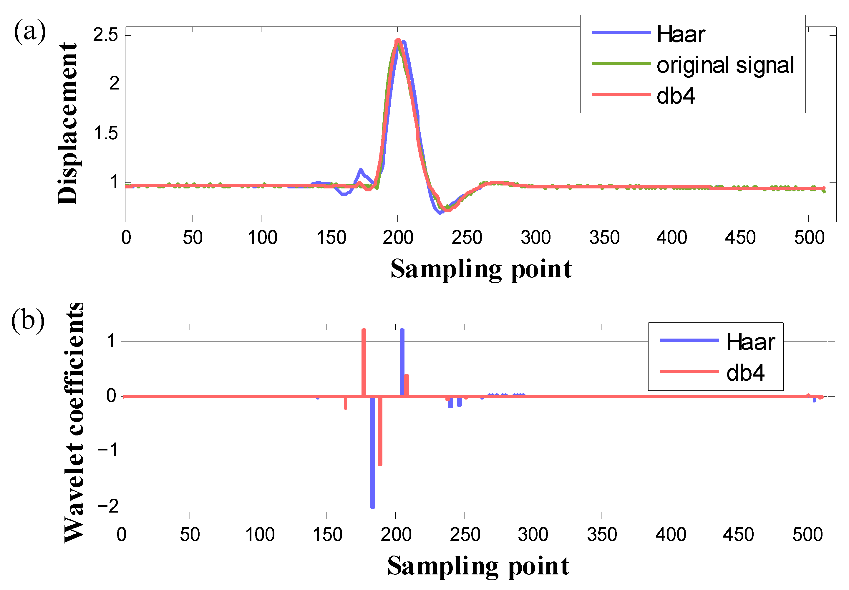
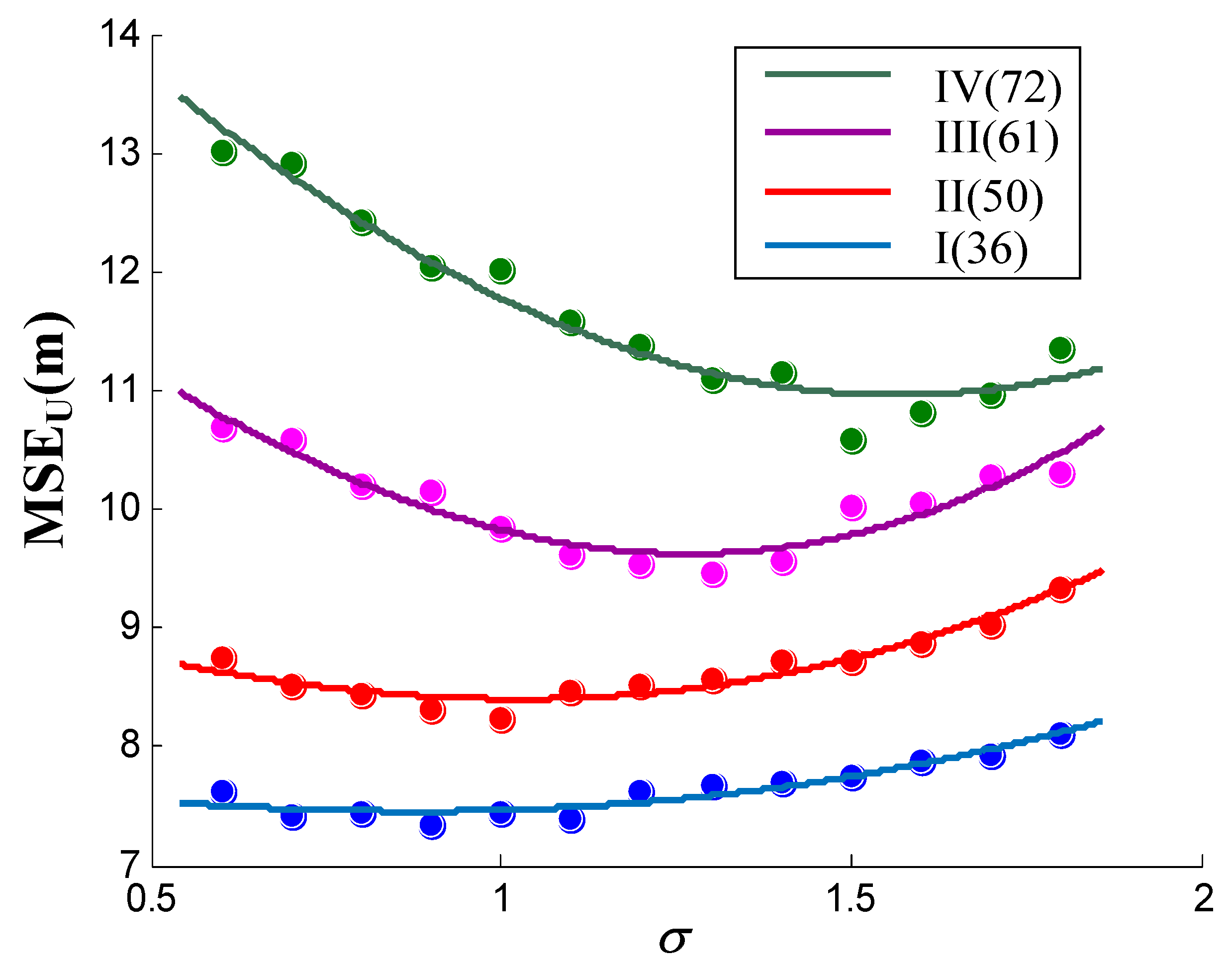
3.1. Optimal Wavelet Selection

Selection of a suitable basis mother wavelet filter is necessary for the signal processing in wavelet domain. In accordance with the definition of wavelet transform, the coefficient of wavelet decomposition will be more localized if the mother function is more similar to the analyzed signal, and this is the optimal mother wavelet. Figure 5 plots the collision signal of accelerometer measurement data in the experiment, and the wavelet coefficients (decomposition level 4) are generated and ordered. Figure 5a plots reconstructed signal of the collision response using Haar and Daubechies (order 4) filter. Figure 5b plots significant wavelet coefficients of underlying collision signal decomposed with Haar wavelet and Daubechies wavelet (db4). The plot reveals better localization property of wavelet coefficients with db4 in comparison to Haar wavelet. This signifies need of an optimal wavelet basis function for better reconstructed signal processing.

Therefore, an optimal mother wavelet selection method based on cross correlation coefficient is proposed, which is defined as

$$\gamma =\frac{\sum (X-\overline{X})(Y-\overline{Y})}{\sqrt{\sum {(X-\overline{X})}^2{(Y-\overline{Y})}^2}}$$

(8)

where X is the collision signal, Y is the mother wavelet, and $\overline{X}$ and $\overline{Y}$ are the means of the signal. Then the optimal wavelet is determined via finding the mother wavelet with the largest cross-correlation coefficient in the wavelet filter bank library.

Table 1. Comparative table of correlation coefficients with selected mother wavelet filter for CP signal under the experiment.

Wavelet Filter	$\mathit{\gamma }$	Wavelet Filter	$\mathit{\gamma }$
db1	0.2957	coif1	0.3636
db2	0.4146	coif2	0.3497
db3	0.3191	coif3	0.0506
db4	0.6391	coif4	0.0254
db5	0.2169	meyr	0.1933
db6	0.2946	sym2	0.4146
db7	0.3536	sym3	0.2941
db8	0.0172	sym4	0.6115
Haaar	0.2957	Mex Hat	0.3181

shows cross correlation coefficient of the single bit CP signal with various wavelet filters. Daubechies wavelet filter of order 4 (db4) is the optimal mother wavelet for CP extraction.

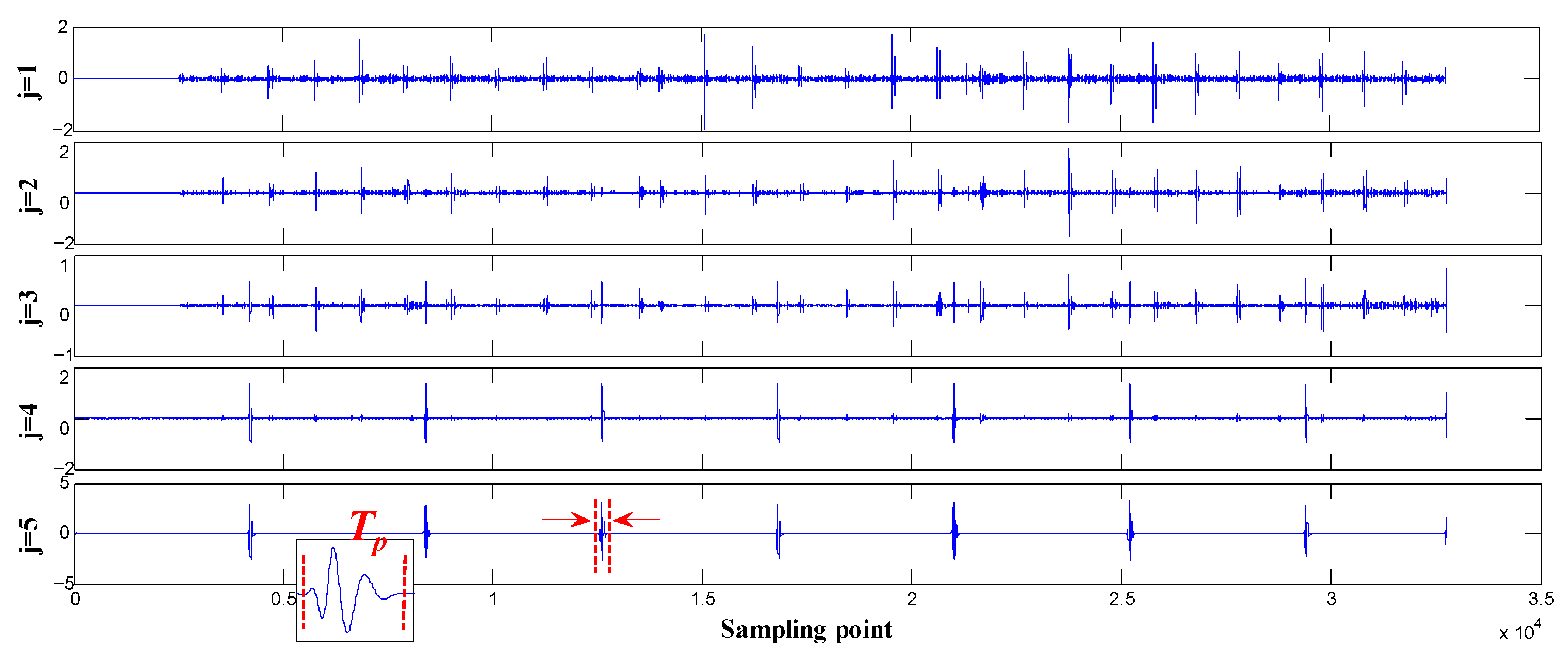
3.2. Decomposition Level Selection

Theoretically, the detail coefficient increases as the decomposition level increases. Too many decomposition level will change the trend of the signal and overreact. Too few decomposition level will not effectively separate the approximate coefficient and the detail coefficient [23]. The maximum level $maxlev$ depends on the two main operations in the procedure of wavelet decomposition: convolving with filter and downsampling, which is determined as:

$$maxlev=fix\left({log}_2(ls/(lw-1))\right)$$

(9)

where $lw$ and $ls$ are the length of filter and original signal, respectively, and fix is the round operator towards zero. For example, we utilize db4, whose corresponding filter has 8 numbers to de-noise the 6000 points of the signal. The maximum level of decomposition is 9 in this case. Usually, in order to apply different analysis requirements and reduce the decomposition and reconstruction time, the decomposition level is selected through trial and error under certain constraints. For the sake of balancing frequency resolution and computation time, decomposition level 5 is enough for pipeline surveying system.

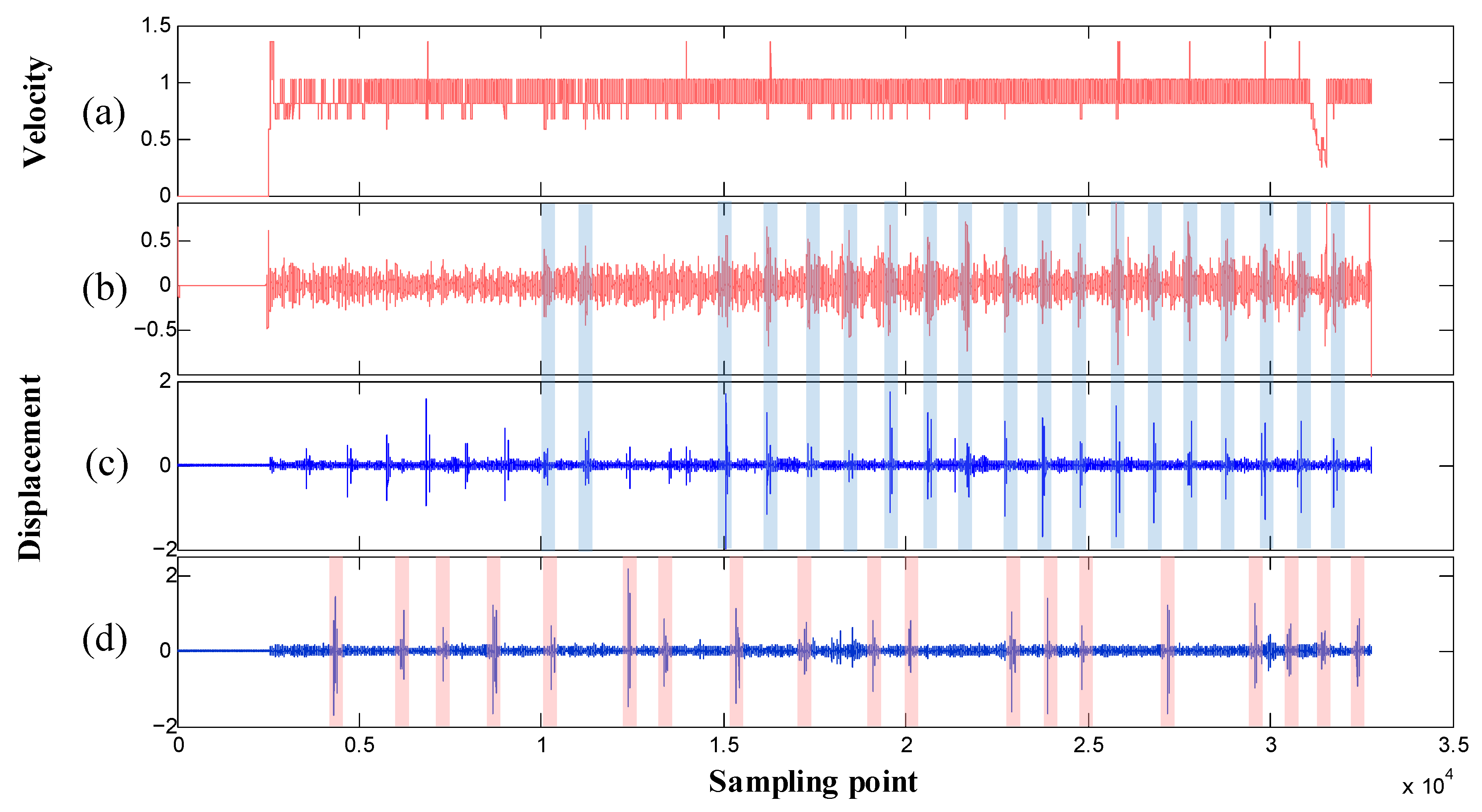
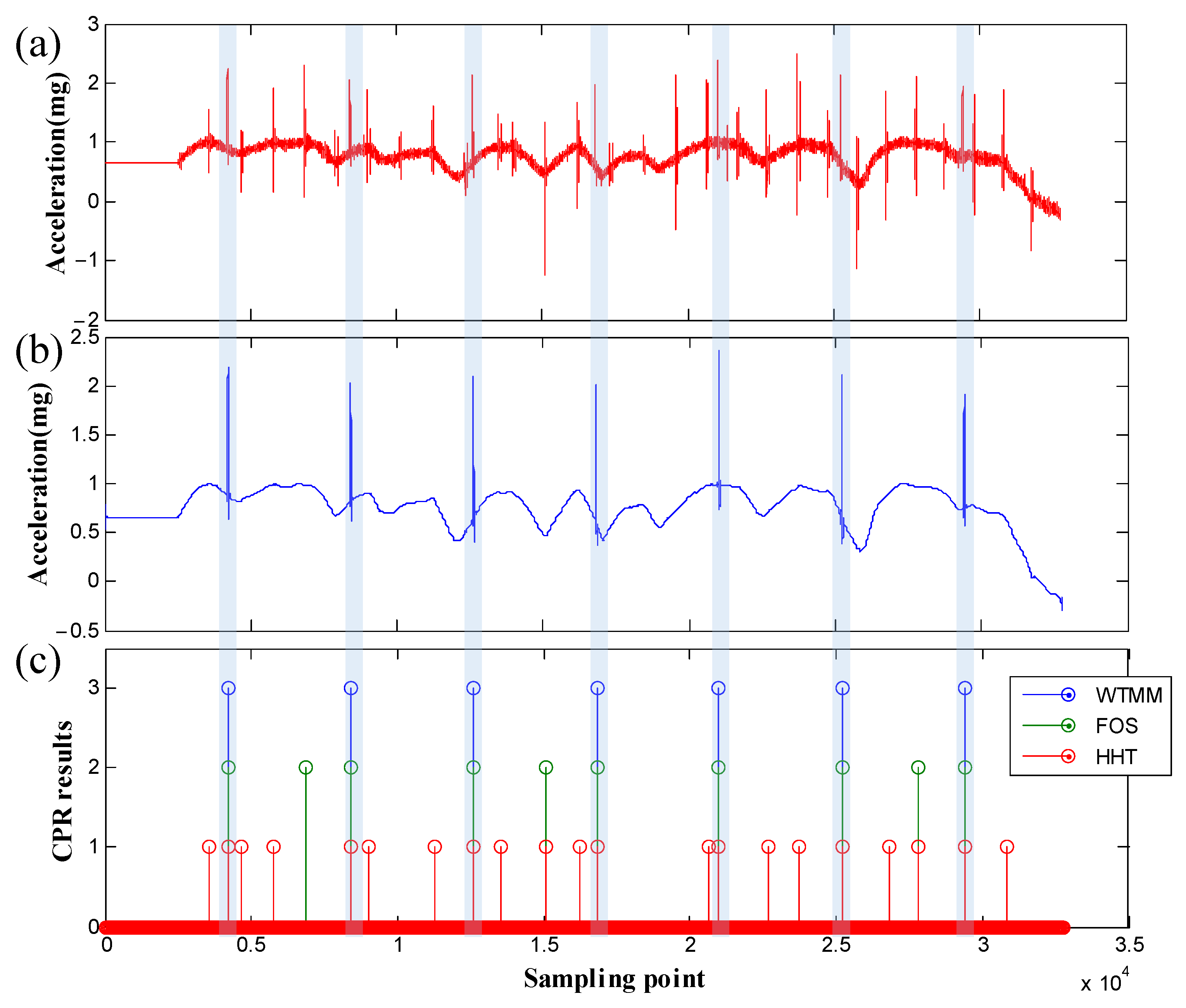
3.3. Characteristic Position Recognition

In general, gyroscope and accelerometer measurement data display stationary and singularity characteristics. However, accelerometers tend to be superior in terms of stability and accuracy of measurements, such as in the fields of bridge monitoring, pipeline deformation measurement, and structural health monitoring [24,25].

Accelerometer measurement data is decomposed with decomposition level 5. Figure 6 shows the process to extract CPs, the amplitudes of the detail coefficient denote the correlation of the moving mother wavelet and the signal, scale j is looking for the well-matched frequency. The bigger the j, the more obvious the singularity of the collision response. When j = 5, the amplitude spikes are the location of the weld, which can be regarded as the CPs, $T_p$ is collision time, CPn is a series of CPs. When j = 1, the frequency of burst noise is best match, and the position of the pulling force can be extracted. The figure reveals the local instability of the signal, which is conducive to the recognition of characteristic positions.

In addition to wavelet transform, fast orthogonal search (FOS) is a stochastic method used for time series analysis, short term signal processing, and complex system identification. After the data de-noising by FOS, the amplitude is calculated on each scale to correspond to the singularity of the original accelerometer data [16,26]. Transient analyses offer a plausible route towards leak detection due to their robustness and simplicity. The Hilbert–Huang transform (HHT) provides a modal decomposition method based on the distribution of signal extreme points, without the need to select basis functions to identify instantaneous signals [27,28]. FOS and HHT can extract signal features as well, but their identification performance in a strong noisy environment of pipeline detection has not been fully studied. As analyzed in Section 2, if the collision signal is submerged in rhythmic bursts noise, then CP may be misidentified.

In Figure 7, (a) plots the raw value of the accelerometer, (b) is the denoising data and CP recognition result of WTMM, and (c) shows the CP recognition results of HHT, FOS, and WTMM. WTMM not only correctly recognize the positions of all CPs, but also de-noises the data (choose db4 wavelet, the decomposition level is 5). FOS misidentified 3 CPs and HHT misidentified 14 CPs in 35 singular points. The recognition accuracy can be defined as $\eta =(S-S_E)/S$, S is the number of singular points, $S_E$ are the number of misidentified CPs, ${\eta }_{WTMM}=100.00\%$, ${\eta }_{FOS}=91.43\%$, ${\eta }_{HHT}=60.00\%$. That is, WTMM is more suitable for CP recognition in pipeline surveying system.

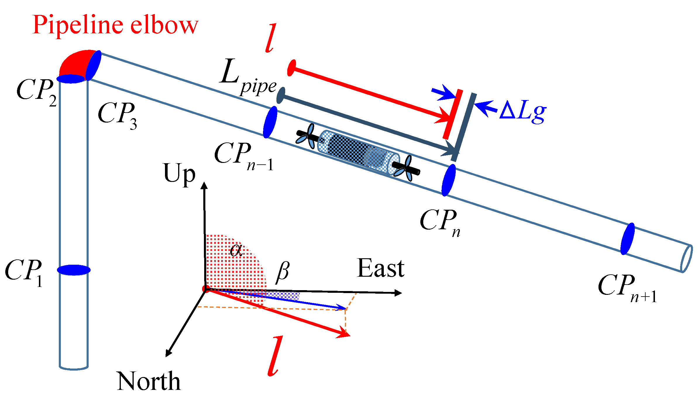
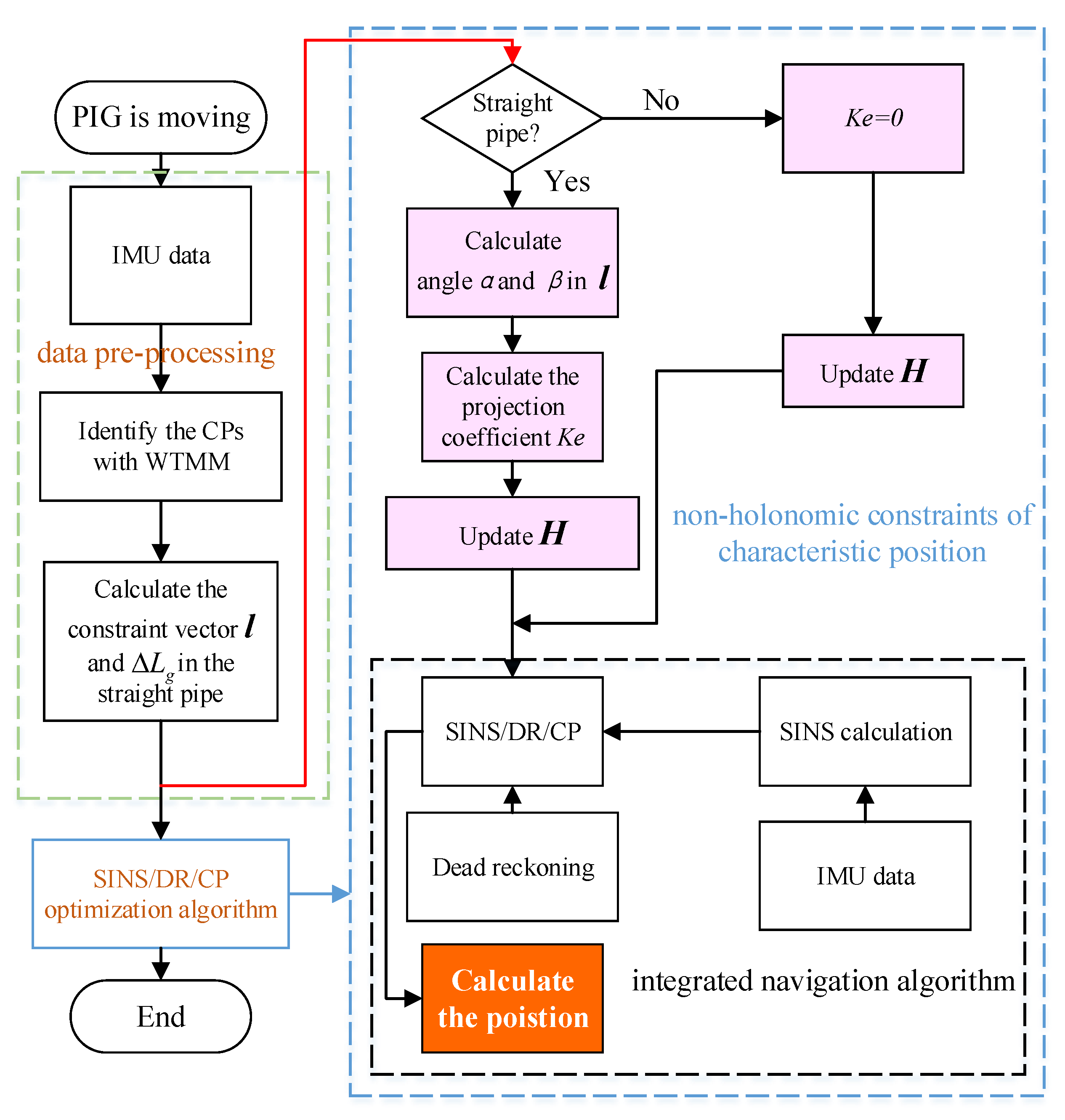
4. Models of SINS/DR/CP System

Multi-sensor data fusion is based on the error model of the sensors. The Kalman filter (KF) is always utilized for optimal estimation [29].

4.1. System Error Model

Ignoring the calibration error, the error equation of SINS/DR/CP is the following:

$$\begin{array}{c}{\dot{\varphi }}^n={\mathbf{M}}_{aa}{\varphi }^n+{\mathbf{M}}_{av}\delta v^n+{\mathbf{M}}_{ap}\delta \mathrm{p}-C_b^n{\epsilon }^b\hfill \\ \delta {\dot{v}}^n={\mathbf{M}}_{va}\varphi +{\mathbf{M}}_{vv}\delta v^n+{\mathbf{M}}_{vp}\delta \mathrm{p}+C_b^n{\nabla }^b\hfill \\ \delta \dot{\mathrm{p}}={\mathbf{M}}_{pv}\delta v^n+{\mathbf{M}}_{pp}\delta \mathrm{p}\hfill \\ \delta {\dot{\mathrm{p}}}_d={\mathbf{M}}_{pad}{\varphi }_d+{\mathbf{M}}_{ppd}\delta {\mathrm{p}}_d+{\mathbf{M}}_{pkd}\delta K_d\hfill \end{array}$$

(10)

Both the odometer and IMU are fixed on the PIG, the attitude error equation of the DR algorithm is omitted, and ${\varphi }_d^n$, ${\nu }_d$ can be replaced by ${\varphi }^n$, $\nu$ [30]; where ${\mathbf{M}}_{ij}$ are navigation coefficient matrices [31]; ${\varphi }^T$ is the attitude error vector; $\delta {\nu }^{nT}$ is the velocity error vector; $\delta {\mathrm{p}}^T$ is the position error vector; ${\epsilon }^{bT}$ is the gyroscope drift error; ${\nabla }^{bT}$ is the accelerometer zero bias error; $\delta {\mathrm{p}}_d^T$ is the odometer position error vector; and $\delta K_d^T$ is the odometer scale coefficient error. The system state vector is:

$$X={\left[{\varphi }^T\delta {\nu }^{nT}\delta {\mathrm{p}}^T{\epsilon }^{bT}{\nabla }^{bT}\delta {\mathrm{p}}_d^T\delta K_d^T\right]}^T$$

(11)

The system state equation is:

$${\dot{X}}_{21\times 1}=F_{21\times 21}{X}_{21\times 1}+G_{21\times 6}{w}_{6\times 1}$$

(12)

where

$$F=\left[\begin{array}{ccccccc}{\mathbf{M}}_{aa}& {\mathbf{M}}_{av}& {\mathbf{M}}_{ap}& -C_b^n& 0_{3\times 3}& 0_{3\times 3}& 0_{3\times 1}\\ {\mathbf{M}}_{va}& {\mathbf{M}}_{vv}& {\mathbf{M}}_{vp}& 0_{3\times 3}& C_b^n& 0_{3\times 3}& 0_{3\times 1}\\ 0_{3\times 3}& {\mathbf{M}}_{pv}& {\mathbf{M}}_{pp}& 0_{3\times 3}& 0_{3\times 3}& 0_{3\times 3}& 0_{3\times 1}\\ 0_{3\times 3}& 0_{3\times 3}& 0_{3\times 3}& 0_{3\times 3}& 0_{3\times 3}& 0_{3\times 3}& 0_{3\times 1}\\ 0_{3\times 3}& 0_{3\times 3}& 0_{3\times 3}& 0_{3\times 3}& 0_{3\times 3}& 0_{3\times 3}& 0_{3\times 1}\\ {\mathbf{M}}_{pad}& 0_{3\times 3}& 0_{3\times 3}& 0_{3\times 3}& 0_{3\times 3}& {\mathbf{M}}_{ppd}& {\mathbf{M}}_{pkd}\\ 0_{1\times 3}& 0_{1\times 3}& 0_{1\times 3}& 0_{1\times 3}& 0_{1\times 3}& 0_{1\times 3}& 0_{1\times 3}\end{array}\right]$$

(13)

is the dynamic coefficient matrix, G is the process noise distribution matrix, w is the vector of input process noise, and $C_b^n$ is the transformation matrix.

4.2. System Design Model

In SINS/DR integrated navigation algorithm, the observation vector is the difference between positions calculated by SINS and DR. In SINS/DR/CP algorithm, the pipe length is calculated by adjacent CPs, which can determine two points in the 3D space of the pipeline. The constraint vector $\overrightarrow{l}$ formed by the two points has two functions: (1) $\overrightarrow{l}$ is in the same direction as pipeline, the pitch and the azimuth angle of PIG can be non-holonomic constrained. (2) The distance of the two points $\left|\overrightarrow{l}\right|$ is the calculated length of the pipe. The difference between the calculated and the actual pipe length indicates the divergence direction and the magnitude of the positioning error. Overall, the constraint vector $\overrightarrow{l}$ can partly compensate for the systematic error.

Figure 8 plots the structure of the pipeline. $\Delta Lg=\left|\overrightarrow{l}\right|-L_{pipe}$ is the error of calculated pipe length and actual length. Constraint vector $\overrightarrow{l}$ reduces the dimensionality of configuration space and suppress the divergence of the position error. $\alpha$ is the angle between $\overrightarrow{l}$ and the vertical ($0<\alpha <\pi$); $\beta$ is the angle between the horizontal projection of $\overrightarrow{l}$ and the east ($0<\beta <\pi$). The theoretical pitch angle and azimuth angle can be determined by $\alpha$ and $\beta$. Moreover, PIG’s attitude has a significant change in pipe elbow, at this time $\Delta Lg$ is no longer applicable in the algorithm.

There are two kinds of system design models when PIG runs in different stages of the inspected pipeline. Firstly, when PIG runs in the straight pipeline segment, the system design model of SINS/DR/CP is given by:

$$\left[\begin{array}{c}\begin{array}{c}\begin{array}{c}\delta p_{CP}-\delta p_{SINS}\\ \delta a_{CP}-\delta a_{SINS}\end{array}\\ \delta {\phi }_{DR}-\delta {\phi }_{SINS}\end{array}\\ \delta {\lambda }_{DR}-\delta {\lambda }_{SINS}\\ \delta h_{DR}-\delta h_{SINS}\\ \left|\overrightarrow{l}\right|-L_{pipe}\end{array}\right]=H_{1}X-\left[\begin{array}{c}\begin{array}{c}\delta {\eta }_p\\ \delta {\eta }_a\\ \delta {\eta }_{\phi }\end{array}\\ \delta {\eta }_{\lambda }\\ \delta {\eta }_h\\ \delta {\eta }_L\end{array}\right]$$

(14)

where $\delta p$ and $\delta a$ denote the pitch and azimuth angles that calculated by SINS at the beginning of each straight pipeline segment. $\delta \phi$, $\delta \lambda$, and $\delta h$ are the longitude, latitude, and height, respectively. $\left|\overrightarrow{l}\right|$ and $L_{pipe}$ are the calculated and actual length of the pipe, respectively. $\delta \eta$ is the corresponding measurement noise.

$\delta P={\left[\begin{array}{ccc}\delta \phi & \delta \lambda & \delta h\end{array}\right]}^T$ and $\Delta Lg=\left|\overrightarrow{l}\right|-L_{pipe}$ satisfies:

$$\Delta Lg={∥\delta P_G∥}_2$$

(15)

where $\delta P_G={\left[\begin{array}{ccc}\delta P_E& \delta P_N& \delta P_U\end{array}\right]}^T$ is the projection of $\delta P={\left[\begin{array}{ccc}\delta \phi & \delta \lambda & \delta h\end{array}\right]}^T$ in navigational coordinate system $O{x}_n{y}_n{z}_n$, it satisfies:

$$\left[\begin{array}{c}\delta P_E\\ \delta P_N\\ \delta P_U\end{array}\right]=\left[\begin{array}{c}glv.\mathrm{Re}·cos\lambda ·\delta \phi \\ glv.\mathrm{Re}·\delta \lambda \\ \delta h\end{array}\right]=e\left[\begin{array}{c}\delta \phi \\ \delta \lambda \\ \delta h\end{array}\right]$$

(16)

meanwhile, under the constraints of straight pipelines,

$$\Delta Lg=K_i·\delta P_G\left(i\right)=K{e}_i·\delta P\left(i\right)$$

(17)

where $K{e}_i=\left[\begin{array}{ccc}K{e}_E& K{e}_N& K{e}_U\end{array}\right]=e\times K_i$ is the projection coefficient, where

$$K_i={\left[\begin{array}{ccc}cos\alpha ·cos\beta & sin\beta & sin\alpha ·cos\beta \end{array}\right]}^T$$

(18)

$\alpha$ is the angle between $\overrightarrow{l}$ and the vertical ($0<\alpha <\pi$), $\beta$ is the angle between the horizontal projection of $\overrightarrow{l}$ and the east ($0<\beta <\pi$); therefore, the observation matrix H is the following:

$$H_1=\left[\begin{array}{c}\begin{array}{cc}{H}_{1,2}& 0_{2\times 18}\end{array}\\ \begin{array}{ccccc}{0}_{3\times 6}& I_{3\times 3}& 0_{3\times 6}& -I_{3\times 3}& 0_{3\times 3}\end{array}\\ \begin{array}{ccccc}{0}_{1\times 6}& K{e}_E& K{e}_N& K{e}_U& 0_{1\times 12}\end{array}\end{array}\right]$$

(19)

and $H_{1,2}=\left[\begin{array}{c}\begin{array}{ccc}1& 0& 0\end{array}\\ \begin{array}{ccc}0& 0& 1\end{array}\end{array}\right]$ is the constrain matrix of pitch and azimuth angles.

Besides, when PIG running in the pipeline elbow, the system design model of SINS/DR/CP is given by:

$$\left[\begin{array}{c}\begin{array}{c}\delta {\phi }_{DR}-\delta {\phi }_{SINS}\end{array}\\ \delta {\lambda }_{DR}-\delta {\lambda }_{SINS}\\ \delta h_{DR}-\delta h_{SINS}\end{array}\right]=H_{2}X-\left[\begin{array}{c}\begin{array}{c}\delta {\eta }_{\phi }\end{array}\\ \delta {\eta }_{\lambda }\\ \delta {\eta }_h\end{array}\right]$$

(20)

and the corresponding system design matrix $H_2$ is:

$$H_2=\left[\begin{array}{c}\begin{array}{ccccc}{0}_{3\times 6}& I_{3\times 3}& 0_{3\times 6}& -I_{3\times 3}& 0_{3\times 3}\end{array}\end{array}\right]$$

(21)

During the update phase of the SINS/DR/CP algorithm, dead reckoning provides continuous new position reference. Non-holonomic restrains the divergence of pitch and azimuth angle, and the calculation error of the straight pipe length compensates for the errors. Furthermore, the displacements of IMU measurement data caused by CPs significantly decrease the positioning accuracy, as analyzed in Section 2. Increasing the level of wavelet decomposition to 9 can smooth the signal and reduce the singularity, but this method will distort the measurement data when PIG keeps still. Another method is to temporarily discard the IMU measurement data within the collision time $T_p$, and utilize the data before $T_p$. After comparison, the latter method has higher positioning accuracy. Figure 9 is the flowchart of SINS/DR/CP algorithm.

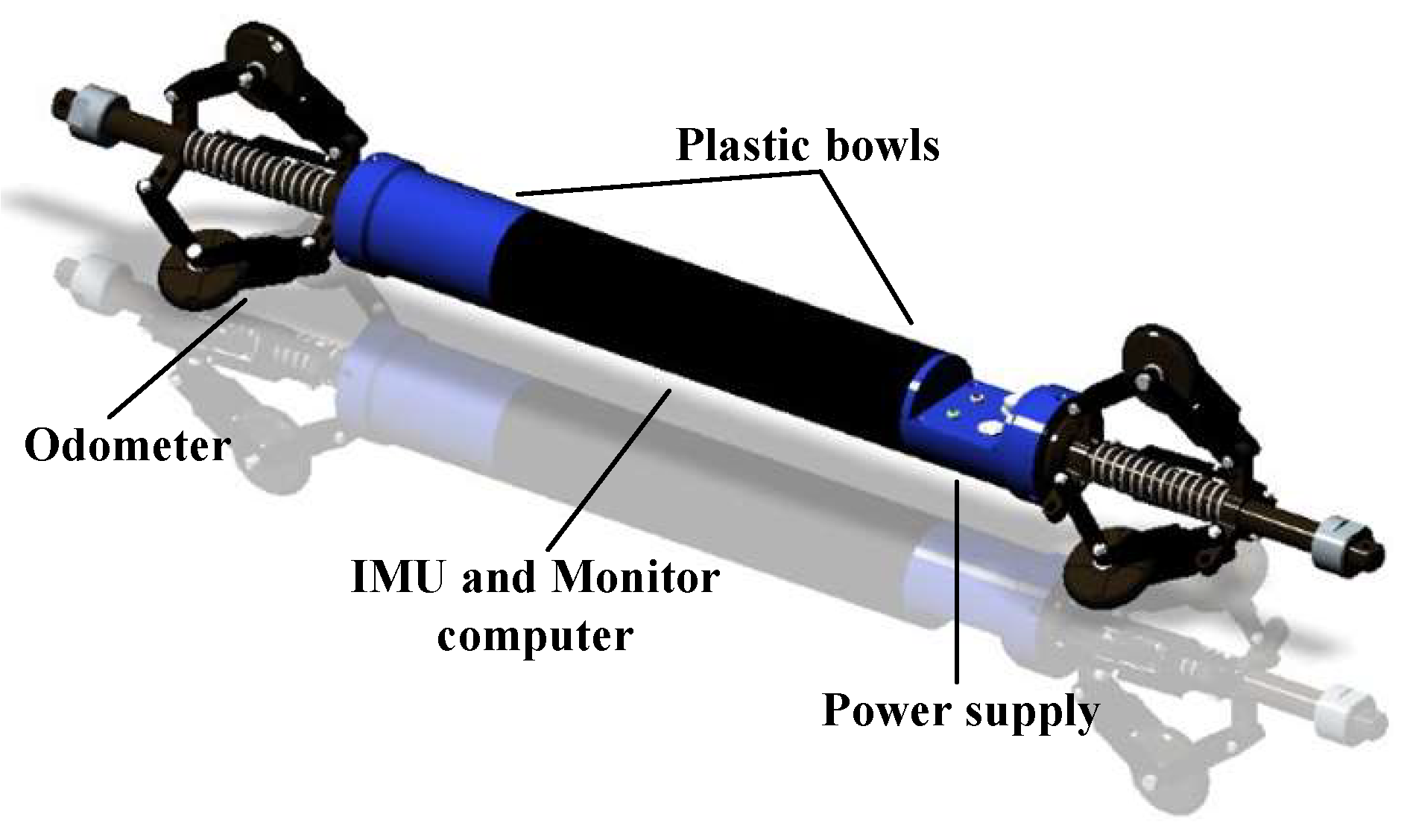
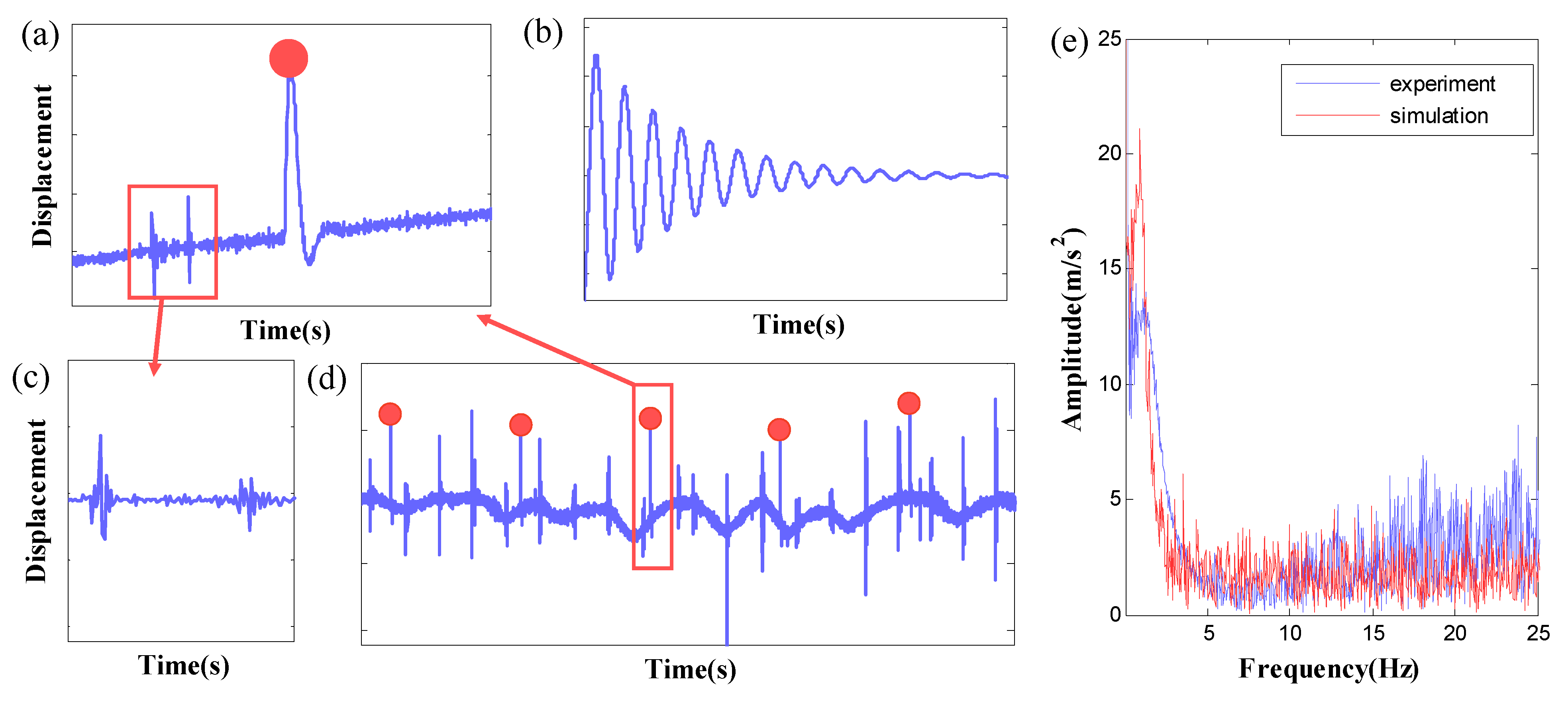
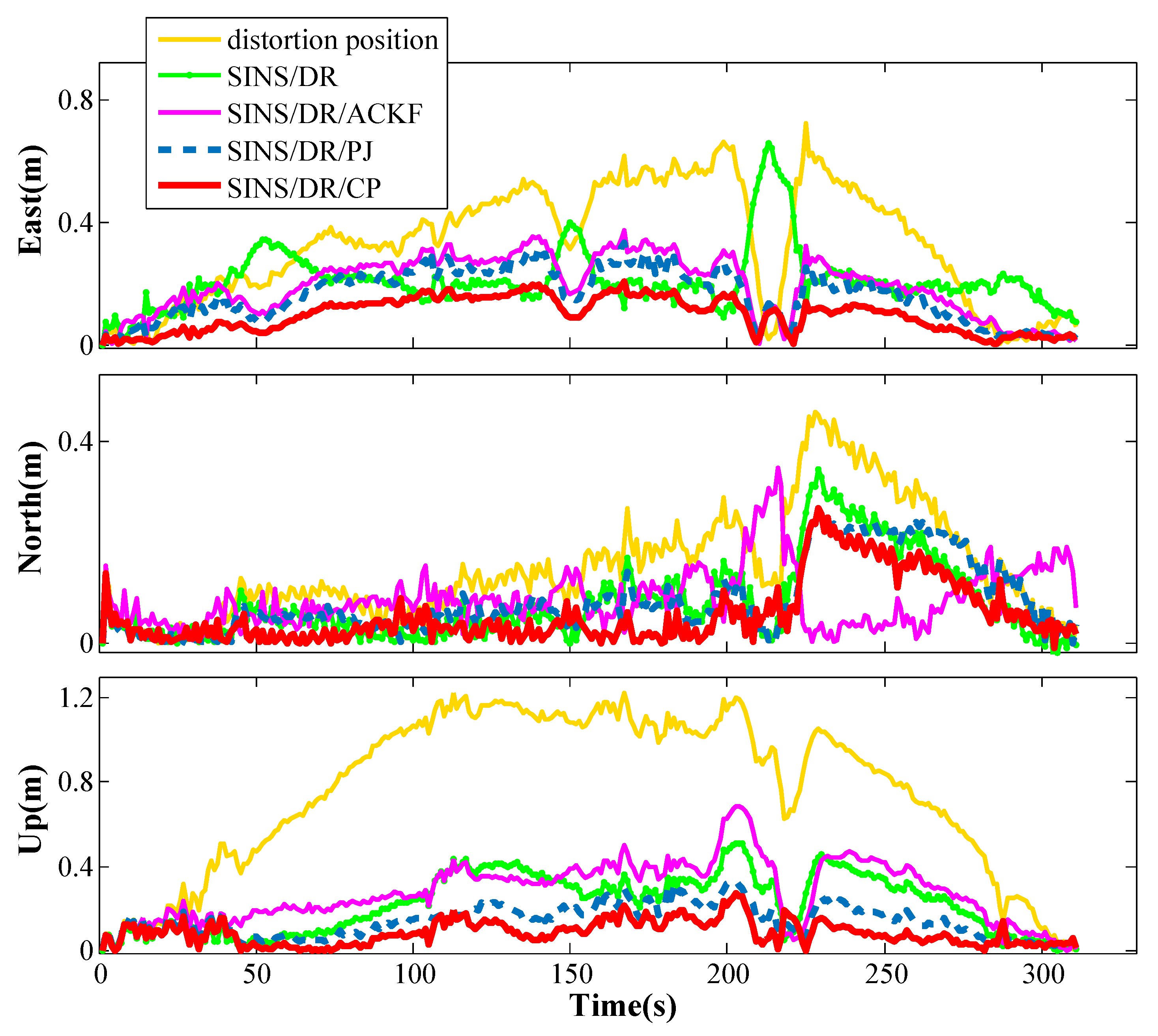
5. Simulation and Experiment

In this section, we validate the proposed method via numerical simulation and pipeline experiment. The CP recognition in the experiment has been analyzed in Section 2 and Section 3, so this section focuses on positioning results of the algorithm.

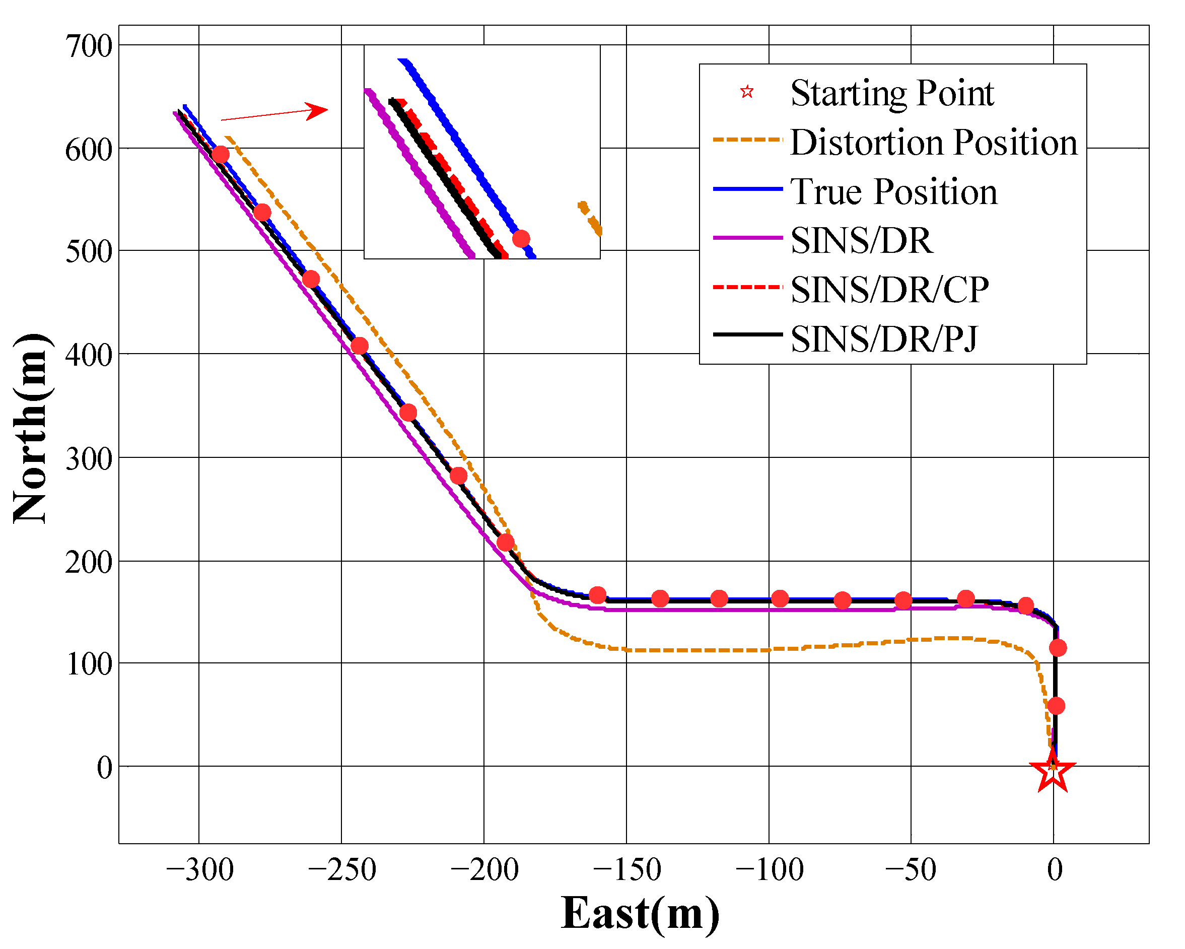
5.1. Simulation Results

In the simulated experiment, the parameters were set as follows: The experimental location was Harbin (45.7796° N, 126.6705° E), the gyro bias error was $0.5^{\circ }$/h, and the accelerometer bias error was $5\times 10^{-5}{g}_0$ ($g_0$ was the standard acceleration of gravity, $g_0$ = 9.78049 m/s²). Gyroscope and acceleration data were obtained from pipeline trajectory generator, the inertial platform misalignment angle was $\left[{15}^{\prime }{15}^{\prime }{10}^{″}\right]$, the initial velocity error and position error were both 0, the sampling frequency was 100 Hz, and the sampling time was 1000 s.

We generated the simulation pipeline trajectory, which is composed of multiple 35 m long pipes. Based on the known pipeline position, the theoretical acceleration and angular velocity values of x, y, and z axis in the inertial coordinate system were obtained. Then we added bias and random noise to the theoretical angular velocity and acceleration, and further added collision error that satisfied Equation (5). This simulated IMU measurement data in pipeline detection. After that, we recognized the CPs by WTMM. Lastly, we calculated the trajectory of the pipeline based on different methods and compared the results.

Figure 10 shows the comparison of different positioning methods. After being affected by the weld, the trajectory remains smooth, and there is no singularity caused by periodic noise. The red points are CPs, the brown line is distortion position affected by the weld, with an error of up to 40 m. The purple line is the trajectory calculated by SINS/DR. The closest trajectory is the red line, which is calculated by SINS/DR/CP algorithm. The simulation does not consider the influence of manual operation, it is necessary to design pipeline experiments to further confirm the effectiveness of the proposed algorithm.

Table 2. Positioning error of different surveying methods in simulation.

Different Methods	East (m)	North (m)	MSE(H/V) (m)
Distortion Position	15.76	48.95	(27.88; 11.41)
SINS/DR	3.73	8.58	(5.27; 2.81)
SINS/DR/PJ	3.01	6.89	(4.92; 2.68)
SINS/DR/CP	2.64	5.82	(4.49; 2.31)

summarizes the positioning error of different surveying methods in simulation.

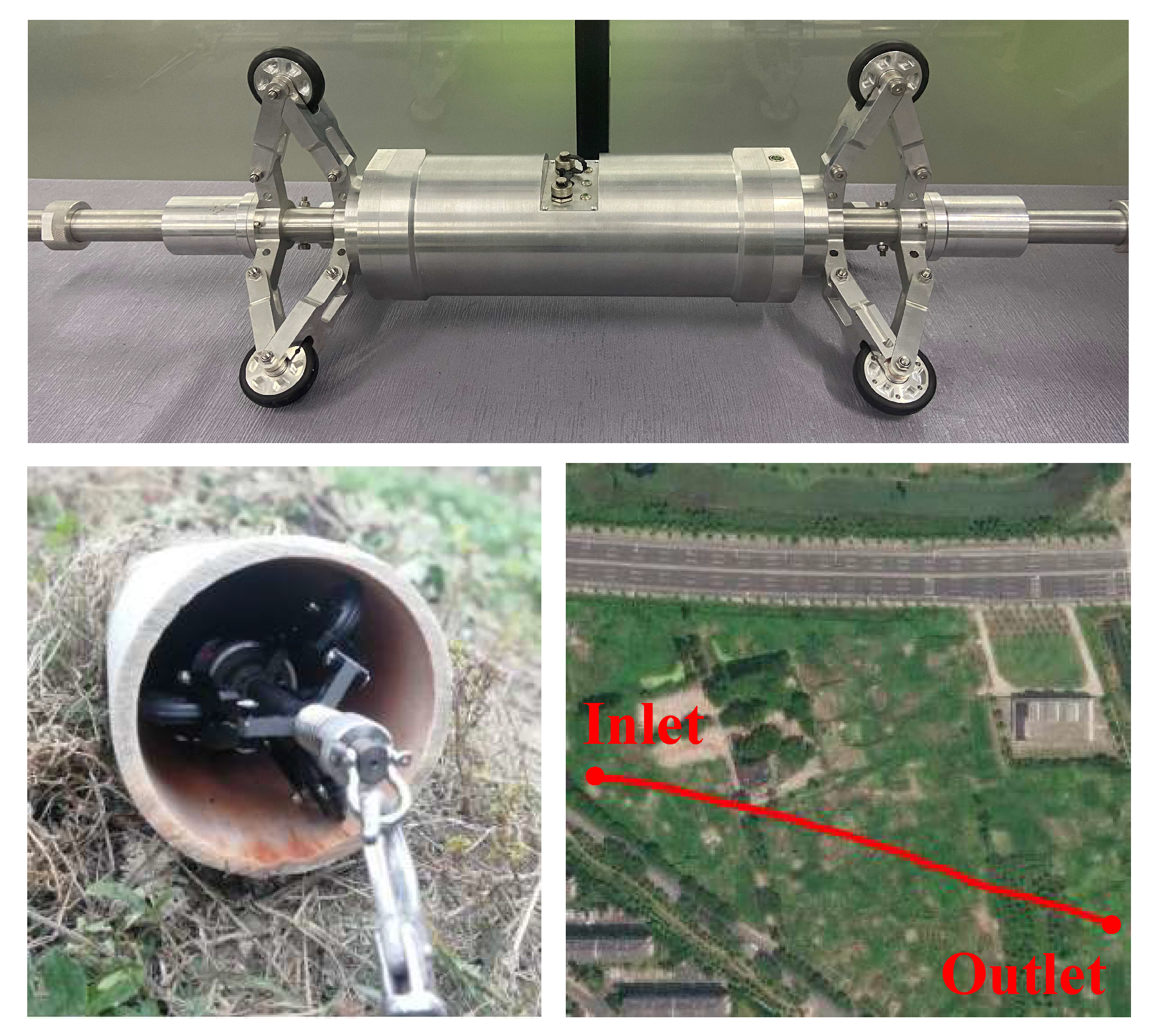
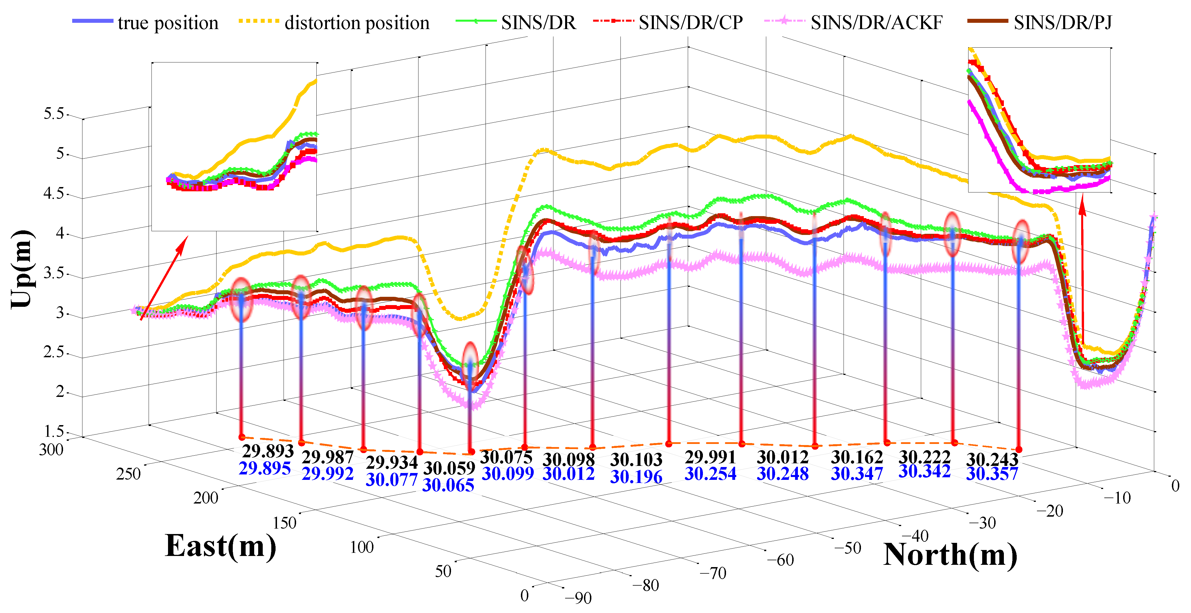
5.2. Experiment Results

A real pipeline experiment was undertaken to evaluate the proposed method. The PIG and data processing software were designed and developed in Harbin Institute of Technology. As shown in Figure 11, the experiment field was in Songjiang, Shanghai (31.1090° N, 121.1738° E). The total length of the pipeline was 300 m, which was welded by multiple 30 m long pipes. The parameters of the weld strictly followed the national pipeline welding standard ($GB$50236). The girth weld was 4 mm higher than the inner surface of the pipe, the length of the girth weld was 10 mm. The MEMS-IMU was STIM300 with an output frequency of 100 Hz. The odometer was the Hall sensor ES3114, it measured the traveled distance by counting the number of rotations of the wheels. In addition, the microprocessor was STM32 with ARM Cortex-M, the data was stored on an SD card for offline processing. The calibration results of IMU are shown in

Table 3. Calibration results of IMU.

Gyroscope	Zero Bias (°/s)	Scale Factor	Installation Error (${}^{″}$)
x-axis	0.0987	0.9875	198.231	256.325
y-axis	0.0996	1.0125	196.258	100.157
z-axis	0.1012	1.0079	299.345	100.108
Accelerometer	Zero Bias (m/s)	Scale Factor	Installation Error (${}^{″}$)
x-axis	0.0895	0.8920	200.211	298.125
y-axis	0.1010	1.0052	199.435	100.156
z-axis	0.1123	0.9784	297.568	100.025

.

The specific steps of the experiment process are as follows:

*

Use real-time kinematic technology (RTK) to obtain pipeline real position.

*

Keep the PIG still at the pipe inlet and complete the initial alignment.

*

Follow the direction of the arrow on the PIG, push the PIG slowly into the pipe until the rear is flush with the pipe entrance, let it stand for 1 min, and pull the iron chain connected with the PIG until the PIG reaches the end of the pipeline.

*

Keep PIG still for 1 min, pull the PIG back at the pipeline inlet.

*

Repeat the above process three times.

*

Read the data stored in the SD card, and calculate the trajectory of the pipeline.

Limited by the MEMS-IMU precision, the azimuth calculated by the initial alignment was not accurate. So, we assumed that the initial azimuth was northward and rotated the calculated PIG trajectory. The rotation angle was based on the relative positions of the inlet and outlet of the pipeline. Furthermore, we adopted the forward and reverse test method, which ensured that the positioning error was minimized at the inlet and outlet of the pipeline.

Figure 12 plots the pipeline trajectory calculated by different algorithm. The red line is the positioning result of the SINS/DR/CP algorithm. RTK is regarded as the pipeline true position because of the highest accuracy. The marks in the figure are the weld locations. The black text $\left|l_{CP}\right|$ indicates the distances between two adjacent CPs calculated by SINS/DR/CP, the blue text $\left|l_{PJ}\right|$ indicates the distances between two adjacent CPs calculated by SINS/DR/PJ, both are in meters. By contrast, there is no obvious monotonic change in $\left|l_{CP}\right|$, and the amplitude is closer to the true value. Comparing the result of SINS/DR/CP algorithm with the true trajectory, as shown in Figure 13, the maximum horizontal error is 42.2 cm and the maximum vertical error is 31.7 cm in the 300 m pipeline, the positioning error is 0.129%. Similarly, the positioning error of distortion position, SINS/DR, SINS/DR/ACKF, and SINS/DR/PJ are 0.571%, 0.276%, 0.268%, and 0.178%, respectively.

SINS/DR is simple and suitable for pipeline detection system, but it accumulates errors faster. ACKF utilizes a set of cubature points to approximate the state mean and covariance of a nonlinear system with additional Gaussian noise. It is suitable for high-dimensional nonlinear problems and has good stability. However, the nonlinearity of the pipeline surveying system is not obvious, and raw gyroscope measurement data are not Gaussian distribution, so the positioning accuracy of ACKF is lower than SINS/DR/PJ. SINS/DR/PJ utilizes the non-holonomic constraints of the pipeline, and it regards the azimuth angle and pitch angle of the straight pipeline as the true value to correct the attitude. However, the length of equidistant weld is not utilized, which is exactly the pro of SINS/DR/CP. Moreover, the pipeline in the experiment is basically straight, with only small height changes. Almost the entire pipeline matches the conditions of SINS/DR/CP algorithm. The comparison results of SINS/DR/CP algorithm and other algorithms are summarized in

Table 4. Positional accuracy comparison of different surveying methods.

Different Methods	Horizontal Error (m)	Vertical Error (m)	Positioning Error	MSE(East; North; Up) (m)
Distortion Position	0.762	1.182	0.571%	(45.1; 10.51; 144.5)
SINS/DR	0.651	0.511	0.276%	(16.6; 6.5; 21.3)
SINS/DR/ACKF	0.492	0.680	0.268%	(20.1; 8.2; 30.3)
SINS/DR/PJ	0.421	0.338	0.178%	(12.3; 6.4; 12.9)
SINS/DR/CP	0.306	0.243	0.129%	(7.8; 5.6; 7.0)

, it reveals that SINS/DR/CP has the desirable positioning accuracy.

Furthermore, we notice that the frequency of manual pulling force will affect the reliability of the calculated pipe length. PIG moves instantaneously when it is pulled, which result in accumulation of displacement errors. SINS/DR/CP utilizes the calculation error $\left|\overrightarrow{l}\right|-L_{pipe}$ of the pipe length as the observation vector, which will be affected by the cumulative displacement of the PIG. Therefore, projection coefficient $K{e}_i$ in Equation (17) needs to be adjusted adaptively to weaken the influence of pulling force:

$$\widehat{K}{e}_i=\sigma \times K{e}_i=\sigma \times \left[\begin{array}{ccc}K{e}_E& K{e}_N& K{e}_U\end{array}\right]$$

(22)

where $\sigma$ is the adjustment coefficient. Four pipeline experiments are conducted with different pulling frequency in the same site. Pulling force is difficult to quantify and control, so we count the total number of accelerometer burst noise by wavelet transform, as analyzed in Figure 4. The total number of burst noise in experiment I, II, III, and IV are 36, 50, 61, and 72, respectively. After that, we adjust $\sigma$ to ask for the lowest mean square error (MSE) of the upward positioning error that changes significantly.

Figure 14 shows the impact of $\sigma$ on positioning accuracy. Obviously, frequent pulling will reduce the positioning accuracy. The green line is the data of Experiment IV, it has 72 times burst noise and has the largest mean square error compared with others. The blue line is the data of Experiment I, it has 36 times burst noise and has the highest positioning accuracy. Furthermore, the optimal value of $\sigma$ increases with the increase in the number of burst noises. When the frequency of the pulling is relatively high, $\sigma$ should take around 1.5, and when the frequency of the pulling is low, $\sigma$ should take around 1.0. In long pipeline detection, to ensure work efficiency, the velocity of PIG is usually greater than 1 m/s, which limits the method of removing burst noise by pulling the PIG smoothly and slowly. By calculating the number of burst noise in the accelerometer, positioning precision can be improved.

6. Conclusions

Miniaturization limits the choice of sensors in pipeline detection. The collision of PIG and the weld reduce the pipe positioning accuracy in pipeline detection. Odometer, non-holonomic constraints, and equidistant weld scars are crucial external updates for SINS to achieve the desirable positioning accuracy. At a pipeline detection site, it is common to manually pull the PIG, which will induce burst noise to measurement data. When the collision response between the PIG and the weld scar is submerged in the burst noise, it may lead misrecognition of the weld. This paper models the collision response as CP, proposing a CP recognition method and the improved navigation algorithm based on the equidistant CPs.

The results from the simulations and real experiment are presented to validate the proposed method and the relevant algorithm. WTMM of selecting the mother wavelet based on the cross-correlation coefficient can recognize the position of CP when it is affected by burst noise. The larger the scale, the more obvious the CP in the detail coefficient. Compared with other methods, SINS/DR/CP enables a PIG to self-orient, utilizing the equal spacing characteristics. The experimental results show that the calculated pipe length of improved algorithm is closer to the true value, and can better restrain the divergence of the horizontal and vertical error to 0.306 m and 0.243 m, respectively. The comprehensive positioning error is 0.129%. Simulation and actual test result show that the method is simple and robust, and can be used by pipeline PIG manufacturers.

The azimuth of a moving PIG remains constant for a long time in long pipelines. The azimuth estimates will gradually diverge due to low observability, then the positioning precision will decrease. In follow-up studies, researchers can focus on the observability of the azimuth and the positioning precision of PIG in pipes of different lengths.

References

1. Souas, F.; Safri, A.; Benmounah, A. A review on the rheology of heavy crude oil for pipeline transportation. Pet. Res. 2021, 6, 116–136. [Google Scholar] [CrossRef]
2. Pérez-Pérez, E.; López-Estrada, F.; Valencia-Palomo, G.; Torres, L.; Mina-Antonio, J.D. Leak diagnosis in pipelines using a combined artificial neural network approach. Control Eng. Pract. 2021, 107, 104677. [Google Scholar] [CrossRef]
3. Xiao, R.; Hu, Q.; Li, J. A model-based health indicator for leak detection in gas pipeline systems. Measurement 2020, 171, 108843. [Google Scholar] [CrossRef]
4. Lameri, S.; Lombardi, F.; Bestagini, P.; Lualdi, M.; Tubaro, S. Landmine detection from GPR data using convolutional neural networks. In Proceedings of the 2017 25th European Signal Processing Conference (EUSIPCO), Kos Island, Greece, 28 August–2 September 2017. [Google Scholar]
5. Lang, X.; Li, P.; Guo, Y.; Cao, J.; Lu, S. A Multiple Leaks’ Localization Method in a Pipeline Based on Change in the Sound Velocity. IEEE Trans. Instrum. Meas. 2019, 69, 5010–5017. [Google Scholar] [CrossRef]
6. Moles, M.; Dubé, N.; Labbé, S.; Ginzel, E. Pipeline girth weld inspections using ultrasonic phased arrays. In Proceedings of the ASME Pressure Vessels & Piping Conference, Vancouver, BC, Canada, 17–21 July 2016. [Google Scholar]
7. Xu, Y.; Wang, T.; Gao, S.; Li, J.; Qiao, L. Pipeline leak detection using Raman distributed fiber sensor with dynamic threshold identification method. IEEE Sens. J. 2020, 20, 7870–7877. [Google Scholar] [CrossRef]
8. Narkhov, E.D.; Sapunov, V.A.; Denisov, A.U.; Savelyev, D.V. Novel Quantum NMR Magnetometer Non-contact Defectoscopy And Monitoring Technique For The Safe Exploitation Of Gas Pipelines. Wit Trans. Ecol. Environ. 2015, 186, 649–658. [Google Scholar]
9. Siciliano, B.; Khatib, O. Springer Handbook of Robotics; Springer: Berlin/Heidelberg, Germany, 2008. [Google Scholar]
10. Otegui, J.; Bahillo, A.; Lopetegi, I.; Díez, L.E. Evaluation of Experimental GNSS and 10-DOF MEMS IMU Measurements for Train Positioning. IEEE Trans. Instrum. Meas. 2018, 68, 269–279. [Google Scholar] [CrossRef]
11. Huang, T.; Ye, L.; Hu, Y.; Song, K. A novel flowrate measurement method for small-diameter pipeline based on bidirectional acoustic resonance. Flow Meas. Instrum. 2019, 70, 101656. [Google Scholar] [CrossRef]
12. Sahli, H. MEMS-Based Aided Inertial Navigation System for Small Diameter Pipelines. Ph.D. Thesis, University of Calgary, Calgary, AB, Canada, 2016. [Google Scholar]
13. Al-Masri, W.; Abdel-Hafez, M.F.; Jaradat, M.A. Inertial Navigation System of Pipeline Inspection Gauge. IEEE Trans. Control Syst. Technol. 2018, 28, 609–616. [Google Scholar] [CrossRef]
14. Yang, Y.; Li, B.; Wu, X.; Yang, L. Application of Adaptive Cubature Kalman Filter to In-Pipe Survey System for 3D Small-Diameter Pipeline Mapping. IEEE Sens. J. 2020, 20, 6331–6337. [Google Scholar] [CrossRef]
15. Liu, H.; Liu, M.R.; Zhang, G.J.; Jian, Z.M.; Song, X.P.; Zhang, W.D. Study of a new scheme for MEMS vector sensor used for pipeline ground mark. Transducer Microsyst. Technol. 2013, 11, 14–17. [Google Scholar]
16. Guan, L.; Cong, X.; Sun, Y.; Gao, Y.; Iqbal, U.; Noureldin, A. Enhanced MEMS SINS Aided Pipeline Surveying System by Pipeline Junction Detection in Small Diameter Pipeline. IFAC-PapersOnLine 2017, 50, 3560–3565. [Google Scholar] [CrossRef]
17. Hussein, S.; Naser, E.S. A Novel Method to Enhance Pipeline Trajectory Determination Using Pipeline Junctions. Sensors 2016, 16, 567. [Google Scholar]
18. Guan, L.; Gao, Y.; Noureldin, A.; Cong, X. Junction Detection Based on CCWT and MEMS Accelerometer Measurement. In Proceedings of the 2018 IEEE International Conference on Mechatronics and Automation (ICMA), Hefei, China, 18–21 May 2018. [Google Scholar]
19. Zhang, H.; Zhang, S.; Liu, S.; Wang, Y. Collisional vibration of PIGs (pipeline inspection gauges) passing through girth welds in pipelines. J. Nat. Gas Ence Eng. 2017, 37, 15–28. [Google Scholar] [CrossRef]
20. Mallat, S.G.; Hwang, W.L. Singularity detection and processing with wavelets. IEEE Trans. Inf. Theory 1992, 38, 617–643. [Google Scholar] [CrossRef]
21. Mallat, S.; Zhong, S. Signal characterization from multiscale edges. In Proceedings of the International Conference on Pattern Recognition, Atlantic City, NJ, USA, 16–21 June 1990; pp. 891–896. [Google Scholar]
22. Wang, S.Y.; Liu, X.; Yianni, J.; Aziz, T.Z.; Stein, J.F. Extracting burst and tonic components from surface electromyograms in dystonia using adaptive wavelet shrinkage. J. Neurosci. Methods 2004, 139, 177–184. [Google Scholar] [CrossRef]
23. Yang, L.; Judd, M.; Bennoch, C.J. Denoising UHF signal for PD detection in transformers based on wavelet technique. In Proceedings of the Electrical Insulation and Dielectric Phenomena (CEIDP), Piscataway, NJ, USA, 12–15 October 2004. [Google Scholar]
24. Xin, J.; Ma, Z.J.; Ren, W.X. Crack Detection from the Slope of the Mode Shape Using Complex Continuous Wavelet Transform. Comput.-Aided Civ. Infrastruct. Eng. 2012, 27, 187–201. [Google Scholar]
25. Rahami, H.; Amiri, G.G.; Tehrani, H.A.; Akhavat, M. Structural Health Monitoring for Multi-story Shear Frames Based on Signal Processing Approach. Iran. J. Sci. Technol. Trans. Civ. Eng. 2018, 42, 287–303. [Google Scholar] [CrossRef]
26. Shen, Z.; Georgy, J.; Korenberg, M.J.; Noureldin, A. FOS-based modelling of reduced inertial sensor system errors for 2D vehicular navigation. Electron. Lett. 2010, 46, 298–299. [Google Scholar] [CrossRef]
27. Liu, C.W.; Li, Y.X.; Meng, L.Y.; Sun, Y.P. Time-frequency analysis of acoustic leakage signal for natural gas pipelines based on Hilbert-Huang transform. J. Vib. Shock 2014, 33, 42–49. [Google Scholar]
28. Ghazali, M.F. Leak Detection Using Instantaneous Frequency Analysis. Ph.D. Thesis, University of Sheffield, Sheffield, UK, 2012. [Google Scholar]
29. Huang, Y.; Zhang, Y.; Wang, X. Kalman-Filtering-Based In-Motion Coarse Alignment for Odometer-Aided SINS. IEEE Trans. Instrum. Meas. 2017, 66, 3364–3377. [Google Scholar] [CrossRef]
30. Pan, J.; Zhang, C.; Zhang, X. Real-time accurate odometer velocity estimation aided by accelerometers. Measurement 2016, 91, 468–473. [Google Scholar] [CrossRef]
31. Noureldin, A.; Karamat, T.B.; Georgy, J. Fundamentals of Inertial Navigation, Satellite-Based Positioning and Their Integration|Clc; Springer: Berlin/Heidelberg, Germany, 2013; pp. 125–166. [Google Scholar] [CrossRef]
Figure 1. Pipeline inspection gauge (PIG).
Electronics 11 01100 g001
Figure 2. The dynamic model of the PIG with obstacles.
Electronics 11 01100 g002
Figure 3. Collision response between PIG and the weld, (a) is a segment of the amplitude change of the accelerometer, (b) is the theoretical response Equation (5) ( 0 < n < 1 ), (c) is the rhythmic burst noise, (d) is the amplitude change of the accelerometer in the experiment, (e) is the amplitude of collision response in frequency domain (a segment of accelerometer data for the y-axis).
Electronics 11 01100 g003
Figure 4. Consistency analysis of measurement data. (a) is the velocity data measured by odometer (1 Hz); (b) is the detail coefficient of the wavelet decomposition of (a) (choose db6 mother wavelet, the decomposition level is 5); (c) is the wavelet decomposition of the accelerometer measurement data (choose db4 mother wavelet, the decomposition level is 5); (d) is the wavelet decomposition of the accelerometer measurement data in another pipeline experiment.
Electronics 11 01100 g004
Figure 5. (a) Reconstructed signal of the collision response using Haar and Daubechies (order 4) filter. (b) Wavelet coefficients of accelerometer signal decomposition.
Electronics 11 01100 g005
Figure 6. Wavelet decomposition in different scales.
Electronics 11 01100 g006
Figure 7. Comparison of different CP recognition methods: (a) is the raw value of the accelerometer measurement data, (b) is the data denoising and CP identification based on WTMM, (c) is the comparison of CP identification based on WTMM, FOS, and HHT.
Electronics 11 01100 g007
Figure 8. Structure of the pipeline.
Electronics 11 01100 g008
Figure 9. Flowchart of SINS/DR/CP algorithm.
Electronics 11 01100 g009
Figure 10. Simulation results of pipeline trajectory based on different calculation methods.
Electronics 11 01100 g010
Figure 11. Experimental field.
Electronics 11 01100 g011
Figure 12. Experimental results of pipeline positioning based on different methods.
Electronics 11 01100 g012
Figure 13. Positioning errors in the pipeline experiment.
Electronics 11 01100 g013
Figure 14. The influence of adjustment coefficient on positioning error.
Electronics 11 01100 g014