Abstract
The geomagnetic matching aided positioning system based on Iterative Closest Contour Point (ICCP) algorithm can suppress the accumulation error of the inertial navigation system and achieve the accurate positioning of the vehicle. Aiming at the problem that the ICCP algorithm is sensitive to heading error and easily mismatches in regions with similar geomagnetic general features, an improved ICCP matching algorithm based on geomagnetic vector is proposed. The ant colony algorithm is designed to improve the search strategy in a large probability range. The geomagnetic three-dimensional vector feature and the Hausdoff distance are employed as the objective function for multiple iterations, improving matching efficiency and accuracy. Simulation results show that compared with the traditional ICCP algorithm, the positioning error of the matching track, the heading error, and the matching time of the improved ICCP algorithm are reduced by 69.6%, 44.0% and 39.0%, respectively.
1. Introduction
The autonomous navigation with long-endurance and high-precision are key performance parameters for Autonomous Underwater Vehicles (AUV). The measurement error of Inertial Navigation System (INS) accumulates with time, so INS needs to be corrected periodically by other auxiliary methods. An effective method is to integrate geomagnetic navigation and inertial navigation [1,2]. Many scientists around the world are studying geomagnetic navigation. For example, in the complex indoor environment, inertial navigation system can not meet the current accuracy requirements. In this article [3], the author puts forward the integration of geomagnetic and visual sensing for indoor positioning for the first time, so as to give full play to the advantages of geomagnetic field and visual image. In this article [4], in order to avoid the influence of time-varying noise and weak illumination on slam, the author proposes a magnetic gradient-aided navigation method based on adaptive slam. The combination of magnetic gradient information and slam is an effective solution. In this article [5], the author proposes a return navigation algorithm based on magnetic field information matching. When the information of user position or target position is missing, the trajectory segmentation is used to reduce the error accumulation, and the magnetic field information matching is used to correct the navigation error at the turning point. There are other navigation methods, such as comparative navigation, which is also a solution of autonomous non-global navigation satellite system. In this article [6], the author adopts a new processing and analysis method for 3D multibeam sonar data, which has high real-time, good effect and strong readability, and improves the accuracy and efficiency of comparative navigation. The navigation algorithm is the core of geomagnetic matching-aided navigation. The Iterative Closest Contour Point (ICCP) matching algorithm is derived from the Iterative Closest Point (ICP) for image matching. It is mainly used to solve the matching between the track feature sampling points and feature contours. In this article [7], the author proposes a federated integrated navigation method based on two-stage position matching technology. The position matching in the first stage is based on the iterative closest contour point, and then the position matching in the second stage is based on affine algorithm to solve the limitation of the rigid transformation of the traditional iterative closest contour point. Using geomagnetic information entropy and geomagnetic difference entropy as the reference standard of geomagnetic-assisted navigation area, selection can effectively correct the initial error [8]. The magnetic field matching positioning error is used as the observation to estimate the error generated by the inertial navigation, and the Kalman filter is utilized to estimate the INS optimally, which can accurately locate the target [9]. The improvement of vector features can solve the mismatch problem of the geomagnetic matching algorithm in areas with similar total geomagnetic features and enhance the positioning accuracy [10].
The ICCP algorithm mainly adopts a scalar form to study the algorithm, and uses the total physical features as reference information to realize navigation and positioning. As the ICCP algorithm is to search for the global optimal solution, its complexity is high. Furthermore, if the total physical features of the matching area are quite similar, the algorithm is prone to the problem of low matching accuracy or mismatch [11]. Therefore, this article proposes an Ant Colony Optimization (ACO) algorithm, which improves the search area and search process in a high probability range, and improves the matching efficiency. In order to improve the mismatching phenomenon of the algorithm in the area where the total geomagnetic intensity feature does not change significantly, combined with the vector characteristics of the geomagnetic field, the three-component geomagnetic intensity is used to improve the objective function of the matching algorithm, which more fully and comprehensively describes the similarity in the matching process, which greatly reduces the position error and heading error of the matching result, and effectively improves the matching efficiency and accuracy of the algorithm.
2. Materials and Methods
2.1. Navigation Algorithm for Geomagnetic Matching
The basic block diagram of the geomagnetic matching navigation algorithm is shown in Figure 1. The pre-planned geomagnetic field matching feature quantity in the driving area is drawn into a reference map, which is stored in the database of the computer. Then, when the carrier passes through the area, the geomagnetic measuring device on the carrier measures the matching feature quantities of these points in real time, thus obtaining a real-time map. By matching the measured data with the reference map, the real-time position of the carrier is determined, and the accumulated error of the inertial navigation system is compensated, so as to achieve the purpose of high-precision autonomous navigation [12,13].
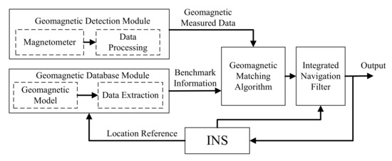
Figure 1.
Block diagram of geomagnetic matching-aided navigation system.
The ICCP algorithm realizes the alignment matching between the measured image and the model through the iteration of the closest point and takes the minimum Euclidean distance square as the objective function to obtain the optimal track between the measured track and the real track, so as to correct the measured track [14]. The principle of the algorithm is illustrated in Figure 2, where C (i = 1, 2, 3…N) is the magnetic field contour, P (i = 0, 1, 2, 3…N) is the inertial navigation indicating track sequence, Y (i = 1, 2, 3…N) is the matching target sequence, and X (i = 1, 2, 3…N) is the actual track sequence. The Euclidean distance of the objective function is minimized by the rigid transformation, and the algorithm ends until the objective function transformation is less than the threshold or reaches the maximum iteration times.
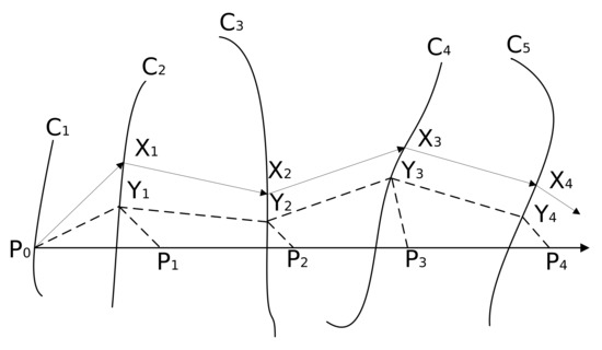
Figure 2.
Principle of ICCP algorithm.
The geomagnetic ICCP matching algorithm is based on the following two hypotheses.
Hypothesis 1.
The geomagnetic sensor has no measurement error.
Hypothesis 2.
The true position of the carrier is on the contour corresponding to the measured value of the magnetic field.
In practical applications, the sensor has inevitable errors, which cannot meet Hypothesis 1. In addition, when there is no adaptive area to choose from in the vehicle driving area, the ICCP algorithm caused by rigid transformation is easily affected by the accumulated errors of the inertial navigation system. As the increase of navigation time, the positioning error of each measuring point also increases, and the track indicated by inertial navigation gradually deviates from the real track. In these cases, if the Hypothesis 2 is not satisfied, the matching error of the iterative transformation using the ICCP algorithm will continue to increase. Therefore, it is necessary to study other methods to estimate the inertial navigation error, narrow the matching range, and obtain the approximate position of the AUV. Then, the ICCP matching algorithm is adopted to further improve the matching accuracy.
2.2. Vector Improved Algorithm for ICCP Matching
To satisfy the Hypothesis 2 of the ICCP matching algorithm, the traditional ICCP algorithm is improved in two aspects. First, the ACO algorithm is designed to amend the search strategy in a high probability range. Secondly, considering that the total geomagnetic features of the matching areas are very similar, the ICCP algorithm is prone to the problem of low matching accuracy or mismatch. And the terrain has only elevation information, while the geomagnetic field has abundant information features, such as vector features, three axes and seven components [15,16]. The objective function is improved by using the geomagnetic three-dimensional features, which is defined as the matching index. The specific improvements are reflected in the process of searching for areas and matching points.
2.2.1. Improvement of Search Area
The ICCP algorithm is a method to find the optimal alignment in global situation. The efficiency is relatively low because it searches the nearest point on the contour line in the whole map [17,18]. Considering the accumulated error of the INS, the upper and lower limits of error are added near the track indicated by the inertial navigation to limit the range, so that the real track is likely to fall in the area to be matched. The established search model is shown in Figure 3. The black dashed ellipse area is an error ellipse based on the coordinates indicated by the AUV.
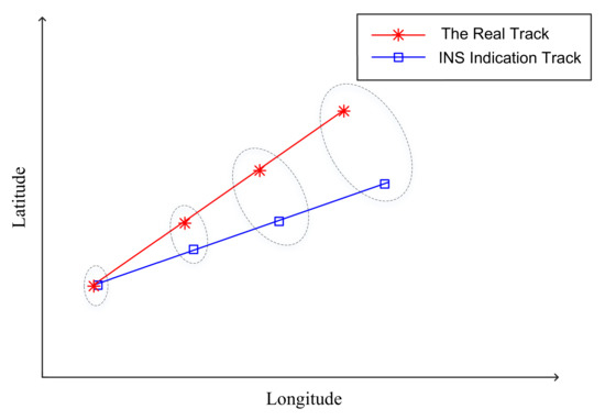
Figure 3.
Matching area with error.
Assuming that the positioning error of the INS obeys the standard normal distribution, are the east position variance, north position variance, and position covariance respectively, and is the standard deviation of the positioning error. The calculation formulas of the error ellipse are obtained by
where a is the semi-major axis of the ellipse, b is the semi-minor axis of the ellipse, and is the angle between the semi-major axis of the ellipse and the true north direction. According to the principle, when , the probability that the true track point falls within the error ellipse is 95%, and it can be considered that the matching is accurate within this range.
The essence of the matching navigation algorithm is the function optimization problem. As a classical simulation algorithm, the genetic algorithm refers to every possible solution as an individual, and uses a certain optimal rule, so that individuals can gradually reach the optimal solution through iteration [19]. The objective function is obtained by
where is the coordinate of the matching point, is the objective function corresponding to the point, N is the number of individuals, is the fitness of individual i, is the weighting factor corresponding to point . The purpose is to find the to maximize , and the corresponding is the estimated value of the position of the AUV.
The main function of the crossover operator is to create new individuals and realize the global search ability of the algorithm. From the perspective of the population evolution, the crossover probability should gradually decrease with the evolution process, and finally tend to a fixed value. From the perspective of the emergence of new individuals, all individuals in the population should have the same status, so the probability of genetic algorithm in search space is the same. Therefore, the crossover probability formula is obtained by
where is the population crossover probability of the t generation, t is the current evolution algebra, represents the maximum evolution algebra, is the maximum crossover probability, is the minimum crossover probability, and is an intermediate calculation variable.
The mutation operator mainly plays a role in maintaining the diversity of the population. The mutation probability of each individual in the same generation group varies with the strength of the individual. Therefore, the mutation probability of inferior individuals should be increased and the mutation probability of high-quality individuals reduced.Therefore, the following mutation probability formulas related to genetic evolution algebra and individual adaptation are obtained by
where is the mutation probability of individual in the t generation population, is the minimum mutation probability, is the maximum fitness value in the current population, is the maximum mutation probability, is the fitness value of the individual to be mutated.
Through the above strategy of narrowing the search area and updating the target point, the matching range is reduced to a suitable range, outlier points are eliminated continuously, high probability target points are increased, and matching efficiency is improved.
2.2.2. Improvements to Match Points
In a geomagnetic map where the total magnetic field does not change much, the ICCP algorithm uses the total magnetic field strength to perform translation and rotation transformations, which cannot clearly distinguish the real track and the inertial navigation indicated track, and it is easy to fall into mismatch. To solve this problem, when searching for the closest point, the three-component intensity of the geomagnetic field x, y and z is used as the evaluation index. According to the measured value of the magnetic field intensity on the real track sequence , the contour in the geomagnetic map is determined, and then the square sum of the difference between the three-component value of the magnetic field at each point on the contour and the three-component of the measuring point is calculated. Meanwhile, the smallest point in the sum of squares of the objective function difference is taken as the closest point on the contour, and finally the inertial navigation indicated sequence is rotated and translated, making the distance between the transformed path and the smallest. Repeat the above process until the algorithm converges or the accuracy is less than the threshold value.
When searching the closest point , the three-component intensity of x, y, and z is considered, and the physical index is obtained by
where , and are the magnetic field intensity in the x, y, and z directions corresponding to each point on the contour, respectively. , , and are the magnetic field strengths in the x, y, and z directions corresponding to the points on the real sequence.
The Hausdoff distance describes the similarity between two sets of points. It is used in the TERCOM matching algorithm, verifying the Hausdoff distance is more accurate than the Euclidean distance [20]. The calculation formula is obtained by
where and represent the one-way Hausdoff distance from to and to , respectively. The Hausdoff distance is used as the fitness to measure the closeness of the indicated track to the real track.
The process of the improved matching algorithm is as follows:
(1) Using B(i) as the matching index and the Hausdoff distance as the objective function, the ICCP algorithm is used to iteratively match the inertial navigation indication trajectory to obtain the estimated trajectory and determine the matching trajectory.
(2) Taking the estimated track as a benchmark, using Formulas (1)–(3) to make an error ellipse, an initial group consisting of N individuals is generated in the feasible region to delimit the initial matching area.
(3) Calculate fitness value. Take the of each individual and the measurement data sequence as the fitness value of the individual, select one half of the individuals with greater fitness to keep, and eliminate the points with larger errors in the population.
(4) Heredity and variation. Use Formulas (5)–(7) to update the fitness of the group and gradually move toward the optimal individual.
(5) Judging whether the termination conditions are satisfied. If not, go to step 2. If so, output the optimal solution.
3. Experiments
To verify the effectiveness of the improved ICCP matching algorithm based on the geomagnetic vector, the simulation experiment is performed. A certain sea area within the range of 38° to 38.1° north latitude and 120° to 120.15° east longitude is selected in this simulation. The total geomagnetic field strength in this range is illustrated in Figure 4. The grid spacing is 0.00125°, which is about 138.9 m.
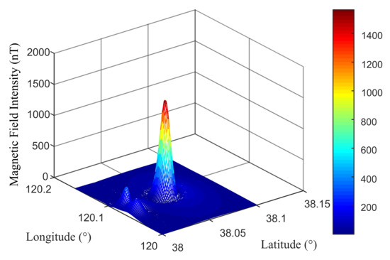
Figure 4.
Geomagnetic strength diagram.
Set the trajectory with an initial heading of 36.6 in the candidate matching area. The gyroscope of the inertial navigation system has a random drift with 0.04°/h and a constant drift with 0.04°/h. The accelerometer has a zero offset with 0.00005°/h and a random walk error with 0.00005°/h. The position error is ±10% of the measured value. Ten sampling points are selected on the trajectory, and the simulation matching result of the trajectory is shown in Figure 5 and the matching error is shown in Figure 6, which proves that the improved ICCP matching trajectory is closer to the real trajectory than the traditional ICCP matching trajectory.
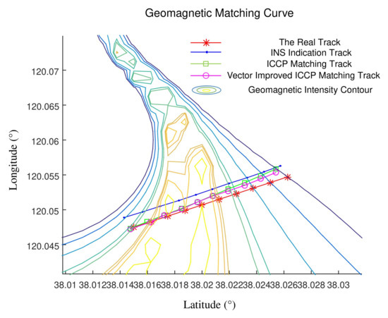
Figure 5.
Comparison of positioning result.
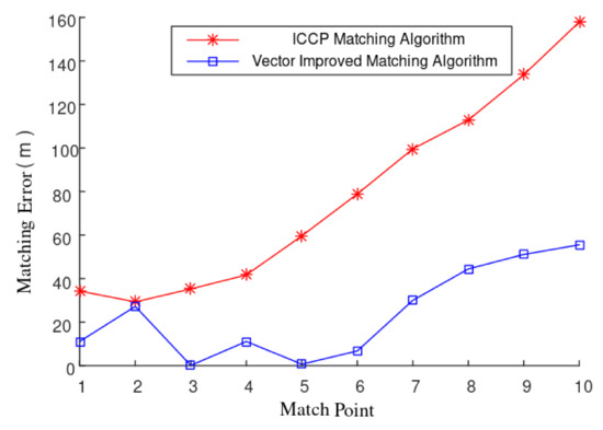
Figure 6.
Comparison of matching error.
The average positioning error, average heading error and matching time of the two ICCP matching algorithms are calculated, as shown in Table 1. According to the matching results, the vector improved ICCP algorithm can reduce the average position error from 783 m to 238 m, and the average heading error from 7.54° to 4.22°. According to the analysis of the algorithm implementation process, the vector improved ICCP algorithm replaces a large search area with an error ellipse, and the matching time is shortened from 15.62 s to 9.53 s. From the analysis of the algorithm implementation process, the vector improved ICCP algorithm replaces a large search area with an error ellipse, and the matching time is shortened from 15.62 s to 9.53 s.

Table 1.
Performance comparison of two ICCP algorithms.
The vector improved ICCP algorithm reduces the search range of the matching algorithm by improving the search area. Meanwhile, the ant colony algorithm accelerates the iterative update speed of the target point, and the matching time is reduced to 61.0% of the traditional ICCP algorithm, thus efficiency improving the matching efficiency. In addition, the matching index is optimized by combining the geomagnetic three-dimensional features and Hausdorff distance objective function. The results show that the position error is reduced to 30.4% and the heading error is reduced to 55.9% of the traditional algorithm, improving the matching accuracy. Therefore, the improved ICCP algorithm based on the geomagnetic vector can obtain a better matching effect.
4. Conclusions
Aiming at the problem that the ICCP algorithm is sensitive to heading error and easily mismatches in regions with similar geomagnetic general features, the ant colony algorithm is employed to improve the search area and process in the error ellipse, and the matching area is reduced, the outliers are continuously eliminated for target groups and the high probability points are added, so that the target can be converge quickly. The simulation results show the matching time is shortened to 61.0% of the original, and the matching efficiency is significantly increased. Combining the vector characteristics of geomagnetism, the three-axis components of the matching points are matched, and the Hausdoff distance is used to evaluate the fitness. This makes full use of the feature information of the target point, reducing the position error of the matching result to 30.4% and the heading error to 55.9% of the original, which improves the matching accuracy.
Author Contributions
Conceptualization, Y.R., L.W. and H.M.; methodology, Y.R., L.W., K.L., H.M. and M.M.; investigation, Y.R. and K.L.; writing—original draft preparation, Y.R., K.L., H.M. and M.M.; writing—review and editing, Y.R., K.L., H.M. and M.M.; supervision, L.W.; project administration, L.W. and H.M.; funding acquisition, L.W. and H.M. All authors have read and agreed to the published version of the manuscript.
Funding
This work was supported by State Key Laboratory of Geo-Information Engineering (NO. SKLGIE2019-K-2-1); National Natural Science Foundation of China (61773113).
Conflicts of Interest
The authors declare no conflict of interest.
References
- Paul, A.M.; Jay, A.F.; Zhao, F.; Vladimir, D. Autonomous Underwater Vehicle Navigation. IEEE J. Ocean. Eng. 2010, 35, 663–678. [Google Scholar]
- Tkhorenko, M.Y.; Pavlov, B.V.; Karshakov, E.V.; Volkovitsky, A.K. On integration of a strapdown inertial navigation system with modern magnetic sensors. In Proceedings of the Saint Petersburg International Conference on Integrated Navigation Systems, St. Petersburg, Russia, 28–30 May 2018; pp. 1–4. [Google Scholar]
- Liu, Z.; Zhang, L.; Liu, Q.; Yin, Y.; Cheng, L.; Zimmermann, R. Fusion of Magnetic and Visual Sensors for Indoor Localization: Infrastructure-Free and More Effective. IEEE Trans. Multimed. 2017, 19, 874–888. [Google Scholar] [CrossRef]
- Meng, W.; Jian, Y. Adaptive UKF-SLAM Based on Magnetic Gradient Inversion Method for Underwater Navigation; Springer: Cham, Switzerland, 2015. [Google Scholar]
- Liu, Z.; Chen, W.W.; Zhi-Gang, L.I. Return Navigation Algorithm Based on Magnetic Matching. J. Mil. Commun. Technol. 2016, 37, 80–84. [Google Scholar]
- Stateczny, A.; Blaszczak-Bak, W.; Sobieraj-Zlobinska, A.; Motyl, W.; Wisniewska, M. Methodology for Processing of 3D Multibeam Sonar Big Data for Comparative Navigation. Remote Sens. 2019, 11, 2245. [Google Scholar] [CrossRef] [Green Version]
- Zhang, T.; Li, Y.; Tong, J. An autonomous underwater vehicle positioning matching method based on iterative closest contour point algorithm and affine transformation. Proc. Inst. Mech. Eng. Part M J. Eng. Marit. Environ. 2017, 231, 711–722. [Google Scholar] [CrossRef]
- Wang, H.; Wu, L.; Chai, H.; Houtse, H.; Wang, Y. Technology of gravity aided inertial navigation system and its trial in South China Sea. IET Radar Sonar Navig. 2016, 10, 862–869. [Google Scholar] [CrossRef]
- Kang, C.; Wang, M.; Fan, L.; Zhang, X. Geomagnetic Navigation Region Selection Based on Geomagnetic Entropy and Geomagnetic Difference Entropy. J. Appl. Basic Eng. Sci. 2015, 23, 1156–1165. [Google Scholar]
- Quintas, J.; Teixeira, F.C.; Pascoal, A. An Integrated System for Geophysical Navigation of Autonomous Underwater Vehicles. IFAC-Pap. 2018, 51, 293–298. [Google Scholar] [CrossRef]
- Zhai, H.Q.; Wang, L.H. The robust residual-based adaptive estimation Kalman filter method for strap-down inertial and geomagnetic tightly integrated navigation system. Rev. Sci. Instrum. 2020, 91, 104501. [Google Scholar] [CrossRef] [PubMed]
- Chen, X.; Pang, Y.; Li, Y.; Chen, P. Underwater Terrain Matching Positioning Method Based on MLE for AUV. Robot 2012, 34, 559. [Google Scholar] [CrossRef]
- Wang, K.; Zhu, T.; Qin, Y.; Jiang, R.; Li, Y. Matching error of the iterative closest contour point algorithm for terrain-aided navigation. Aerosp. Sci. Technol. 2018, 73, 210–222. [Google Scholar] [CrossRef]
- Xiao, J.; Qi, X.; Duan, X. Research Status of Magnetic Matching Algorithm and Its Improvement Strategies. Electro-Opt. Control 2018, 25, 55–59. [Google Scholar]
- Zhou, L.; Cheng, X.; Zhu, Y.; Dai, C.; Fu, J. An Effective Terrain Aided Navigation for Low-Cost Autonomous Underwater Vehicles. Sensors 2017, 17, 680. [Google Scholar] [CrossRef] [PubMed] [Green Version]
- Zhai, H.; Wang, L.; Liu, Q.; Qiao, N. Geomagnetic signal de-noising method based on improved empirical mode decomposition and morphological filtering. Proc. Inst. Mech. Eng. Part G J. Aerosp. Eng. 2020, 33, 1–11. [Google Scholar] [CrossRef]
- Canciani, A.; John, R. Absolute Positioning Using the Earth’s Magnetic Anomaly Field. Navig.-J. Inst. Navig. 2016, 63, 111–126. [Google Scholar] [CrossRef]
- Afzal, M.H.; Renaudin, V.; Lachapelle, G. Magnetic field based heading estimation for pedestrian navigation environments. In Proceedings of the 2011 International Conference on Indoor Positioning and Indoor Navigation, Guimaraes, Portugal, 21–23 September 2011; pp. 1–10. [Google Scholar]
- Mo, R. Studying on comparison of different geomagnetic matching navigation algorithms. Geomat. Spat. Inf. Technol. 2016, 39, 46–48. [Google Scholar]
- Teixeira, F.-C.; Quintas, J.; Pascoal, A. Experimental validation of magnetic navigation of marine robotic vehicles. IFAC Pap. 2016, 49, 273–278. [Google Scholar] [CrossRef]
Publisher’s Note: MDPI stays neutral with regard to jurisdictional claims in published maps and institutional affiliations. |
© 2022 by the authors. Licensee MDPI, Basel, Switzerland. This article is an open access article distributed under the terms and conditions of the Creative Commons Attribution (CC BY) license (https://creativecommons.org/licenses/by/4.0/).