Article

Fully Automatic Analysis of Muscle B-Mode Ultrasound Images Based on the Deep Residual Shrinkage U-Net

College of Computer Science and Engineering, Shandong University of Science and Technology, Qingdao 266590, China
*
Author to whom correspondence should be addressed.
Electronics 2022, 11(7), 1093; https://doi.org/10.3390/electronics11071093
Submission received: 1 March 2022 / Revised: 22 March 2022 / Accepted: 29 March 2022 / Published: 30 March 2022
(This article belongs to the Special Issue Machine Learning in the Industrial Internet of Things)

Abstract

:
The parameters of muscle ultrasound images reflect the function and state of muscles. They are of great significance to the diagnosis of muscle diseases. Because manual labeling is time-consuming and laborious, the automatic labeling of muscle ultrasound image parameters has become a research topic. In recent years, there have been many methods that apply image processing and deep learning to automatically analyze muscle ultrasound images. However, these methods have limitations, such as being non-automatic, not applicable to images with complex noise, and only being able to measure a single parameter. This paper proposes a fully automatic muscle ultrasound image analysis method based on image segmentation to solve these problems. This method is based on the Deep Residual Shrinkage U-Net(RS-Unet) to accurately segment ultrasound images. Compared with the existing methods, the accuracy of our method shows a great improvement. The mean differences of pennation angle, fascicle length and muscle thickness are about 0.09°, 0.4 mm and 0.63 mm, respectively. Experimental results show that the proposed method realizes the accurate measurement of muscle parameters and exhibits stability and robustness.

1. Introduction

Muscle is an important tissue that constitutes part of the human body. It is densely distributed around organs and bones. Its function is to produce contractions and facilitate the body’s movement. According to its distribution and function, the human body’s muscle tissue can be divided into three categories: skeletal muscle, cardiac and smooth muscle. Skeletal muscle is attached to bones and accounts for about 40% of body weight. Its contraction and regulation have a great impact on the human body’s mobility, function and health [1]. Studies have shown that biological tissues’ mechanical properties and pathological changes are related to morphological changes. Therefore, the morphological information of skeletal muscle has a important reference value for disease diagnosis. Accurately quantifying changes in muscle structure parameters during exercise is of great significance to understanding muscle function and judging muscle state [2].
As a new method of non-contact sensing of lesions, ultrasound technology began to be used in medicine in the mid-1950s [3]. Initially, ultrasound technology was used in reproductive system imaging and fetal viability monitoring, such as heart valve motion imaging and abdominal organ imaging [4]. With the development of ultrasound imaging, it has been widely used in the diagnosis and treatment of many clinical diseases, such as skeletal muscle ultrasound images. Sonomyography (SMG) [5] is a method used to measure muscle morphologic parameters in ultrasound images. Muscle structure parameters can be easily obtained from the SMG, such as muscle thickness, pennation angle and the length of muscle fibers. The pennation angle reflects the axial torque of aponeuroses and its sub-torques. The changes in length of muscle fibers directly reflect muscle contraction, and the changes in muscle thickness demonstrate the position and state of the muscle. These dynamic or static muscle structure parameters [6] have important guiding significance for evaluating muscle function changes, muscle rehabilitation training and prosthetic control [7].
Since ultrasound imaging has been widely used in clinical medicine because of its painless, portable, and inexpensive features, the data interpretation of ultrasound images has always been a pivotal task. Traditionally, the quantitative parameters of skeletal muscle ultrasound images are manually measured or annotated using interactive software, but it is time-consuming, cumbersome and error-prone. Therefore, developing a convenient and accurate method for automatic measurement of muscle ultrasound images poses a new challenge. Recently, several methods of applying image processing technology to measure and quantify muscle ultrasound image parameters have emerged [8,9,10,11,12,13]. Zhao et al. [8] proposed an automatic linear extraction method based on local radon transformation (LRT) and rotation strategy to detect the pennation angle in ultrasound images. However, this method relies on the choice of edge detector. The measurement of images is often semi-automatic, and is not suitable for images containing different complex noises. Zhou et al. [12] combined the Gabor wavelet with the Hough transform, and used prior knowledge of the geometric arrangement of fascicles and aponeuroses in ultrasound images to realize the automatic measurement of pennation angle and muscle fiber length. Although this method performs well on images with high speckle noise, it lopsidedly relies on the parameterization of some features. The selection of parameters is empirical, and there are some uncertainties in practical application. Salvi et al. [13] proposed a method called MUSA to measure the muscle thickness on different ultrasound images of skeletal muscle. This method detects the fascicles in the middle of the aponeuroses through the Hough transform, and performs an iterative heuristic search on fascicles in the region of interest to identify contours of the aponeuroses and calculate muscle thickness. This feature detection method can locate the direction of representative fascicles. However, the speckle noise and the presence of intramuscular blood vessels tend to blur the critical features of muscle fibers, which will increase the difficulty of measurement. In addition, the MUSA method only measures the parameter of muscle thickness, which does not help to fully reflect the muscle state and structure. These image processing methods have initially solved the problem of data interpretation of muscle ultrasound images and performed well in accuracy. However, there are still various shortcomings that need to be further improved.
The advent of deep learning is undoubtedly attractive. It brings a new learning and prediction methods based on the inherent law of data. Deep learning methods have greatly improved the state of art in speech recognition, visual object recognition, object detection, and many other fields such as drug discovery and genomics [14]. The application of deep learning in various areas has also shown great potential in clinical medical research. Shen et al. [15] summarized the application of some deep generation models [16] in the medical field, such as deep belief networks (DBN) and deep Boltzmann machines (DBMs) and proposed that they have been successfully applied to brain disease diagnosis [17,18], lesion segmentation [19,20], cell segmentation [21] etc. This intelligent method can automatically acquire image features from ultrasound images through data training, effectively ’learning’ to recognize new images. Cunningham et al. [22] first used convolutional neural networks to analyze muscle structure. They proposed a model based on deep residual networks(Resnet) and convolutional neural networks (CNN) to measure the direction and curvature of human muscle fibers. After that, the method was further improved. The deconvolution and maximum deconvolution (DCNN) were used to quantify muscle parameters [23]. Through the comparison of various deep learning methods, the DCNN method was selected due to its remarkable muscle region localization ability. However, the difference of the pennation angle measured by this method is as high as 6 °, and there is still a lack of accuracy. Another automatic measurement method of the pennation angle based on deep learning has been proposed by Zheng et al [24]. In this method, a reference line is introduced to help detect the direction of muscle fibers, and a deep residual network determines the relative position of the line and muscle fibers. Then the pennation angle is calculated by adjusting the line until it is parallel to the fascicles. The results show that this method can accurately measure the pennation angle, but the measurement parameter is single and requires a large number of datasets to support it. With the development of image segmentation, the proposal of U-Net [25] makes medical image segmentation and recognition easier. J. Cronin et al. [26] constructed an ultrasonic image analysis method based on image segmentation using U-Net. The muscle parameters are obtained by calculating the segmentation results. We identify the DL method, which realizes the automatic measurement of muscle parameters. However, this method is cumbersome due to the separate training of two networks for aponeuroses and muscle fibers. When the image has complex noise, the measurement error rate is also high.
In general, there are some problems in the above methods: (1) the measurement method is not fully automatic. It relies on manual selection of filters or adjustment of preprocessing steps; (2) the measurement results are not ideal for ultrasound images with complex noises; (3) it is difficult to obtain all the essential parameters in muscle ultrasound images solely by one method, which is not conducive to a comprehensive analysis of muscle status.
In this study, in order to amend the limitations of above methods, we propose a method with an improved neural network structure based on U-Net and deep residual shrinkage networks (DRSN), called RS-Unet, for accurate segmentation of muscle ultrasound images. Firstly, the manually labeled datasets are input into the model for training, and the trained model is used to segment the muscle ultrasound images to obtain clear and accurate results. On this basis, the segmentation results are further processed, aponeuroses and muscle fibers are linearly fitted, and the intersection points are calculated. Finally, the structure parameters of muscle ultrasound images are accurately measured, including muscle thickness, pennation angle and fascicle length. The method we proposed is a fully automatic muscle parameter detection method without any manual preprocessing steps. Experimental results show that our method produced similar results to the manual method, and has good performance in automatic and accurate measurement of muscle parameters.
The main contributions of this study are as follows:
  • We analyzed the existing muscle ultrasound image analysis methods, including those using image processing technology and deep learning technology, and summarized their advantages and limitations.
  • We propose a fully automatic muscle ultrasound image analysis method based on RS-Unet. It can analyze muscle ultrasound images with complex noise more accurately without any manual preprocessing. The parameters of muscle thickness, pennation angle and fascicle length can be easily calculated.
  • A new network model called RS-Unet is proposed for muscle ultrasound image segmentation. It is stable and robust. In the future, it has the potential to be applied in other ultrasonic image analysis fields.
The remaining parts of this study are as follows. In section two, we introduce the specific research methods. Section three is the experimental study of our proposed method on muscle ultrasound images. Section four is the discussion and comparison of experimental results. Section five summarizes the whole paper.

2. Materials and Methods

In our method, the processing process of a muscle ultrasound image is divided into two modules shown in Figure 1. In the training module, manually labeled dataset is input into our neural networks for training, and the optimal model is obtained. In the segmentation and calculation module, the ultrasound image without any preprocessing is entered into the trained model, and the results of segmentation are obtained. The segmentation results are then subjected to a series of post-processing, including contour extraction, line fitting, and calculation of intersection points. Finally, the length of muscle fibers, pennation angle and muscle thickness are calculated. The accurate measurement of this method is based on the precise segmentation of RS-Unet, and the network structure of RS-Unet will be described in detail below.

2.1. Network Architecture of RS-Unet

Our proposed network structure is called Deep Residual Shrinkage U-Net (RS-Unet), which is an improved neural networks model based on the design idea of U-Net and combined with the deep residual shrinkage networks. Figure 2 shows the architecture of RS-Unet. The U-Net is a neural network model proposed by Ronneberge et al. [25] in 2015 for medical image segmentation tasks. It consists of an encoder and a decoder with the same number of convolutions. The down-sampling of the encoder is used to extract the semantic information of the image, and the up-sampling of the decoder restores the size of image. The skip connection between the up-sampling layer and the down-sampling layer helps to recover the detailed information of the image, but will also send some noise or useless information to the decoder and negatively affect the final segmentation result. Therefore, although U-Net achieved some results in many fields including medical image segmentation, it is difficult to achieve desirable results in the face of such a complex task as muscle ultrasound image segmentation. To solve this problem, we propose RS-Unet, which uses residual shrinkage blocks instead of the traditional convolutional blocks in the encoder. While deepening the network and expanding the receptive field through the structure of residuals, the attention mechanism and soft thresholding is introduced into the residual block to form the residual shrinkage block, which enhances the feature extraction ability and suppresses the noise.
The large size images of 512 × 512 are selected as the input, which is different from the methods of inputting small images for neural networks training fast. Because muscle ultrasound images are generally blurred and the quality of images is poor, a larger size of images avoids the loss of pixel information in the down-sampling layers, so as to ensure more accurate segmentation. As shown in Figure 2, each unit in the encoder includes a residual shrinkage block for extracting image features and a down-sampling layer which uses a max-pooling of 2 × 2 to reduce the feature map size by half. The decoder is the same as the standard U-Net, and the feature map is restored to the original size through multiple 3 × 3 deconvolutions. The deconvolution is essentially transposed convolution, which was proposed by Zeiler [27] in 2010. The feature fusion of the RS-Unet is in a typical U-Net fashion by skip connection. It transmits feature information by clipping and splicing the same level feature maps of encoder and decoder. It enables spatial information to be directly applied to deeper layers to obtain more accurate segmentation results. The skip connection in RS-Unet adopts direct splicing without clipping, which preserves the edge information of the image as much as possible. In the last layer, the feature map passes through a softmax function to output a three-channel mask. Each channel corresponds to a different pixel classification, which are muscle fibers, aponeuroses and background. Because each pixel in the mask represents the probability of each classification. The channel with the maximum probability value is selected by the threshold, which ensures the accuracy and clear of segmentation results.

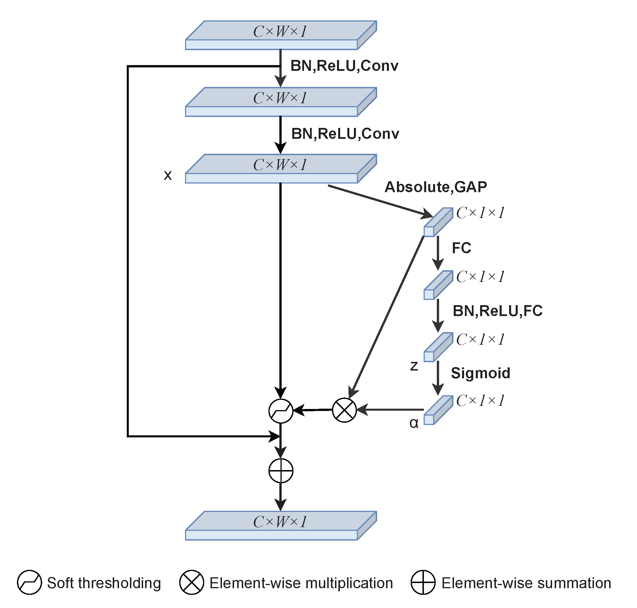
2.2. Deep Residual Shrinkage Block

At each level of the RS-Unet encoder, the feature map goes through a residual shrinkage block. It is a part of the Deep Residual Shrinkage Networks (DRSN). It was proposed by Zhao et al. [28] as a variant of Deep Residual Networks (ResNet) that uses soft thresholding to remove noise-related features. Soft thresholding is often used as a key step in many signal denoising methods [29,30]. It is a function that reduces the input data to near zero. It removes the features whose absolute value is less than a certain threshold and makes the features whose absolute value is greater than this threshold shrink to near zero. Soft thresholding is defined as follows:
y = x τ x > τ 0 τ x τ x + τ x < τ
where x is the input feature, y is the output feature, and τ is the threshold. The derivative of the soft thresholded output with respect to the input is:
y x = 1 x > τ 0 τ x τ 1 x < τ
It can be observed that the derivative of output to input is 1 or 0, which can reduce the risk of the deep learning algorithm encountering gradient disappearance and explosion.
The setting of the threshold in soft thresholding of the deep residual shrinkage networks is different from that in signal processing. The threshold will be automatically learned in deep learning without the need for experts to set it manually. Figure 3 shows the structure diagram of the residual shrinkage block. First, the input is convolved twice to obtain feature map x. In the special module, the feature map is compressed using global average pooling (GAP) to obtain a set of one-dimensional vectors (that is, a set of channel weights are learned). The one-dimensional vectors are passed through two FC layers to obtain a set of scaling parameters. The output of the FC network is scaled to the range (0,1) using:
α c = 1 1 + e z c
z c is the feature map of the cth neuron output by the FC network, and α c is the cth scaling parameter. The next step is to calculate the threshold:
τ c = α c · 1 w × h i = 1 w j = 1 h | x i , j , c |
τ c is the threshold of the cth channel of the feature map, h, w, c are the indexes of width, height and channels of the feature map x. Through soft thresholding, the features irrelevant to the current task are set to 0, and the features relevant to the current task are retained, thus realizing the suppression of noise. Compressing to the channel domain for convolution enhances the learning ability of the channel features and improves the extraction ability of the model for important features. The DRSN also retains the characteristics of ResNet [22]. The residual learning structure is realized by shortcut connection, which performs the equivalent mapping and solves the problem of network degradation in the process of network layer deepening.

2.3. Loss Function

The outputs of RS-Unet are the result of three classifications (fascicles, aponeuroses and background), which is actually a process of classifying pixels as samples. Segmentation networks typically use a cross-entropy (CE) function as a loss function. Still, due to the number of samples of muscle fibers and aponeuroses being small in ultrasound images, sample imbalance is severe. The dice loss function was proposed by Fausto Milletari et al. [31] in the paper of VNet, which is used to solve the problem of sample imbalance in image segmentation. Therefore, to focus on the characteristics of muscle fibers and aponeuroses during model training, dice loss function should be used in each dimension:
L d i c e = 1 1 m j = 1 m 2 i = 1 N y i j y ^ i j i = 1 N y i j + i = 1 N y ^ i j
where y i j is the true probability value for each pixel, y ^ i j represents the predicted probability value, N is the total number of pixels, and m represents the class (fascicles, aponeuroses and background).

3. Results

3.1. Datasets

We collected ultrasound image datasets from different types of movements conducted by different groups of the population (including young people, elderly people, etc.). These data include a large number of videos and images, which are obtained from muscle tissues in different parts of the body (medial and lateral gastrocnemius, vastus lateralis, tibialis anterior) using a variety of ultrasound devices.To ensure the diversity of data, we collected data from different sources. Some of these were collected by experts from Shenzhen Institute of advanced research, Chinese Academy of Sciences, and some are from the research of J. Cronin et al. [26]. A set of 508 samples was obtained by cutting images and randomly extracting videos by frame. Three researchers used FIJI software [32] to manually label the dataset to generate masks. Each mask is divided into three parts with different colors, with the blue part representing muscle fibers, the red representing aponeuroses, and the green representing background. Figure 4 shows the samples of the manually labeled dataset. The dataset is divided into a training set and a validation set according to the ratio of 9:1. Another 50 samples are randomly selected from the videos besides the training set to form a test dataset, which ensures the reliability of experiment results. These data have received ethical approval from the relevant committees of Shenzhen Institutes of Advanced Technology, CAS.

3.2. Details and Training

The experiments utilize a Tesla P100 GPU with 128GB of memory for model training. The images of the training dataset were adjusted to 512 × 512 size to feed the network, which can avoid the loss of important features. Python was used to run the codes of the experiment, and the deep learning framework was TensorFlow 1.4.0. The Adam optimizer iswas applied to optimize experimental parameters while iteratively adjusting the learning rate. The batch size of the training was set to 4, and 93 epochs were trained totally.
When the training loss of model decreases and the test loss remains unchanged or increases, that is, the overfitting phenomenon occurs, the training will be stopped in advance. To obtain the optimal model, we trained on datasets of different sizes. The three sizes of data set with 208, 358 and 508 images were chosen, respectively. The loss function of training was calculated using the dice loss function in Equation (5). Figure 5a,b shows the loss curves and accuracy curves of the training dataset and the validation dataset with different sizes of data set. The results show that the model performs better when the size of data set is 508. Complex network models need larger data sets for training to achieve higher accuracy. Too small data sets, such as those containing 208 pictures, shown in Figure 5, may lead to over fitting of the model. However, the data set with too large an amount of data will also contain more noise. So, choosing an appropriate size of data set is important for training. Through training with 508 images, the training loss and verification loss of the model decrease continuously until they become stable, and the accuracy rate is high, indicating that the model training process is successful.

3.3. Segmentation results

Figure 6 shows some segmentation results of the model. It can be seen that the aponeuroses and muscle fibers are well identified and segmented, and the noise and blur are also successfully suppressed. The model performs well in segmenting ultrasound images of muscles with different parts of body and with different noises. As shown in Figure 6d, even though the noise in the image is still conspicuous, aponeuroses and parts of muscle fibers can still be successfully segmented, which is enough to accurately calculate the muscle structure parameters in the post-processing step. This result is undoubtedly gratifying.

3.4. Post-Processing

After obtaining the segmentation results of the model, images require a series of post-processing to calculate parameters such as muscle thickness. The following processing is implemented by OpenCv. First, contours of the deep and superficial aponeuroses and fascicles are extracted (Figure 7a). The upper and lower edges of the aponeurosis contours close to fascicles are fitted into a line (Figure 7b). Long fascicles are more accurate and can represent the overall direction of muscle fibers, while the short fascicles are often affected by noise. We selected the 10 fascicles with the longest contours for calculation (Figure 7c). The fascicles were fitted into lines and extended, and intersection points of the fascicles, along with aponeuroses, were calculated. The length and pennation angle of muscle fibers were calculated by taking the average of 10 fascicles (Figure 7d). The muscle thickness is represented by the width at middle of overlapping part of the deep and superficial aponeuroses. The algorithms for calculating muscle thickness, pennation angle and fascicle length are described in Algorithm 1 and Algorithm 2, respectively. Figure 8 shows the final results of post-processing. In order to intuitively display the parameter results, we directly show the parameters in the figure.
  • Algorithm 1 Calculating the muscle thickness.
  • Input: Segmentation result from the model, i m a g e ;
    Output: muscle thickness;
    •  1: Init L c = a p p r o p r i a t e t h r e s h o l d ;
    •  2: Extract the contours of aponeuroses in i m a g e , C = { c 1 , c 2 , . . . , c n } ;
    •  3: Choose the length of contours > L c in C as C , C = { c 1 , c 2 } ;
    •  4: Sort the two contours in C according to the Y coordinates, S o r t C = { s c 1 , s c 2 } ;
    •  5: Obtain the lower boundary of s c 1 and fit it into a line, l 1 ; obtain the upper boundary of s c 2 and fit it into a line, l 2 ;
    •  6: Select three equally divided points in the middle on l 1 , p 1 , p 2 , p 3 ;
    •  7: Calculate the mean of the distance from p 1 , p 2 , p 3 to l 2 as the muscle thickness;
    •  8: return muscle thickness;
  • Algorithm 2 Calculating the pennation angle and fascicle length.
  • Input: Segmentation result from the model, i m a g e ;
  • Output: pennation angle and fascicle length;
    •  1: Extract the contours of fascicles in i m a g e , F = { f 1 , f 2 , . . . , f n } ;
    •  2: Select the longest 10 contours in F as F , F = { f 1 , f 2 , . . . , f 10 } ;
    •  3: Fit each contour in F into a straight line;
    •  4: Extend each line to intersect l 1 and l 2 in A l g o r i t h m 1 ;
    •  5: Calculate the mean length between the intersections of 10 lines as fascicle length;
    •  6: Calculate the mean of angles at the intersection as pennation angle;
    •  7: return pennation angle, fascicle length;

4. Discussion

In this section, we evaluate the proposed model and method through a series of experiments, including the analysis and comparison of models and the discussion of prediction results. By comparing the segmentation results of different models and the influence of different network designs on the segmentation outcomes, the effectiveness and the robustness of our model are demonstrated. The parameter results of our proposed method and the existing DL method [26] on manually labeled test datasets are used for parameter results comparison.

4.1. Analysis of the Network Model

To study the effect of the structure of the proposed model, an ablation experiment was used for discussion. As shown in Table 1, we compared the impact of shrinkage on model performance. Experiments show that the shrinkage structure has a positive impact on the performance of RS-Unet and can increase the accuracy of segmentation results. This is because the residual shrinkage block takes soft thresholding as shrinkage function, and discriminant features can be learned through a variety of nonlinear transformations to eliminate the noise-related information. The research on thresholding is shown in Table 2.
We compared the impact of the model with soft thresholding and hard thresholding, respectively. Hard thresholding is also a common denoising method in signal processing. The calculation of this is as follows:
H a r d ( x , τ ) = x | x | > τ 0 | x | < = τ
where x is the input feature and τ is the threshold. The results in Table 2 show that replacing the soft thresholding in the residual shrinkage block with hard thresholding makes the performance parameters worse. Soft thresholding can eliminate complex noise, retain the features with thresholds close to zero and make the segmentation results more precise.
To discuss the performance of RS-Unet, we use the same data set to input different models. The data set includes 508 samples, of which 51 samples are used as a validation dataset. Table 3 shows an evaluation of models on U-Net [25], ResU-Net [33], RS-CBAM-Unet and RS-Unet. The accuracy, IoU, DSC, precision, recall and F-score were used as the performance measures of the proposed model. They are calculated as follows:
D S C = 2 | X Y | | X | + | Y | = 2 T P 2 T P + F P + F N
I o U = | X Y | | X | + | Y | | X Y | = T P T P + F P + F N
P = T r u e p o s i t i v e s p r e d i c t e d a s p o s i t i v e = T P T P + F P
R = T r u e p o s i t i v e s a c t u a l p o s i t i v e s = T P T P + F N
F s c o r e = 2 × P × R P + R
where, P represents precision, R represents recall, and F s c o r e is the harmonic mean of the two, which is between zero and one. The closer it is to one, the better the result. The X is the ground truth, and Y is the predicted area output by the model. Table 3 shows that the segmentation result of RS-Unet is more accurate. The performance of the model has been improved.
As shown in Table 3, the performance of RS-Unet has been improved. Compared with other models, each performance measure has been improved to varying degrees.The RS-CBAM-Unet mentioned in Table 3 is a model formed by adding a Convolutional Block Attention Module (CBAM) in the middle part of the RS-Unet. CBAM is a mixed attention module proposed by Woo et al. [34] in 2018, which improves the learning ability of important features through channel and spatial attention. This module performs well in classification and regression models, but has not been applied to segmentation models. According to the experiment, after adding this module, the performance of the model has not been improved. On the contrary, its accuracy is lower than RS-Unet. This is due to the fact that the significance of channel information is much higher than that of spatial information for the segmentation networks we designed. The CBAM may cause the loss of important channel information originally obtained in the compression process by trying to obtain spatial attention. In our application, the spatial attention did not promote the segmentation of samples. Moreover, the number of parameters of RS-CBAM-Unet has increased drastically, and the loss of the model is also higher than that of RS-Unet, which is 0.29. Therefore, we eventually chose the RS-Unet without CBAM.
We visualized the segmentation results of the samples to observe the effect of different models. Figure 9 shows some segmentation results of the four models. The first column is the original muscle ultrasound image, the second, third, fourth and fifth columns are the segmentation results output from the four models, and the sixth column is the ground truth annotated by researchers. Although all the models realize the segmentation to images, the proposed network model shows more accuracy and robustness in detail. It also performs well in the case of complex noise and low contrast. The identification of aponeuroses is more coherent, and muscle fibers are clearer. In general, the proposed model can segment muscle ultrasound images more precisely, which is essential for post-processing and accurate acquisition of quantitative parameters.

4.2. Analysis of Methods

To validate the proposed method, We used another group of gastrocnemius ultrasound videos to randomly intercept 50 images by frame as the test dataset. We compare the experimental results with the DL method and manual method. The DL method trained two models to identify aponeuroses and muscle fibers, respectively. The segmentation results of models are shown in Figure 10. In Figure 10b, due to the influence of noise, the DL method is not accurate enough to segment aponeuroses, and many background noises are mistaken for aponeuroses. The segmentation result of muscle fibers is shown in Figure 10c. The feature extraction ability is not strong enough, so the segmentation of muscle bundle is crude. In contrast, the segmentation result of our method is clearer and more accurate. As shown in Figure 10d, when the edges of aponeuroses are not clear and muscle fibers are easily confused with noise, our method can better avoid the influence of noise.
The quantitative parameters of the muscle ultrasound images are obtained by post-processing. In order to further validate the effectiveness of our proposed method, we compare the results of parameters with the DL method and the manual method. As a classic consistency evaluation method, Bland–Altman plots [35] were proposed in 1986. In our experiment, they were used to analyze the consistency between the two methods and the manual method. The 50 images of the test dataset were labeled by three researchers, respectively. Figure 11 shows the Bland–Altman plots of the DL method and our method with the manual method by the first researcher. The abscissa is the mean value of two methods, and the ordinate is the mean difference of the measurement results. The solids indicate the mean of the differences, and the dashed lines represents the 95% agreement limit of the mean difference ± 1.96 standard deviation (SD). Figure 11a,c,e is the consistency analysis of the muscle parameters measured by our method and the manual method. The results of our method are almost between the 95% consistency bounds, which proves that our method is in good agreement with the manual method. Moreover, the mean differences in the pennation angle, muscle fiber length, and muscle thickness between our method and manual method were 0.09°, 0.4 mm and 0.63 mm, respectively. The results were less than the mean difference of 0.14°, 0.9 mm and 0.67 mm between the DL method and the manual method, as shown in Figure 11b,d,f, respectively. In order to reduce the subjective factors and make the experiment more convincing, the two methods were compared with the ground truth labeled by two other researchers. The standard deviation (SD), root mean square errors (RMSEs), 95% agreement bounds for the DL method and our method are shown in Table 4.
In Table 4, pennation means the pennation angle, length means the muscle fiber length, and thickness means muscle thickness. The RMSEs represent the difference between the predicted value and the true value, and the analysis of the results shows that the RMSEs of our method are smaller than that of the DL method. The SD shows the difference between the results and means; our results are less different from the mean, and the 95% agreement bound interval is also smaller. In general, the results of our method are closer to those obtained by manual labeling and better than those obtained by the DL method. This is due to the better performance of the RS-Unet, and the seletion of long muscle fibers in post-processing. It reduces the influence of noise and ensures the robustness of our method.
As a fully automatic measurement method, the advantage of DL method is that it can measure three important muscle parameters accurately. However, its precision is high not enough and it does not perform well in the case of high noise. Compared with DL and other existing methods, our method can automatically and comprehensively measure muscle parameters. The accuracy of measurement and segmentation is also higher. It uses a model that removes some noise and enhances feature learning, making also it applicable to high-noise muscle ultrasound images.
Although our method achieves automatic analysis of muscle ultrasound images accurately, there are still some limitations. Due to the suppression of noise by soft thresholding, there may be an obstacle tosome muscle fiber recognition in images with high noise intensity and very blurred muscle fibers. In the future, we will try to use an attention mechanism and other methods to solve this problem. In addition, our method approximately fits the muscle fibers into straight lines. If the muscle fibers are severely curved in a part of the ultrasound image, our prediction results may not be accurate enough. In future research, we will further improve the proposed method, such as focusing on the analysis of muscle ultrasound videos and the identification of different kinds of muscle tissue.

5. Conclusions

In this paper, we propose an automatic method to analyze muscle ultrasound images based on image segmentation. In this method, the RS-Unet is used to segment images, and after post-processing and calculation, the accurate measurement of quantitative parameters of muscle ultrasound images is realized. The RS-Unet model is a new neural network model, which uses the residual shrinkage blocks instead of convolution blocks in U-Net to enhance the ability of feature extraction and noise suppression. The dice loss function is used to replace the cross-entropy function to solve the problem of unbalanced samples of muscle fibers, aponeuroses and background. In terms of model performance, compared with U-Net and other improved networks, the IoU and dice coefficients of our model show significant improvements, and it works well in the visualization of segmentation results. In terms of parameter prediction, we compared our results with the DL method using the dataset manually labeled by three researchers. Our results were in good agreement with the manual method, and the accuracy of our results was also better than that of the DL method. Experiments show that our proposed method can achieve accurate segmentation of muscle ultrasound images and the accurate prediction of parameters. It is stable and robust enough to perform well in the case of complex noise.

Author Contributions

Conceptualization, W.Z., L.Z. and S.L.; methodology, L.Z.; validation, L.Z.; formal analysis, S.L.; resources, W.Z. and S.L.; funding acquisition, W.Z.; writing—original draft preparation, L.Z.; writing—review and editing, W.Z., Q.C. and J.X. All authors have read and agreed to the published version of the manuscript.

Funding

This project was funded by National Natural Science Foundation of China [Grant No.11974373].

Conflicts of Interest

The authors declare no conflict of interest.

References

  1. Frontera, W.R.; Ochala, J. Skeletal muscle: A brief review of structure and function. Calcif. Tissue Int. 2015, 96, 183–195. [Google Scholar] [CrossRef]
  2. Yuan, C.; Chen, Z.; Wang, M.; Zhang, J.; Sun, K.; Zhou, Y. Dynamic measurement of pennation angle of gastrocnemius muscles obtained from ultrasound images based on gradient Radon transform. Biomed. Signal Processing Control 2020, 55, 101604. [Google Scholar] [CrossRef]
  3. Nicolson, M.; Fleming, J.E. Imaging and Imagining the Fetus: The Development of Obstetric Ultrasound; JHU Press: Baltimore, MD, USA, 2013. [Google Scholar]
  4. Havlice, J.F.; Taenzer, J.C. Medical ultrasonic imaging: An overview of principles and instrumentation. Proc. IEEE 1979, 67, 620–641. [Google Scholar] [CrossRef]
  5. Zheng, Y.P.; Chan, M.; Shi, J.; Chen, X.; Huang, Q.H. Sonomyography: Monitoring morphological changes of forearm muscles in actions with the feasibility for the control of powered prosthesis. Med. Eng. Phys. 2006, 28, 405–415. [Google Scholar] [CrossRef] [Green Version]
  6. Cronin, N.J.; Lichtwark, G. The use of ultrasound to study muscle–tendon function in human posture and locomotion. Gait Posture 2013, 37, 305–312. [Google Scholar] [CrossRef]
  7. Guo, J.Y.; Zheng, Y.P.; Xie, H.B.; Koo, T.K. Towards the application of one-dimensional sonomyography for powered upper-limb prosthetic control using machine learning models. Prosthetics Orthot. Int. 2013, 37, 43–49. [Google Scholar] [CrossRef] [Green Version]
  8. Zhao, H.; Zhang, L.Q. Automatic tracking of muscle fascicles in ultrasound images using localized radon transform. IEEE Trans. Biomed. Eng. 2011, 58, 2094–2101. [Google Scholar] [CrossRef]
  9. Zhou, Y.; Zheng, Y.P. Estimation of muscle fiber orientation in ultrasound images using revoting hough transform (RVHT). Ultrasound Med. Biol. 2008, 34, 1474–1481. [Google Scholar] [CrossRef] [Green Version]
  10. Namburete, A.I.; Rana, M.; Wakeling, J.M. Computational methods for quantifying in vivo muscle fascicle curvature from ultrasound images. J. Biomech. 2011, 44, 2538–2543. [Google Scholar] [CrossRef]
  11. Cronin, N.J.; Carty, C.P.; Barrett, R.S.; Lichtwark, G. Automatic tracking of medial gastrocnemius fascicle length during human locomotion. J. Appl. Physiol. 2011, 111, 1491–1496. [Google Scholar] [CrossRef]
  12. Zhou, G.Q.; Chan, P.; Zheng, Y.P. Automatic measurement of pennation angle and fascicle length of gastrocnemius muscles using real-time ultrasound imaging. Ultrasonics 2015, 57, 72–83. [Google Scholar] [CrossRef]
  13. Caresio, C.; Salvi, M.; Molinari, F.; Meiburger, K.M.; Minetto, M.A. Fully automated muscle ultrasound analysis (MUSA): Robust and accurate muscle thickness measurement. Ultrasound Med. Biol. 2017, 43, 195–205. [Google Scholar] [CrossRef]
  14. LeCun, Y.; Bengio, Y.; Hinton, G. Deep learning. Nature 2015, 521, 436–444. [Google Scholar] [CrossRef]
  15. Shen, D.; Wu, G.; Suk, H.I. Deep learning in medical image analysis. Annu. Rev. Biomed. Eng. 2017, 19, 221–248. [Google Scholar] [CrossRef] [Green Version]
  16. Salakhutdinov, R. Learning deep generative models. Annu. Rev. Stat. Its Appl. 2015, 2, 361–385. [Google Scholar] [CrossRef] [Green Version]
  17. Suk, H.I.; Lee, S.W.; Shen, D.; Alzheimer’s Disease Neuroimaging Initiative. Hierarchical feature representation and multimodal fusion with deep learning for AD/MCI diagnosis. NeuroImage 2014, 101, 569–582. [Google Scholar] [CrossRef] [Green Version]
  18. Suk, H.I.; Wee, C.Y.; Lee, S.W.; Shen, D. State-space model with deep learning for functional dynamics estimation in resting-state fMRI. NeuroImage 2016, 129, 292–307. [Google Scholar] [CrossRef] [Green Version]
  19. Dou, Q.; Chen, H.; Yu, L.; Zhao, L.; Qin, J.; Wang, D.; Mok, V.C.; Shi, L.; Heng, P.A. Automatic detection of cerebral microbleeds from MR images via 3D convolutional neural networks. IEEE Trans. Med. Imaging 2016, 35, 1182–1195. [Google Scholar] [CrossRef]
  20. Brosch, T.; Tang, L.Y.; Yoo, Y.; Li, D.K.; Traboulsee, A.; Tam, R. Deep 3D convolutional encoder networks with shortcuts for multiscale feature integration applied to multiple sclerosis lesion segmentation. IEEE Trans. Med. Imaging 2016, 35, 1229–1239. [Google Scholar] [CrossRef]
  21. Roux, L.; Racoceanu, D.; Loménie, N.; Kulikova, M.; Irshad, H.; Klossa, J.; Capron, F.; Genestie, C.; Le Naour, G.; Gurcan, M.N. Mitosis detection in breast cancer histological images An ICPR 2012 contest. J. Pathol. Inform. 2013, 4, 8. [Google Scholar] [CrossRef]
  22. Cunningham, R.; Harding, P.; Loram, I. Deep residual networks for quantification of muscle fiber orientation and curvature from ultrasound images. In Proceedings of the Annual Conference on Medical Image Understanding and Analysis, Edinburgh, UK, 11–13 July 2017; Springer: Cham, Switzerland, 2017; pp. 63–73. [Google Scholar]
  23. Cunningham, R.; Sánchez, M.B.; May, G.; Loram, I. Estimating full regional skeletal muscle fibre orientation from B-mode ultrasound images using convolutional, residual, and deconvolutional neural networks. J. Imaging 2018, 4, 29. [Google Scholar] [CrossRef] [Green Version]
  24. Zheng, W.; Liu, S.; Chai, Q.W.; Pan, J.S.; Chu, S.C. Automatic Measurement of Pennation Angle from Ultrasound Images using Resnets. Ultrason. Imaging 2021, 43, 74–87. [Google Scholar] [CrossRef]
  25. Ronneberger, O.; Fischer, P.; Brox, T. U-Net: Convolutional networks for biomedical image segmentation. In Proceedings of the International Conference on Medical Image Computing and Computer-Assisted Intervention, Munich, Germany, 5–9 October 2015; Springer: Cham, Switzerland, 2015; pp. 234–241. [Google Scholar]
  26. Cronin, N.J.; Finni, T.; Seynnes, O. Fully automated analysis of muscle architecture from B-mode ultrasound images with deep learning. arXiv 2020, arXiv:2009.04790. [Google Scholar]
  27. Zeiler, M.D.; Krishnan, D.; Taylor, G.W.; Fergus, R. Deconvolutional networks. In Proceedings of the 2010 IEEE Computer Society Conference on Computer Vision and Pattern Recognition, San Francisco, CA, USA, 13–18 June 2010; pp. 2528–2535. [Google Scholar]
  28. Zhao, M.; Zhong, S.; Fu, X.; Tang, B.; Pecht, M. Deep residual shrinkage networks for fault diagnosis. IEEE Trans. Ind. Inform. 2019, 16, 4681–4690. [Google Scholar] [CrossRef]
  29. Donoho, D.L. De-noising by soft-thresholding. IEEE Trans. Inf. Theory 1995, 41, 613–627. [Google Scholar] [CrossRef] [Green Version]
  30. Isogawa, K.; Ida, T.; Shiodera, T.; Takeguchi, T. Deep shrinkage convolutional neural network for adaptive noise reduction. IEEE Signal Processing Lett. 2017, 25, 224–228. [Google Scholar] [CrossRef]
  31. Milletari, F.; Navab, N.; Ahmadi, S.A. V-net: Fully convolutional neural networks for volumetric medical image segmentation. In Proceedings of the 2016 Fourth International Conference on 3D Vision (3DV), Stanford, CA, USA, 25–28 October 2016; pp. 565–571. [Google Scholar]
  32. Schindelin, J.; Arganda-Carreras, I.; Frise, E.; Kaynig, V.; Longair, M.; Pietzsch, T.; Preibisch, S.; Rueden, C.; Saalfeld, S.; Schmid, B.; et al. Fiji: An open-source platform for biological-image analysis. Nat. Methods 2012, 9, 676–682. [Google Scholar] [CrossRef] [Green Version]
  33. Diakogiannis, F.I.; Waldner, F.; Caccetta, P.; Wu, C. ResUNet-a: A deep learning framework for semantic segmentation of remotely sensed data. ISPRS J. Photogramm. Remote Sens. 2020, 162, 94–114. [Google Scholar] [CrossRef] [Green Version]
  34. Woo, S.; Park, J.; Lee, J.Y.; Kweon, I.S. Cbam: Convolutional block attention module. In Proceedings of the European Conference on Computer Vision (ECCV), Munich, Germany, 8–14 September 2018; pp. 3–19. [Google Scholar]
  35. Bland, J.M.; Altman, D. Statistical methods for assessing agreement between two methods of clinical measurement. Lancet 1986, 327, 307–310. [Google Scholar] [CrossRef]
Figure 1. Processing flow of the proposed method. The process consists of two parts, namely model training and image analysis. In the training part, the manually labeled dataset is fed into RS-Unet for training. The trained model can segment the muscle ultrasound images directly. The outputs are calculated to obtain the final muscle parameters.
Electronics 11 01093 g001
Figure 2. The network architecture of the RS-Unet. The Res-Shink block represents a residual shrinkage block in the DRSN.
Electronics 11 01093 g002
Figure 3. The structure of a residual shrinkage block. x, z, and α are the feature maps in the block, which will be used for threshold calculation.
Electronics 11 01093 g003
Figure 4. Samples from the training dataset. (a) Some original ultrasound images collected from multiple subjects. (b) The ground truth marked by the experimenters using Fiji software.
Electronics 11 01093 g004
Figure 5. The loss curves and accuracy curves of the proposed model with different sizes of data set. The dotted line represents training and the solid line represents verification. The colors of green, blue and red represent data set sizes of 208, 358 and 508, respectively. The model with a data set size of 508 has lower loss and higher accuracy on the validation set.
Electronics 11 01093 g005
Figure 6. The segmentation results of 4 groups of ultrasonic images with different noises. The left side of each group is the original image, and the segmentation result is on the right. (a) The noise in original image is low, but some fascicles are not clear. (b) The noise in some areas of the original image is high. (c) The fascicles in the original image are clear, and the noise is low. (d) The noise of original image is obvious and fascicles are very unclear.
Electronics 11 01093 g006
Figure 7. The post-processing steps for outputs. The blue line represents the fascicles; the red line represents the edge of the deep and superficial aponeuroses. (a) Contour extraction. (b) Linear fitting of aponeuroses. (c) Linear fitting and screening of fascicles. (d) Calculation of intersection.
Electronics 11 01093 g007
Figure 8. The result of automatic analysis of the muscle ultrasound image. The red line is the contours of aponeuroses, and the blue line is the longest 10 representative fascicles. The calculation results of muscle parameters are displayed at the bottom of the image.
Electronics 11 01093 g008
Figure 9. Comparison of visual segmentation results of different models. The boxes in white show the difference of segmentation results. The red area of the segmentation result represents aponeuroses, the blue area represents muscle fibers, and the green area represents the background. (a) Original images. (be) Segmentation results of different models. The aponeuroses and muscle fibers of the proposed model are closer to the ground truth.
Electronics 11 01093 g009
Figure 10. The segmentation results of the DL method and the proposed method. (a) The original image. (b) The segmentation result of aponeuroses by the DL model. (c) The segmentation result of fascicles by the DL model. (d) The segmentation result by the proposed model.
Electronics 11 01093 g010
Figure 11. The Bland–Altman plots of the DL method and our method. (a,c,e) is the Bland-Altman plots of our method versus the manual method. (b,d,f) is the Bland-Altman plots of the DL method versus the manual method.
Electronics 11 01093 g011
Table 1. Comparison of the model with and without the shrinkage structure.
ModelsAcc (%)IoU (%)DSC (%)
RS-Unet (without shrinkage)98.1997.8172.95
RS-Unet (with shrinkage)98.3297.9573.72
Table 2. Comparison of soft thresholding and hard thresholding in the model.
ModelsAcc (%)IoU (%)DSC (%)
RS-Unet (hard thresholding)98.0997.7770.90
RS-Unet (soft thresholding)98.3297.9573.72
Table 3. The performance comparison with other models.
ModelsAcc (%)IoU (%)DSC (%)Precision (%)Recall (%)F-Score (%)
U-Net98.1397.6772.0097.3797.3697.36
ResU-Net97.9897.8769.9097.3197.3397.31
RS-CBAM-Unet98.1897.8273.2097.3297.3197.33
RS-Unet98.3297.9573.7298.7498.7499.25
Table 4. The DL method and the proposed method are compared with the manual method of two other researchers.
MethodsRMSEsSDThe 95% Confidence Limits
PennationLengthThicknessPennationLengthThicknessPennationLengthThickness
human2DL1.13672.76520.94561.14822.37930.3911−0.3153∼0.3373−2.1248∼−0.7725−0.9728∼−0.7516
Proposed1.00902.50860.89420.99562.34170.36880.49920.06671.6244∼−0.29340.9210∼−0.7114
human3DL1.39123.31160.73541.44043.25810.3238−0.3506∼0.4477−1.9526∼−0.1495−0.7539∼−0.5699
Proposed1.32183.27380.69031.32303.17230.31600.55470.19731.48720.36470.7052∼−0.5256
Publisher’s Note: MDPI stays neutral with regard to jurisdictional claims in published maps and institutional affiliations.

