Sound Localization Based on Acoustic Source Using Multiple Microphone Array in an Indoor Environment

Abstract

Sound signals have been widely applied in various fields. One of the popular applications is sound localization, where the location and direction of a sound source are determined by analyzing the sound signal. In this study, two microphone linear arrays were used to locate the sound source in an indoor environment. The TDOA is also designed to deal with the problem of delay in the reception of sound signals from two microphone arrays by using the generalized cross-correlation algorithm to calculate the TDOA. The proposed microphone array system with the algorithm can successfully estimate the sound source’s location. The test was performed in a standardized chamber. This experiment used two microphone arrays, each with two microphones. The experimental results prove that the proposed method can detect the sound source and obtain good performance with a position error of about 2.0~2.3 cm and angle error of about 0.74 degrees. Therefore, the experimental results demonstrate the feasibility of the system.

1. Introduction

Today, localization technologies have been widely used in applications such as intelligent warehousing and logistics [1,2], service robots [3,4,5], shopping mall navigation [6], disaster prevention and relief [7,8], and home care [9,10]. The most used outdoor positioning system is the Global Positioning System (GPS) [11,12]. GPS can block signal propagation in an indoor environment because of obstacles, degrading its accuracy. Therefore, many approaches have been proposed for solving the indoor positioning problem, such as Bluetooth, infrared (IR), and Wi-Fi. IR demonstrates the advantage of high positioning accuracy, but the signal is easily blocked by obstacles, which affects the positioning effect. Bluetooth and Wi-Fi are less affected by obstacles due to their high penetration ability. However, Bluetooth has the disadvantage of short propagation distance, and Wi-Fi costs more due to hardware installation and maintenance. Moreover, these wireless devices rely on a person to carry a corresponding transmitting signal device for positioning. However, sound location only requires a person to make a sound, and when the microphone receives the sound signal, it can perform an estimate of the position. In recent years, many studies have proposed using acoustics to achieve the effect of localization, namely acoustic source localization [13,14,15,16,17,18,19]. The advantages of acoustic localization are penetrating power, simple structure, and low cost.

The most original idea of sound localization is based on the behavior of animals using sounds in their environment to identify the direction and distance of the acoustic source. For example, bats use sound waves to detect the location of obstacles or prey. With the advancement of sensing technology, acoustic signals have been developed in various fields and are widely used in civil [20,21,22,23] and military [24,25,26] applications to detect and locate objects.

Most of the current hardware implementations of acoustic source localization methods are performed with microphone arrays. The microphone array is used as the receiving end to locate the direction of the acoustic source. The structure of microphone arrays [27,28,29,30,31,32] can be classified into linear arrays and planar arrays. In this study, the planar array was used. A microphone uniform linear array (ULA) is characterized by having least two or more microphones and the use of these microphones for audio detection. The sound signals received by each microphone are processed by a Digital Signal Processor (DSP) and background noise is removed by the DSP.

Two of the methods that will be mentioned in this study of sound localization include time difference of arrival (TDOA) [33] and angle of arrival [34,35]. TDOA is the time difference of the sound’s arrival; then, the angle measurement is incorporated into the localization algorithm. TDOA and angle measurements are nonlinear estimates. Both are generated by calculating the accurate signal correlation, which is then computed by the generalized correlation (GCC) [28,36] algorithm. The generalized cross-correlation (GCC) algorithm has been widely used among many time delay estimation algorithms because of its low computational complexity and easy implementation. The accuracy of localization depends on the number of microphones [35], but that will render costs higher. Another method to improve accuracy is to use more complicated algorithms [37], but that will increase the CPU’s load.

Furthermore, the GCC time delay estimation algorithm uses different weighting functions to suppress noise interference for different noise situations, and it is more flexible for applications to different studies. With the rapid development of intelligent home [38] and voice assistant [39] technologies, indoor home voice devices are becoming more sophisticated. In this study, we tried to use the minimum number of microphones for detection and explored methods of enhancing the accuracy of audio source localization. Cameras are commonly used to detect indoor objects. Most of the cameras had a high resolution [40] but required a large memory capacity to record for longer periods of time.

This study proposed a simple framework and used existing equipment in the room. When the microphone and the sound source were fixed, the sound source’s position was estimated for different operating frequencies. The generalized correlation coefficient (GCC) and the direction of acoustic signal reception were also calculated. This method provides less computational complexities, higher real-time capabilities, and lower hardware costs. However, it needs a high sample frequency to realize higher accuracy. Next, the location of the source was moved within the room to verify that the same accuracy could be maintained at different locations. Most of the current acoustic positioning methods are assumed to be performed under steady state, which means that if the external interference is too high, it may put positioning out of focus.

In Section 2, the hardware architecture and the sound processing block diagram are explained in detail, and the algorithms used are described. Section 3 explains how architecture and calibration were performed in a standard ETSI environment and documented experiments. Finally, Section 4 provides the conclusion of the article.

2. Materials and Methods

2.1. Acoustic Signal Model

In the architecture, we configured two microphone arrays as the receiver terminals for the left and right channels, as demonstrated in Figure 1. There were two microphones in each microphone array. The architecture consisted of audio amplifier, voice detection [41], TDOA, and a digital signal converted by the an A/D converter after the microphone amplifier received the sound signal. TDOA was activated when voice detection detected the sound signal and converted the left and right channels into angles. Then, the XY coordinates were calculated by the algorithm.

The processor part is equipped with Qualcomm’s chip, which has an ARM dual-core system, as demonstrated in Figure 2.

Table 1. Audio feature for the ARM A53 processor.

Item
Loca6 I2S interface; 1 × 8-bit and 5 × 4-bit
8 × DMIC
Soundwire for speaker amp
Slimbus for optional codec
Slimbus for BT audio interface

shows the audio features of the ARM A53 processor. This chip is highly integrated with an audio DSP processor for sound processing. A built-in audio amplifier and an external audio amplifier are also available. Currently, it can support up to 40 W for mono and up to 8 DMICs; therefore, it is a high performance, low power-consumption processor. In our experiments, we only used the built-in speaker amplifier and the microphone interface provided by the chip itself.

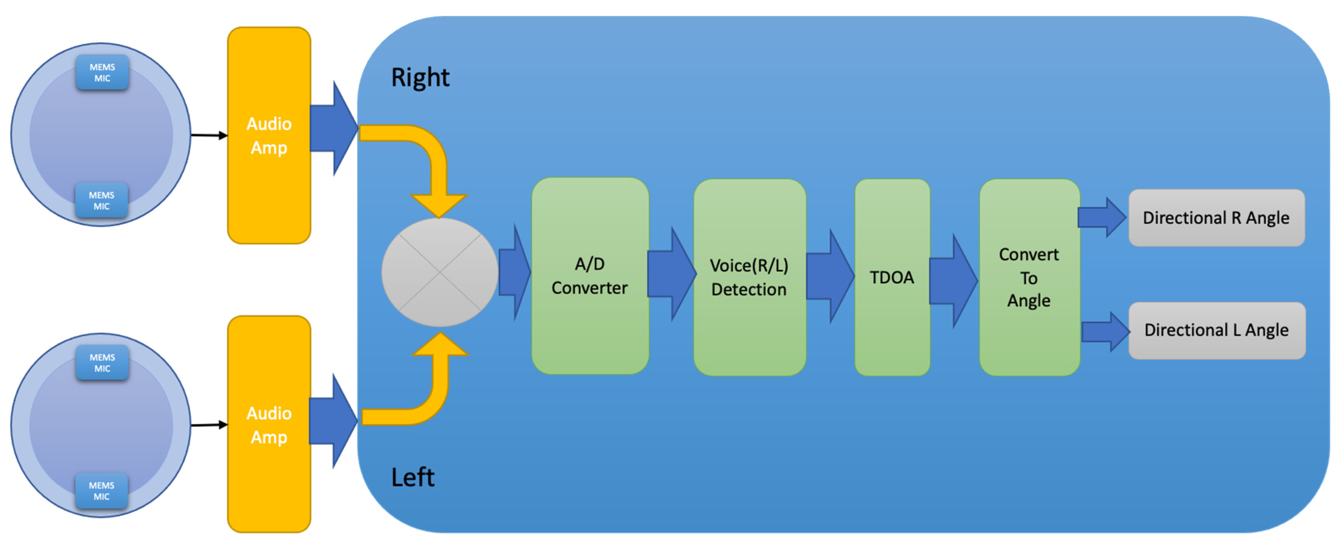
2.2. Signal Processing Method

Many algorithms have been proposed for acoustic localization for applications, including received signal strength indication (RSSI), time of arrival, time difference of arrival, and direction/angle of arrival [42,43,44]. For accuracy, some papers propose a mixture of two or three of the above positioning techniques, such as TOA-TDOA, TOA-AOA, TDOA-AOA, etc., whereas others detect and extract the relevant positioning parameters; then, they combine them with different algorithms to optimize final positioning performance.

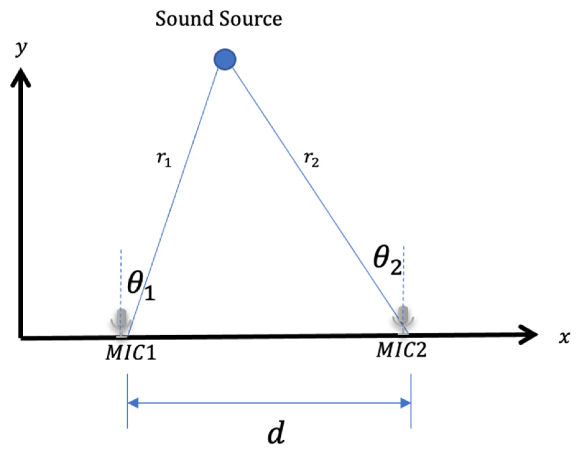
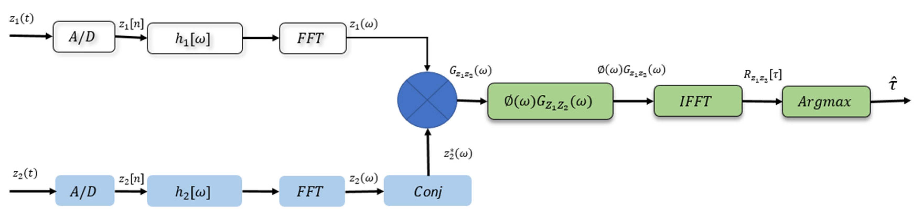
2.2.1. Time Difference of Arrival

Time difference of arrival is a popular technology used for distance measurement. This approach does not take the time to send the signal to the target but only the time to receive the signal and the signal propagation speed. The difference in arrival time can be used to measure the variation in distance from the target to the two reference points once the signal source is received at both reference points. Figure 3 illustrates a localization system implemented in TDOA using an acoustic source and two MIC Arrays.

Assume that there are multiple sound arrays in the detection area, defined as ${\mathrm{S}}_{\mathrm{m}}=\left\{{\mathrm{s}}_1\dots ,{\mathrm{s}}_{\mathrm{M}}\right\},\mathrm{m}\in \left\{1,2,\dots ,\mathrm{M}\right\}.$ Each ${\mathrm{s}}_{\mathrm{m}}$ can be specified as ${\mathrm{s}}_{\mathrm{m}}=\left({\mathrm{x}}_{\mathrm{m}},{\mathrm{y}}_{\mathrm{m}}\right)$.

Assume that the single target position state is ${\mathrm{p}}_{\mathrm{i}}=\left({\mathrm{px}}_{\mathrm{i}},{\mathrm{py}}_{\mathrm{i}}\right)$. Two acoustic sensors are used for each sensor group.

The time difference τ can be expressed as Equation (1):

$$\tau =\left|\frac{\Vert p_i-s_1\Vert -\Vert p_i-s_2\Vert }{v}\right|$$

(1)

where ${\mathrm{p}}_{\mathrm{i}}$ and ${\mathrm{s}}_{\mathrm{m}}$ are Cartesian coordinates. v is the sound velocity. ‖∙‖ is the Euclidean norm. For Sensor 1, the angle can be expressed as Equation (2).

$${\mathsf{\theta }}_1={\tan }^{-1}\left(\frac{p{x}_i-x_1}{p{y}_i-y_1}\right)$$

(2)

For Sensor 2, the angle can be expressed as Equation (3).

$${\mathsf{\theta }}_2={\tan }^{-1}\left(\frac{p{x}_i-x_2}{p{y}_i-y_2}\right)$$

(3)

2.2.2. Generalized Cross Correlation

GCC is based on finding the phase through the time difference, obtaining the correlation function with a steep peak value, finding the point when the correlation is maximum, and combining it with the sampling frequency to obtain direction information.

The left and right channels received by the microphone can be mathematically described as follows.

$$Z_1\left(t\right)={\alpha }_{1}s\left(t\right)+n_1\left(t\right)$$

(4)

$$Z_2\left(t\right)={\alpha }_{2}s\left(t-{\tau }_d\right)+n_2\left(t\right)$$

(5)

As illustrated in Figure 4, $Z_1\left(t\right)$ and $Z_2\left(t\right)$ represent the signals received from the left and right channels, respectively, $s\left(t\right)$ denotes the signal to be accepted for analysis, $n_1\left(t\right)$ and $n_2\left(t\right)$ represent the noise signals received in the air, respectively, ${\tau }_d$ is the time difference among the two sensors that detect the signal, and ${\alpha }_1$ and ${\alpha }_2$ are the magnitudes of the signal. The time difference can be obtained by the generalized correlation (GCC) method [45,46,47] for calculation.

$Z_{12}\left(\omega \right)$ is defined as the cross-power spectrum of signals $Z_1\left(t\right)$ and $Z_2\left(t\right)$ received by the two sensors.

$$Z_{12}\left(\omega \right)=Z_1\left(\omega \right)Z_2^{*}\left(\omega \right)$$

(6)

The cross-power spectral-density function is defined by the well-known Fourier transform relationship.

$$R_{Z_1{Z}_2}\left(\tau \right)={{\displaystyle \int }}_{-\infty }^{\infty }{Z}_{12}\left(\omega \right)e^{-j\omega \tau }d\omega$$

(7)

The GCC is denoted by $R_{Z_1{Z}_2}\left(\tau \right)$, the Fourier transform of $z_1\left(t\right)$ is denoted as $Z_1\left(\omega \right)$, and the Fourier transform of $Z_2^{*}\left(\omega \right)$ is a conjugate of $z_2\left(t\right)$. $\widehat{\tau }$ is defined as the arguments of the maxima $R_{Z_1{Z}_2}\left(\tau \right)$. ${\psi }_{1,2}\left(\omega \right)$ is defined as phase transform (PHAT), which was chosen as our weighting function to reduce ambient noise and reverberation interference. The equation is defined as ${\psi }_{1,2}\left(\omega \right)=\frac{1}{\left|G_{Z_1{Z}_2}\left(\omega \right)\right|}$.

GCC-PHAT can be estimated by the generalized cross-correlation (GCC) method and given.

$$R_{Z_1{Z}_2}\left(\tau \right)={{\displaystyle \int }}_{-\infty }^{\infty }{\psi }_{12}\left(\omega \right)Z_{12}\left(\omega \right)e^{-j\omega \tau }d\omega$$

(8)

$$\widehat{\tau }=arg max{R}_{Z_1{Z}_2}\left(\tau \right)$$

(9)

$${\psi }_{1,2}\left(\omega \right)=\frac{1}{\left|G_{Z_1{Z}_2}\left(\omega \right)\right|}=\frac{1}{\left|Z_{12}\left(\omega \right)\right|}$$

(10)

2.2.3. Sound Source Localization

This study of sound source localization is based on the use of generalized cross correlations and trigonometric functions to measure the location of a sound source. Instead of phase information, the arrival time difference of the signal between the elements is used. A generalized cross-correlation algorithm with a phase transformation is used to calculate arrival time difference. That is, the angle is calculated from the difference in arrival time.

The triangulation algorithm is based on the simple triangular function formula. As demonstrated in Figure 3, the MIC Array is assumed to be d apart, and the angle from the sound source to the two MIC arrays is ${\theta }_1$ and ${\theta }_2$. Equation (11) can be obtained.

$$d=y\tan {\theta }_1+y\tan {\theta }_2$$

(11)

Finally, we obtain the x and y of the sound source.

$$y=d/\left(\tan {\theta }_1+\tan {\theta }_2\right)$$

(12)

$$x=y\tan {\theta }_1$$

(13)

3. Results

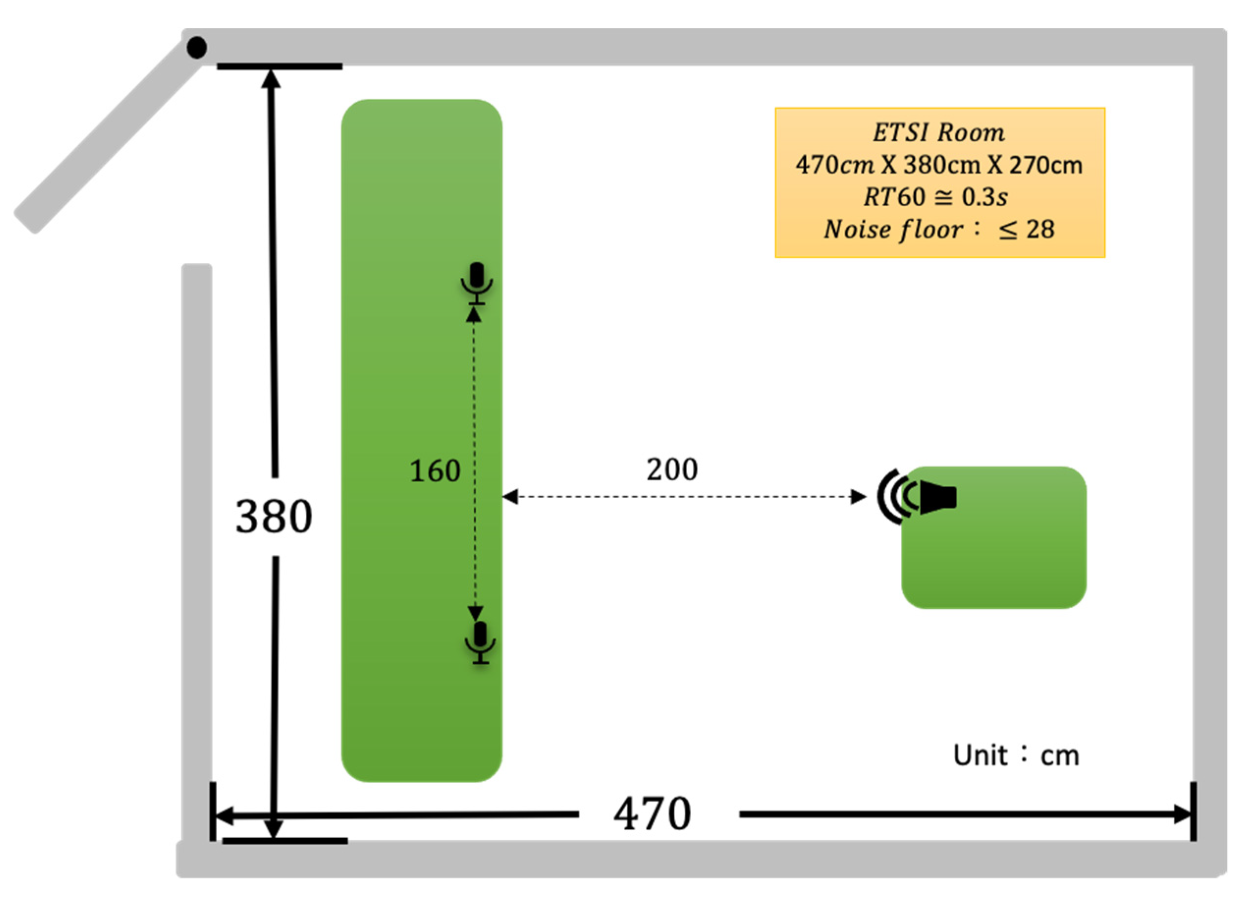
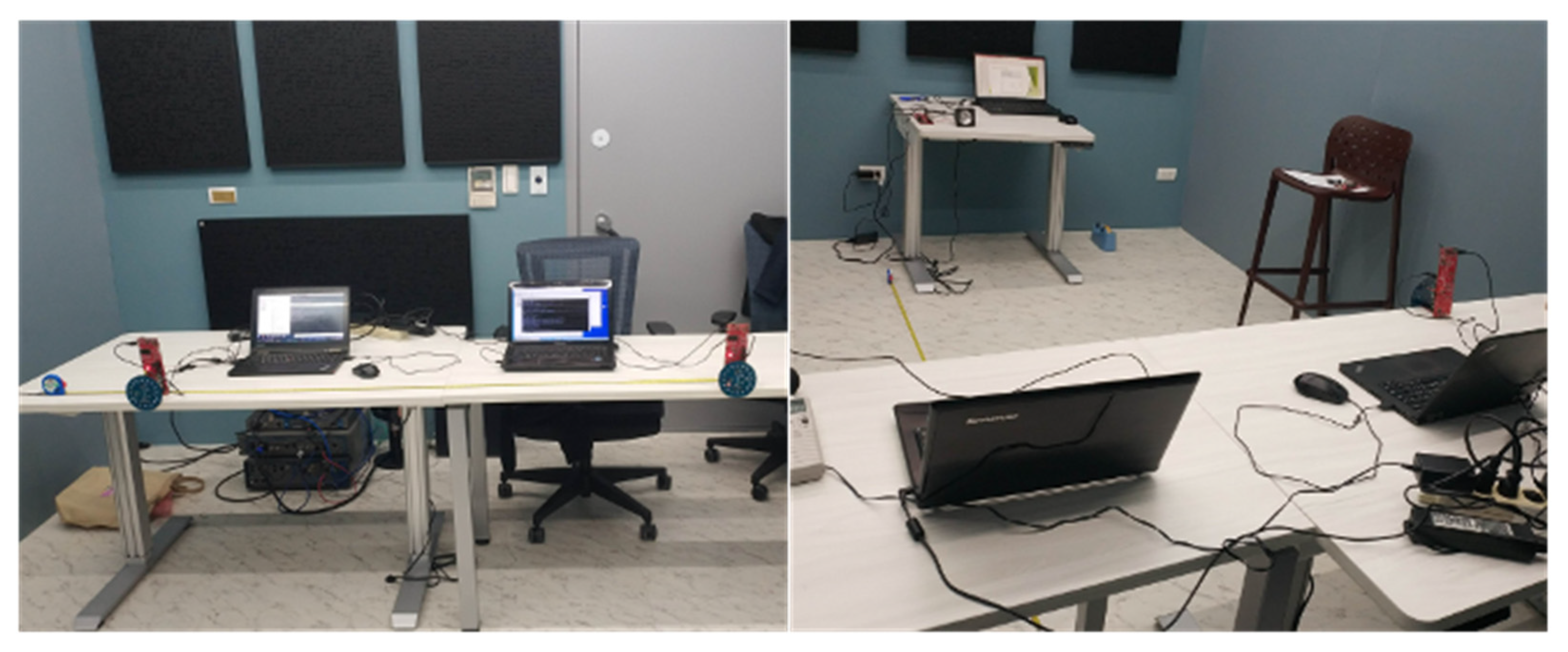
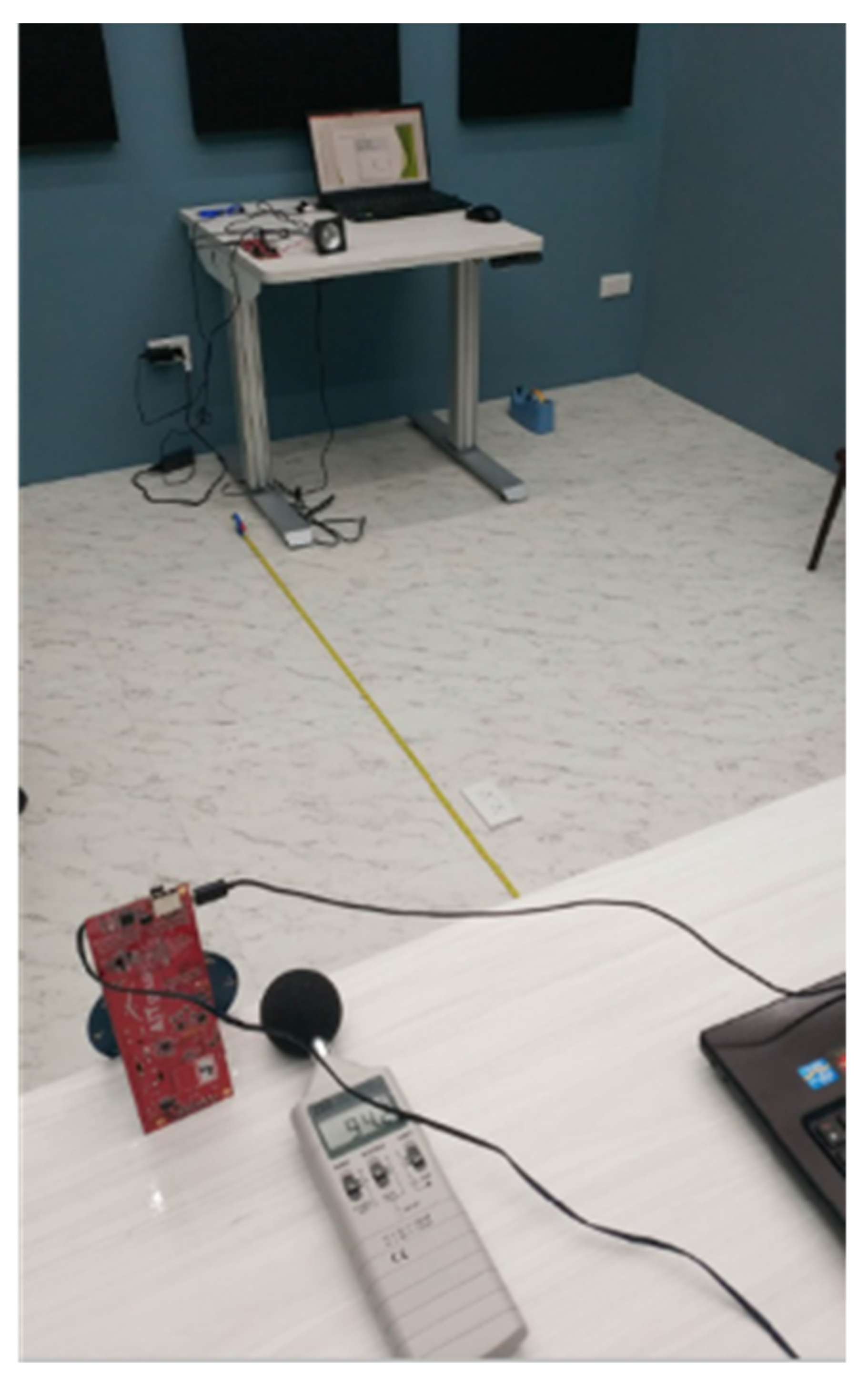
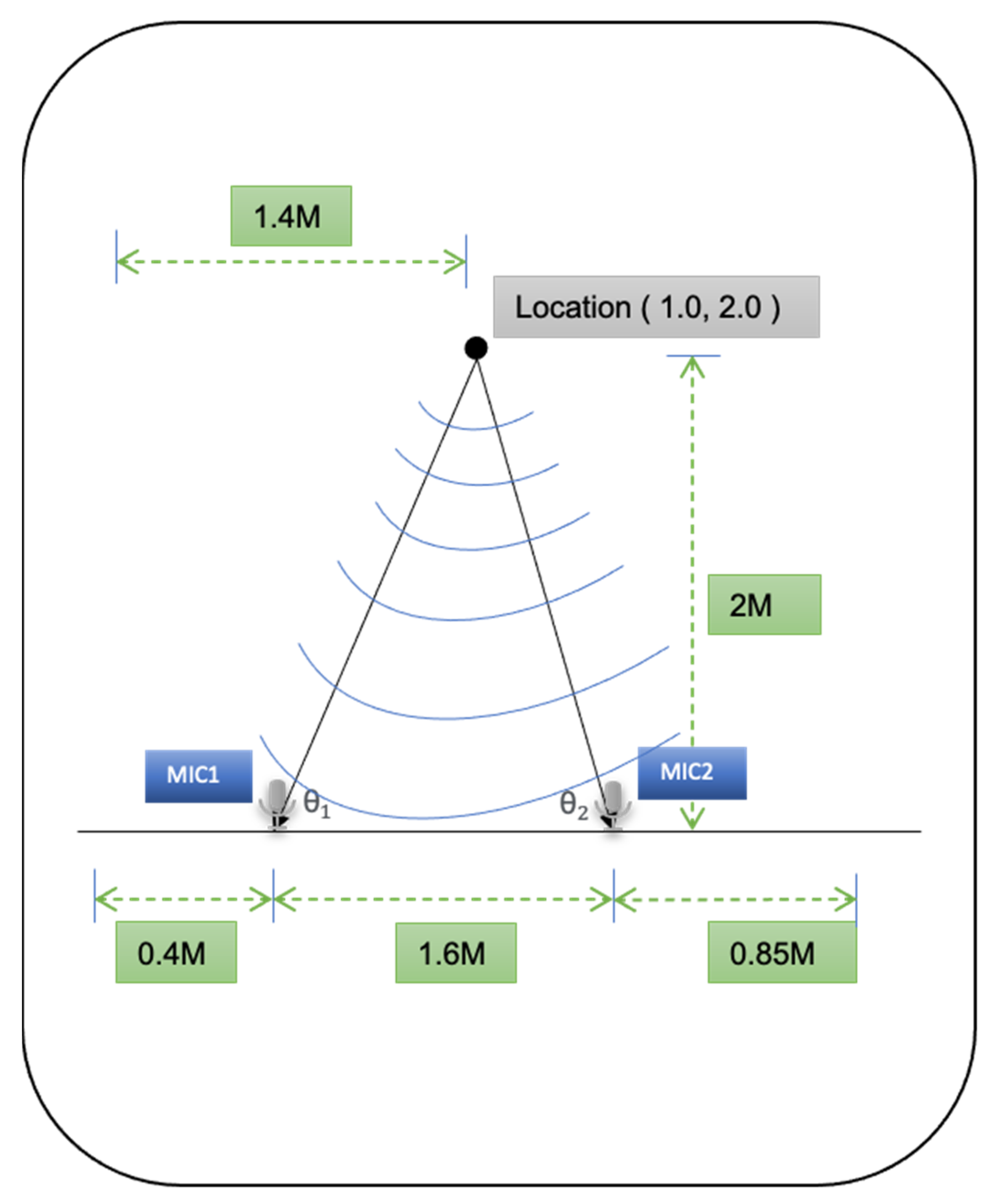
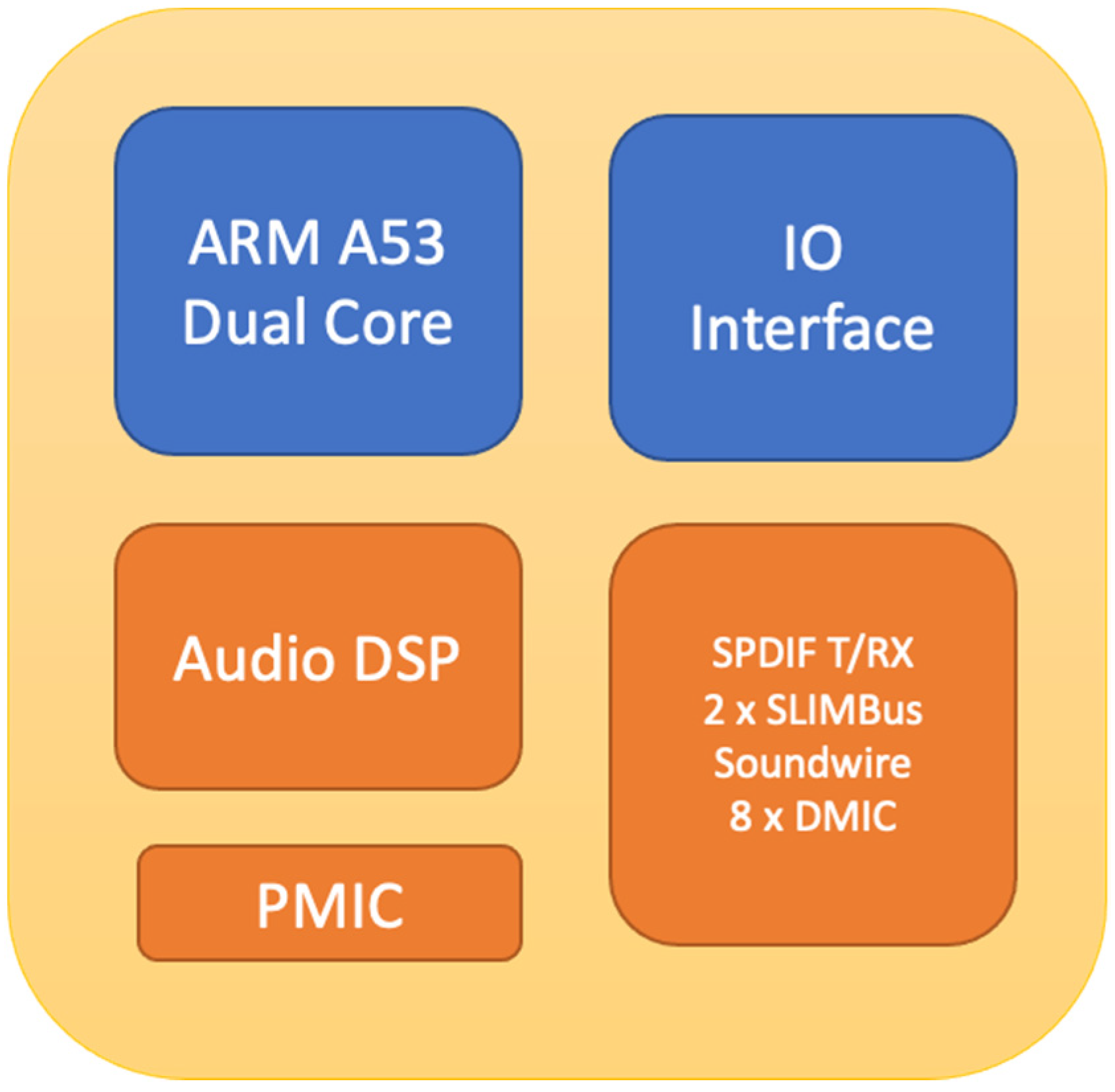
3.1. Testing Environment

In this study, the reverberation room with ETSI/T60 ≈ 0.3 S had a room size of 4.7 × 3.8 × 2.7 ${\mathrm{m}}^3$. The acoustic parameters of the listening room were measured by PAL Acoustics Technology Ltd. (Taipei, Taiwan) in May 2021. The laboratory has passed all European Telecommunications Standards Institute (ETSI) acoustic standard regulations. The test environment met the request of ISO7779-2018-11: Acoustics-Measurement of airborne noise emitted by information technology and telecommunications equipment. The environmental parameters of the laboratory were measured by the instruments of Brüel & Kjær. Brüel & Kjær is a professional equipment manufacturer for sound and vibration measurements. The laboratory will be calibrated once per year. Acoustic parameters are measured according to the following criteria:

• ISO 1996-1: Acoustics—Description, measurement and assessment of environmental noise-Part 1: Basic quantities and assessment procedures, 2003;
• ASTM Designation: E336-97 Standard Test Method for Measurement of Airborne Sound Insulation in Buildings;
• ASTM Designation: E413-16 Classification for Rating Sound Insulation.
• ISO 3382-2: 2008(E) Acoustics-Measurement of room acoustic parameters-Part 2: Reverberation time in ordinary rooms.

One microphone was placed on the left and right ends of the room in a straight line, and the sound source was placed in the middle of MIC1 and MIC2. The microphone was positioned at a vertical angle to the source, and the distance between the two microphones was 1.6 m. The distance between the source and the vertical angle of the microphone was 2 m. The top view of the ETSI room is illustrated by Figure 5 and Figure 6.

We will introduce the system model and analyze the key factors affecting positioning accuracy. To implement simple equipment, we considered a system with only one pair of microphones and one source.

With respect to objects with a single loudspeaker: The loudspeaker can be connected to the target object and play an acoustic signal. For the accuracy of the experiment, we added a decibel meter at the receiving end to make sure that the volume received by each test environment was consistent, as demonstrated in Figure 7. According to the specific application scenario, two microphones were used to receive the signal. To ensure the consistency of the received signal, the selected microphones must have the same characteristics; therefore, we selected the same brand of microphones to receive the audio source.

3.2. Experimental Methodology and Analysis of Results

3.2.1. Experiment 1: Measurement of Different Frequencies

As demonstrated in Figure 8, the signal to noise ratio (SNR) was fixed at 35. The speed of the sound wave propagation in air, measured by PAL Acoustic Technology Ltd. (Taipei, Taiwan) was 344 m/s. Angular accuracy was studied by analyzing the angular and (X, Y) errors presented by different frequencies from low to high in-context; the selected frequencies were 1 K, 5 K, 10 K, 12 K, and 15 K. The position coordinates of the measurement target were (1.4, 2.0). We predicted that the errors would increase as frequency increased. The distance between the X-axis and the Y-axis was significantly different from the actual distance at lower frequencies. The angular error was also larger at lower frequencies. The estimation error at the same speed decreased as frequency increased. From the analysis results, we can observe that the error value became more stable at about 10 K.

Table 2. Frequency and angular error table.

Frequency/Hz	Angular Error
	${\mathit{\theta }}_1$	${\mathit{\theta }}_2$	Average
1 k	10.641	7.861	9.25
2 k	2.0878	9.777	5.93
3 k	0.3012	3.3485	1.82
4 k	3.1258	3.0462	3.09
5 k	2.5395	1.1583	1.85
6 k	0.2682	2.0954	1.18
7 k	1.1033	0.2188	0.66
8 k	1.3596	0.3753	0.87
9 k	1.153	0.5023	0.83
10 k	0.988	0.4831	0.74
11 k	0.7901	0.8688	0.83
12 k	0.2022	1.2288	0.72
13 k	1.1424	0.0251	0.58
14 k	0.5973	0.0048	0.30
15 k	0.009	1.1542	0.58

and

Table 3. Comparison of frequency and distance offsets.

Frequency/Hz	Distance Offset(cm)
	X	Y	Max
1 k	−41.01	−2.43	41.01
2 k	28.55	−16.26	28.55
3 k	−8.10	15.36	15.36
4 k	−5.65	−37.81	37.81
5 k	1.63	16.22	16.22
6 k	1.00	2.1449	2.14
7 k	1.00	1.9464	1.95
8 k	1.45	3.42	3.42
9 k	−2.26	−5.11	5.11
10 k	0.99	1.9098	1.91
11 k	0.93	−1.94	1.94
12 k	−3.09	1.72	3.09
13 k	0.98	2.0033	2.00
14 k	1.01	1.9815	1.98
15 k	−0.48	−7.44	7.44

analyze the error limits of the angle and X and Y coordinates. The higher the frequency, the more stable the angle and (X, Y), and the higher the accuracy, as demonstrated in Table 3. Considering the characteristics of most microphones and speakers on the market, we chose 10 K as our reference frequency.

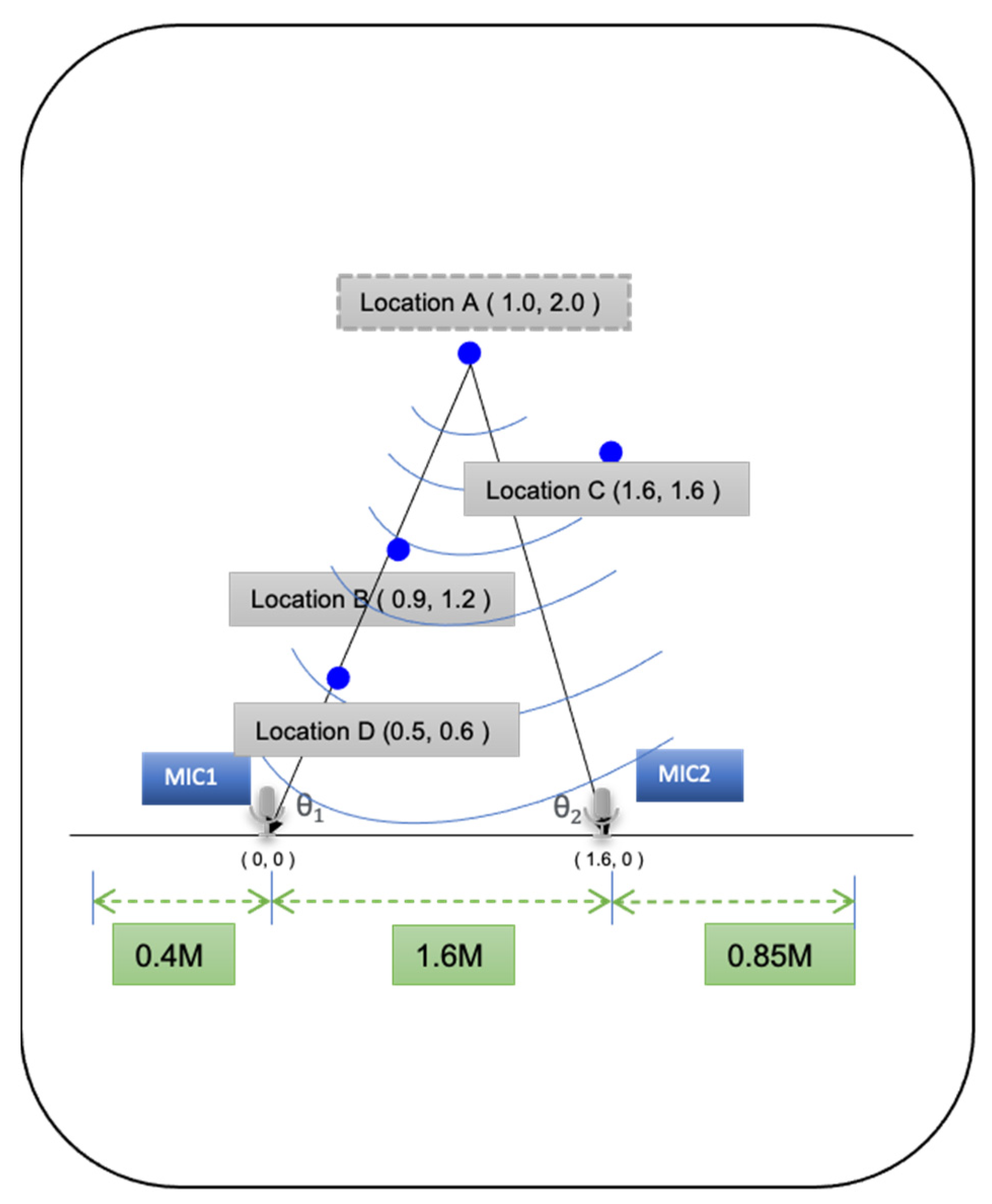
3.2.2. Experiment 2: Sound Source Estimation Position Accuracy Test

To verify the frequencies proposed in Experiment 1, four different locations were used, namely Location A (1.0, 2.0), Location B (0.9, 1.2), Location C (1.6, 1.6), and Location D (0.5, 0.6), as illustrated in Figure 9. To consider sound propagation in the air at 344 m/s for whether the microphone is far away or close to the different angles and whether there is a difference due to the different locations, the results of the experiment demonstrate that the measured original location and the three newly created different locations’ accuracies are similar, as portrayed in

Table 4. Accuracy in different positions.

	Target (X, Y) (m)	Measure (X, Y) (m)	Accuracy (X, Y) (cm)
Location A	(1.0, 2.0)	(0.98, 2.02)	(2.32, 2.02)
Location B	(0.9, 1.2)	(0.91, 1.22)	(1.30, 1.55)
Location C	(1.6, 1.6)	(1.59, 1.58)	(−0.40, −1.9)
Location D	(0.5, 0.6)	(0.49, 0.58)	(−0.41, −1.55)

.

3.3. Discussion

The compressive theory [38] of the microphone array sound source localization method has better noise immunity compared to the traditional localization method. Most methods of sound source localization are implemented in two steps with compressive technology. First, the direction of arrival (DOA) or TDOA from the different microphones of the received signals is estimated; then, the source location is estimated. Compressive technology collects audio data at a rate much lower than the Nyquist rate. This improves localization accuracy and enables direct source localization, which does not require DOA or TDOA estimations. However, for accuracy, ref. [38] proposed a microphone array source localization method based on CS theory. The space is divided into a grid structure, but it can be observed from the results that a higher number of microphones result in a smaller error value. As the amount of microphones increases, localization capabilities become better, but this constitutes an increase in cost. In [39], the IMGD calculation method is proposed to investigate how the architecture in MGD can be used with other algorithms to increase accuracy. The MUSIC group delay (MGD) method is applicable to near-range signals. However, it is computationally costly and requires large arrays. To solve these limitations, ref. 39] proposed an improved MGD (IMGD) method. Although the authors improved efficiency, MGD requires additional complex algorithms to perform more complicated calculations. Moreover, it increases system usage when performing this operation. Therefore, the use of compressive microphones or other algorithms increases the complexity or cost of the system. In this study, we used known operating frequencies with simple GCC without additional algorithms. The best operating frequency was located according to the frequency point regarding angle and distance error, respectively. From 1 K to 15 K, the best operating frequency was explored at each frequency point. The results are displayed in Table 2 for the angular error and Table 3 for the distance error. Accuracy can be achieved at the frequency point of 10 K, as demonstrated in

Table 5. Accuracy compared to the literature.

Method	Accuracy		Number of Microphones
	Position(cm)	Angle
[38]	19.75	-	12
[39]	-	2°	8
Proposed	2.02~2.3	0.74°	4

.

4. Conclusions

Sound source localization has been used in many applications, and previous experiments have included many techniques, such as TDOA, AOA, and DOA [28]. This study used TDOA in combination with the GCC algorithm to improve TDOA calculation results by working with real acoustic signals at optimal frequencies. The GCC technique attempts to find the most stable operating frequency between different frequencies and achieve a certain accuracy level with a minimum number of microphones. We conducted experiments and proved that this method is effective in practice. This is a stable and straightforward method for locating sound sources. In this study, we only focused on the localization of a single sound source. In future research work, we can focus on how to localize moving sound sources under this framework, i.e., how to localize them accurately considering the Doppler effect.

References

1. Barbieri, L.; Brambilla, M.; Trabattoni, A.; Mervic, S.; Nicoli, M. UWB localization in a smart factory: Augmentation methods and experimental assessment. IEEE Trans. Instrum. Meas. 2021, 70, 1–18. [Google Scholar] [CrossRef]
2. Shi, D.; Mi, H.; Collins, E.G.; Wu, J. An indoor low-cost and high-accuracy localization approach for AGVs. IEEE Access 2020, 8, 50085–50090. [Google Scholar] [CrossRef]
3. Yi, D.-H.; Lee, T.-J.; Cho, D.-I. A new localization system for indoor service robots in low luminance and slippery indoor environment using afocal optical flow sensor based sensor fusion. Sensors 2018, 18, 171. [Google Scholar] [CrossRef] [PubMed] [Green Version]
4. Li, B.; Lu, Y.; Karimi, H.R. Adaptive Fading Extended Kalman Filtering for Mobile Robot Localization Using a Doppler–Azimuth Radar. Electronics 2021, 10, 2544. [Google Scholar] [CrossRef]
5. Upadhyay, J.; Rawat, A.; Deb, D.; Muresan, V.; Unguresan, M.-L. An RSSI-based localization, path planning and computer vision-based decision making robotic system. Electronics 2020, 9, 1326. [Google Scholar] [CrossRef]
6. Ryumin, D.; Kagirov, I.; Axyonov, A.; Pavlyuk, N.; Saveliev, A.; Kipyatkova, I.; Zelezny, M.; Mporas, I.; Karpov, A. A multimodal user interface for an assistive robotic shopping cart. Electronics 2020, 9, 2093. [Google Scholar] [CrossRef]
7. Savkin, A.V.; Huang, H. Range-based reactive deployment of autonomous drones for optimal coverage in disaster areas. IEEE Trans. Syst. Man Cybern. Syst. 2021, 51, 4606–4610. [Google Scholar] [CrossRef]
8. Muhammad, K.; Ahmad, J.; Lv, Z.; Bellavista, P.; Yang, P.; Baik, S.W. Efficient deep CNN-based fire detection and localization in video surveillance applications. IEEE Trans. Syst. Man Cybern. Syst. 2018, 49, 1419–1434. [Google Scholar] [CrossRef]
9. Shah, S.A.; Fioranelli, F. RF sensing technologies for assisted daily living in healthcare: A comprehensive review. IEEE Aerosp. Electron. Syst. Mag. 2019, 34, 26–44. [Google Scholar] [CrossRef] [Green Version]
10. Kim, S.-C.; Jeong, Y.-S.; Park, S.-O. RFID-based indoor location tracking to ensure the safety of the elderly in smart home environments. Pers. Ubiquitous Comput. 2013, 17, 1699–1707. [Google Scholar] [CrossRef]
11. Zhou, M.; Wang, Y.; Liu, Y.; Tian, Z. An information-theoretic view of WLAN localization error bound in GPS-denied environment. IEEE Trans. Veh. Technol. 2019, 68, 4089–4093. [Google Scholar] [CrossRef]
12. Becerra, V.M. Autonomous control of unmanned aerial vehicles. Electronics 2019, 8, 452. [Google Scholar] [CrossRef] [Green Version]
13. Al-Sadoon, M.A.G.; De Ree, M.; Abd-Alhameed, R.A.; Excell, P.S. Uniform sampling methodology to construct projection matrices for Angle-of-Arrival estimation applications. Electronics 2019, 8, 1386. [Google Scholar] [CrossRef] [Green Version]
14. Luo, M.; Chen, X.; Cao, S.; Zhang, X. Two new shrinking-circle methods for source localization based on TDoA measurements. Sensors 2018, 18, 1274. [Google Scholar] [CrossRef] [PubMed] [Green Version]
15. Xu, C.; Ji, M.; Qi, Y.; Zhou, X. MCC-CKF: A distance constrained Kalman filter method for indoor TOA localization applications. Electronics 2019, 8, 478. [Google Scholar] [CrossRef] [Green Version]
16. Vera-Diaz, J.M.; Pizarro, D.; Macias-Guarasa, J. Towards end-to-end acoustic localization using deep learning: From audio signals to source position coordinates. Sensors 2018, 18, 3418. [Google Scholar] [CrossRef] [PubMed] [Green Version]
17. Fabregat, G.; Belloch, J.A.; Badia, J.M.; Cobos, M. Design and implementation of acoustic source localization on a low-cost IoT edge platform. IEEE Trans. Circuits Syst. II Express Briefs 2020, 67, 3547–3551. [Google Scholar] [CrossRef]
18. Salvati, D.; Drioli, C.; Foresti, G.L. A low-complexity robust beamforming using diagonal unloading for acoustic source localization. IEEE/ACM Trans. Audio Speech Lang. Processing 2018, 26, 609–622. [Google Scholar] [CrossRef] [Green Version]
19. Xue, C.; Zhong, X.; Cai, M.; Chen, H.; Wang, W. Audio-Visual Event Localization by Learning Spatial and Semantic Co-attention. IEEE Trans. Multimed. 2021. [Google Scholar] [CrossRef]
20. Arakawa, T. Recent research and developing trends of wearable sensors for detecting blood pressure. Sensors 2018, 18, 2772. [Google Scholar] [CrossRef] [PubMed] [Green Version]
21. Chien, J.-C.; Dang, Z.-Y.; Lee, J.-D. Navigating a service robot for indoor complex environments. Appl. Sci. 2019, 9, 491. [Google Scholar] [CrossRef] [Green Version]
22. Han, J.-H. Tracking control of moving sound source using fuzzy-gain scheduling of PD control. Electronics 2020, 9, 14. [Google Scholar] [CrossRef] [Green Version]
23. Yvanoff-Frenchin, C.; Ramos, V.; Belabed, T.; Valderrama, C. Edge Computing Robot Interface for Automatic Elderly Mental Health Care Based on Voice. Electronics 2020, 9, 419. [Google Scholar] [CrossRef] [Green Version]
24. Liang, M.; Xi-Hai, L.; Wan-Gang, Z.; Dai-Zhi, L. The generalized cross-correlation Method for time delay estimation of infrasound signal. In Proceedings of the 2015 Fifth International Conference on Instrumentation and Measurement, Computer, Communication and Control (IMCCC), Qinhuangdao, China, 18–20 September 2015; pp. 1320–1323. [Google Scholar]
25. Hożyń, S. A Review of Underwater Mine Detection and Classification in Sonar Imagery. Electronics 2021, 10, 2943. [Google Scholar] [CrossRef]
26. Shi, F.; Chen, Z.; Cheng, X. Behavior modeling and individual recognition of sonar transmitter for secure communication in UASNs. IEEE Access 2019, 8, 2447–2454. [Google Scholar] [CrossRef]
27. Lemieszewski, Ł.; Radomska-Zalas, A.; Perec, A.; Dobryakova, L.; Ochin, E. The Spoofing Detection of Dynamic Underwater Positioning Systems (DUPS) Based on Vehicles Retrofitted with Acoustic Speakers. Electronics 2021, 10, 2089. [Google Scholar] [CrossRef]
28. Sakavičius, S.; Serackis, A. Estimation of Azimuth and Elevation for Multiple Acoustic Sources Using Tetrahedral Microphone Arrays and Convolutional Neural Networks. Electronics 2021, 10, 2585. [Google Scholar] [CrossRef]
29. Seo, S.-W.; Yun, S.; Kim, M.-G.; Sung, M.; Kim, Y. Screen-based sports simulation using acoustic source localization. Appl. Sci. 2019, 9, 2970. [Google Scholar] [CrossRef] [Green Version]
30. Pu, H.; Cai, C.; Hu, M.; Deng, T.; Zheng, R.; Luo, J. Towards robust multiple blind source localization using source separation and beamforming. Sensors 2021, 21, 532. [Google Scholar] [CrossRef] [PubMed]
31. Huang, G.; Benesty, J.; Cohen, I.; Chen, J. A simple theory and new method of differential beamforming with uniform linear microphone arrays. IEEE/ACM Trans. Audio, Speech Lang. Process. 2020, 28, 1079–1093. [Google Scholar] [CrossRef]
32. Piotto, M.; Ria, A.; Stanzial, D.; Bruschi, P. Design and characterization of acoustic particle velocity sensors fabricated with a commercial post-CMOS MEMS process. In Proceedings of the 2019 20th International Conference on Solid-State Sensors, Actuators and Microsystems & Eurosensors XXXIII (TRANSDUCERS & EUROSENSORS XXXIII), Berlin, Germany, 23–27 June 2019; pp. 1839–1842. [Google Scholar]
33. Wang, Z.Q.; Le Roux, J.; Hershey, J.R. Multi-channel deep clustering: Discriminative spectral and spatial embeddings for speaker-independent speech separation. In Proceedings of the 2018 IEEE International Conference on Acoustics, Speech and Signal Processing (ICASSP), Calgary, AB, Canada, 15–20 April 2018; pp. 1–5. [Google Scholar]
34. Liu, L.; Li, Y.; Kuo, S.M. Feed-forward active noise control system using microphone array. IEEE/CAA J. Autom. Sin. 2018, 5, 946–952. [Google Scholar] [CrossRef]
35. Qin, M.; Hu, D.; Chen, Z.; Yin, F. Compressive Sensing-Based Sound Source Localization for Microphone Arrays. Circuits, Syst. Signal Process. 2021, 40, 4696–4719. [Google Scholar] [CrossRef]
36. VandenDriessche, J.; Da Silva, B.; Lhoest, L.; Braeken, A.; Touhafi, A. M3-AC: A Multi-Mode Multithread SoC FPGA Based Acoustic Camera. Electronics 2021, 10, 317. [Google Scholar] [CrossRef]
37. Singh, A.P.; Tiwari, N. An improved method to localize simultaneously close and coherent sources based on symmetric-Toeplitz covariance matrix. Appl. Acoust. 2021, 182, 108176. [Google Scholar] [CrossRef]
38. Kim, S.; Park, M.; Lee, S.; Kim, J. Smart Home Forensics—Data Analysis of IoT Devices. Electronics 2020, 9, 1215. [Google Scholar] [CrossRef]
39. Isyanto, H.; Arifin, A.S.; Suryanegara, M. Design and implementation of IoT-based smart home voice commands for disabled people using Google Assistant. In Proceedings of the 2020 International Conference on Smart Technology and Applications (ICoSTA), Surabaya, Indonesia, 20–20 February 2020; pp. 1–6. [Google Scholar]
40. Chan-Ley, M.; Olague, G.; Altamirano-Gomez, G.E.; Clemente, E. Self-localization of an uncalibrated camera through invariant properties and coded target location. Appl. Opt. 2020, 59, D239–D245. [Google Scholar] [CrossRef] [PubMed]
41. Krause, M.; Müller, M.; Weiß, C. Singing Voice Detection in Opera Recordings: A Case Study on Robustness and Generalization. Electronics 2021, 10, 1214. [Google Scholar] [CrossRef]
42. Li, X.; Xing, Y.; Zhang, Z. A Hybrid AOA and TDOA-Based Localization Method Using Only Two Stations. Int. J. Antennas Propag. 2021, 2021, 1–8. [Google Scholar] [CrossRef]
43. Kraljevic, L.; Russo, M.; Stella, M.; Sikora, M. Free-Field TDOA-AOA Sound Source Localization Using Three Soundfield Microphones. IEEE Access 2020, 8, 87749–87761. [Google Scholar] [CrossRef]
44. Khalaf-Allah, M. Particle filtering for three-dimensional TDoA-based positioning using four anchor nodes. Sensors 2020, 20, 4516. [Google Scholar] [CrossRef]
45. Tian, Z.; Liu, W.; Ru, X. Multi-Target Localization and Tracking Using TDOA and AOA Measurements Based on Gibbs-GLMB Filtering. Sensors 2019, 19, 5437. [Google Scholar] [CrossRef] [Green Version]
46. Carter, G. Coherence and time delay estimation. Proc. IEEE 1987, 75, 236–255. [Google Scholar] [CrossRef]
47. Knapp, C.; Carter, G. The generalized correlation method for estimation of time delay. IEEE Trans. Acoust. Speech Signal Process. 1976, 24, 320–327. [Google Scholar] [CrossRef] [Green Version]
Figure 1. Sound source estimation system blocks.
Electronics 11 00890 g001
Figure 2. Processor architecture for the microphone array.
Electronics 11 00890 g002
Figure 3. A pair of sensor array model diagrams.
Electronics 11 00890 g003
Figure 4. Generalized cross correlation-PHAT block diagram.
Electronics 11 00890 g004
Figure 5. ETSI Chamber environment map.
Electronics 11 00890 g005
Figure 6. ETSI Chamber actual test setup.
Electronics 11 00890 g006
Figure 7. Sound source volume calibration chart.
Electronics 11 00890 g007
Figure 8. Sound source volume calibration chart.
Electronics 11 00890 g008
Figure 9. Location of the 4 test points.
Electronics 11 00890 g009