Coverage Optimization of Wireless Sensor Networks Using Combinations of PSO and Chaos Optimization

Abstract

The coverage rate is the most crucial index in wireless sensor networks (WSNs) design; it involves making the sensors with a reasonable distribution, which closely relates to the quality of service (QoS) and survival period of the entire network. This article proposes to use particle swarm optimization (PSO) and chaos optimization in conjunction for the coverage optimization. All sensor locations are encoded together as a particle position. PSO was used first to make sensors move close to their optimal positions; furthermore, a variable domain chaos optimization algorithm (VDCOA) was employed to reach a higher coverage rate, along with improved evenness and average moving distance. Six versions of VDCOA, taking circle, logistic, Gaussian, Chebyshev, sinusoidal and cubic maps, respectively, were investigated. The simulation experiment tested three cases: square, rectangular and circular regions using nine algorithms: six versions of PSO plus VDCOA, PSO and other two PSO variants. All six versions showed better performance than PSO and CPSO, with coverage all exceeding 90% for the first two cases. Moreover, one version, PSO plus circle map (PSO-Circle), increased the coverage rate by 3.17%, 2.41% and 12.94% compared with PSO in three cases, respectively, and outperformed the other eight algorithms.

1. Introduction

Over the last decades, wireless sensor networks (WSNs) technology has made great progress; its application has involved industry, agriculture, environment protection, medical service and many other fields [1,2,3]. With the rise of the internet of things and the coming of the big data era, wireless sensor networks will face increasing requirements and rapid development [4]. Coverage rate is the crucial index to evaluate the performance of WSN; well-designed wireless sensor networks should have a high coverage, which decreases the blind area and increases the sensitiveness of the network perception [5]. The high coverage is also helpful to improve the energy efficiency and to enhance the endurance of all the sensor nodes [6]. Therefore, the coverage study of WSNs has attracted much interest, and many research results have been issued in recent years. Jia et al. discussed the multi-objective coverage algorithm for WSNs [7]. Guo et al. [8] proposed to use a quantum-inspired cultural algorithm for the multi-objective optimization of WSNs, considering both energy-saving and coverage rate indexes. Whale optimization algorithm (WOA), inspired by the whales’ rounding for prey, is also used in WSNs optimization. Wang et al. [9] introduced reverse learning into WOA to improve the coverage of WSNs. Deepa et al. [10] proposed to use levy flight to enhance WOA for guaranteeing the network coverage. Other intelligent optimization algorithms, including the bee algorithm [11,12], the weed algorithm [13], the wolf pack algorithm [14], the glowworm swarm optimization [15,16], the social spider optimization (SSO) algorithm [17], the multi-objective immune co-evolutionary algorithm (MOICEA) [18], the simulated annealing (SA) [19], the ant colony optimization (ACO) [20], the combined optimization using chaotic flower pollination and cuckoo algorithms [21], the biogeography-based optimization [22], the grey wolf optimizer [23,24] and the termite flies optimization (TFO) algorithm [25]. Other works also include linear programming optimization [26], the barrier coverage algorithm [27], and the coverage and connectivity problem solving of large sensor networks [28]. Tarnaris et al. [29] evaluated the performance of particle swarm and genetic algorithms in solving WSNs coverage problems via comparative simulation tests.

Particle swarm optimization (PSO), developed in the last two decades [30], has some distinct advantages, such as simpler iteration rules and higher convergence speed compared with other intelligent optimization methods. The PSO method has gained successful applications in many engineering fields. Wang et al. [31] discussed the dynamic deployment optimization of WSNs with co-evolutionary PSO algorithms. Sun et al. [32] presented an improved global PSO algorithm by hybridizing shuffled frog leaping optimization. Wang et al. put forward a coverage algorithm based on a PSO algorithm and combinatorial mathematics [33]. Zhang et al. [34] introduced an immune method into a PSO algorithm to optimize the K-barrier coverage. Bai et al. [35] increased the k-coverage of WSNs through an improved PSO algorithm under limited mobility. Xu et al. [36] integrated a discrete particle swarm algorithm into a new hybrid-MOEA/D-II algorithm for WSNs coverage optimization. Wang et al. [37] combined a PSO algorithm with simulated annealing for WSNs energy-efficient coverage.

To sum up the above, using heuristic algorithms to optimize WSNs coverage is a hot topic, especially the popular and effective PSO algorithm. When these heuristic algorithms, including the PSO algorithm, are used in WSNs, there are two prime ways: one is to improve the algorithm itself, the other is to combine another algorithm to form a hybrid algorithm to strengthen the performance in solving WSNs coverage.

Chaos is taken as an optimization method for the chaotic map can create a non-repetitive sequence instead of random sequence. Chaos optimization is usually employed as an auxiliary means of other algorithms. It is often used as the local search method to add perturbation in order to avoid premature convergence or is taken to optimize the parameters of the other algorithm when combined with other algorithms.

In this article, PSO and chaos optimization are proposed to improve the coverage rate for solution of the WSNs sensors deployment. This new proposed approach combines the advantages of PSO and chaos optimization; meanwhile, to improve the general chaos optimization, this article put forward a variable domain chaos optimization algorithm (VDCOA). The VDCOA adds adaptive adjustment on the center and boundary of the chaotic searching on the basis of common chaos optimization. Specifically, VDCOA employs multiple one-dimensional chaotic maps to search; as the iteration continues, the boundary of the search domain is linearly decreased. Moreover, once a better point is found by any chaos map, the center is updated by this new better point and another new round chaotic mapping is restarted. The VDCOA is a new chaos optimization method and is different from any existing chaos algorithm. In addition, this article investigates the six versions of VDCOA, in which the employed chaotic maps are circle map, logistic map, Gaussian map, Chebyshev map, sinusoidal map and cubic map, respectively. For simplicity of description, the combination of PSO with VDCOA is called PSO-VDCOA, and its six specific versions are called PSO-Circle, PSO-Logistic, PSO-Gaussian, PSO-Chebyshev, PSO-Sinusoidal and PSO-Cubic, respectively. To realize the optimal coverage of the WSNs, this article first discusses the network model, establishes the coverage rate optimization model, and further presents six chaos maps and the proposed PSO-VDCOA and its detailed procedures for the coverage optimization. Finally, numerical experiments, including the comparison of the six versions of PSO-VDCOA with three other PSO algorithms, are carried out to test the algorithm.

The remainders of this article are organized as follows. The detailed coverage model of WSNs is established in Section 2. In the next section, the algorithm combination of the particle swarm optimization algorithm and the chaos optimization algorithm (namely, PSO-VDCOA) are put forward for WSNs coverage optimization. In Section 4, the simulation experiment verification of PSO-VDCOA is completed. In the end, some conclusions will be presented in Section 5.

2. Model of Wireless Sensor Networks

It is supposed that m sensors will be assigned in the monitoring region, and that all the sensor nodes form a set as S = {n₁, n₂, …, n_i, …, n_m−1, n_m}, where n_i denotes the ith node with its coordinate as (x_i, y_i). For any point p with its coordinate (x_p, y_p) in the monitoring region, using the probability model in the literature [13], the probability of node n_i detecting the target point t can be modeled as

$$P_t(n_i,t)=\{\begin{array}{cc}1& d(n_i,t)\le r_s-r_e\\ \exp \left(\frac{-{\lambda }_1{\alpha }_1^{{\beta }_1}}{{\alpha }_2^{{\beta }_2}+{\lambda }_2}\right)& r_s-r_e<d(n_i,t)<r_s+r_e\\ 0& other cases\end{array},$$

(1)

where $d(n_i,t)$ is the Euclidean distance from node n_i to the target point t, $r_s$ is the sensing range and $r_e$ is the sensing reliability parameter of the single sensor node, $0<r_e<r_s$, ${\alpha }_1=r_e-r_s+d(n_i,t)$, ${\alpha }_2=r_e+r_s-d(n_i,t)$, ${\lambda }_1$, ${\lambda }_2$, ${\beta }_1$ and ${\beta }_2$ are all sensing coefficients related to node characteristics.

The combined probability of all the sensor nodes in the entire monitoring region to detect the target point t is

$$P_t(n_{all},t)=1-{\displaystyle \prod _{i=1}^m(1-P_t(n_i,t))},$$

(2)

where n_all is the set of all the sensors that can detect the target point t.

To compute the coverage rate for the entire network, the monitoring region is divided into l × n grids; each grid is in the shape of a rectangle section, and each section has an equal region of 1 m × 1 m and is simplified as a pixel with discretized precision of 1 m². Thus, the coverage rate of the wireless sensor network is defined as the ratio of the detectable grid point number to the total grid point number:

$$C=\frac{{\displaystyle \sum _{x_t=1}^l{\displaystyle \sum _{y_t=1}^n{P}_t(n_{all},t)}}}{l\times n},$$

(3)

Evenness is also an index to evaluate the performance of wireless sensor networks. Higher evenness means the more uniform nodes distribution, which ensures the lower energy consumption and the longer survival period. The evenness of single node n_i is computed as

$$U_i=\sqrt{\frac{1}{k_i}{\displaystyle \sum _{j=1}^{k_i}{\left(D_{i,j}-M_i\right)}^2}},$$

(4)

where $k_i$ is the neighbor nodes number, $D_{i,j}$ is the distance from node n_i to node n_j, $M_i$ is the mean value of all the distances from node n_i to all its neighbor nodes.

The evenness of the entire wireless sensor network is

$$U=\frac{1}{m}{\displaystyle \sum _{i=1}^m{U}_i}=\frac{1}{m}{\displaystyle \sum _{i=1}^m\sqrt{\frac{1}{k_i}{\displaystyle \sum _{j=1}^{k_i}{\left(D_{i,j}-M_i\right)}^2}}},$$

(5)

where m is the total nodes number.

According to the definition of Equation (5), lower U value means higher evenness. Besides, the average moving distance is also used to evaluate the total energy consumption from all nodes moving, and is defined as

$$D_m=\frac{1}{m}{\displaystyle \sum _{i=1}^m\sqrt{{\left(x_i-x_0\right)}^2+{\left(y_i-y_0\right)}^2}}$$

(6)

where $x_0$, $y_0$ are the initial coordinates of node n_i before coverage optimization, and $x_i$, $y_i$ are the new values of node n_i after coverage optimization.

3. Combined Using of PSO and VDCOA for WSNs Coverage Optimization

3.1. Overview of Particle Swarm Optimization

The particle swarm optimization algorithm is a swarm-based intelligent optimization method used to solve multi-dimensional problems. It is inspired by the predation behavior of bird swarms, and first initializes a group of random positions: $X=(x_1,x_2,\dots ,x_i,\dots ,x_N,)$, N is the total particle number. Each position x_i stands for a particle, and meanwhile means a solution of the optimization problem. Each particle (bird) searches the food (namely, the optimum) based on both its own historic experience and the whole swarm’s historic experience; these two experiences are described by the individual best value pbest and the global best value gbest, respectively. In each iteration each particle, based on its previous velocity, moves towards these two values with certain probabilities. In detail, each particle updates its velocity and position according to the following rules:

$$v_i^{(n+1)}=w{v}_i^{(n)}+c_1{r}_1(pbes{t}_i^{(n)}-x_i^{(n)})+c_2{r}_2(gbes{t}_{}^{(n)}-x_i^{(n)})$$

(7)

$$x_i^{(n+1)}=x_i^{(n)}+v_i^{(n+1)}$$

(8)

where $w$ is inertia weight, c₁ and c₂ are acceleration constants, r₁ and r₂ are random numbers within the interval of (0, 1). $x_i^{(n)}$ and $v_i^{(n)}$ are the current position and velocity respectively.

Shi and Eberhart proposed a linearly decreasing inertia weight PSO (LdiwPSO) algorithm [38,39], which effectively realized the fine-tuning of inertia weight to enhance the later performance of the algorithm. In their method, the value of inertia weight w first takes an initial big value (w_max), and then decreases linearly in the iteration until it reaches the final predefined small value (w_min) as the iterations ends according to

$$w(k)=w_{\max }-\frac{k}{ite{r}_{\max }}\left(w_{\max }-w_{\min }\right),$$

(9)

where k is the current iteration generation and iter_max is the total iteration number.

Using this variable inertia weight $w(k)$, the velocity update rule of the LdiwPSO algorithm is

$$v_i^{(k+1)}=w(k)v_i^{(k)}+c_1{r}_1(pbes{t}_i^{(k)}-x_i^{(k)})+c_2{r}_2(gbes{t}_{}^{(k)}-x_i^{(k)}),$$

(10)

The position update rule of the LdiwPSO algorithm is still the same as Equation (8). The LdiwPSO algorithm has proved to be an efficient optimization method [39]; in this article, it will be taken as a comparison to testify to the algorithm proposed by us.

Another effective variant of PSO algorithm is the PSO with constriction (abbreviated as CPSO), which is proposed by Clerc and Kennedy [40]. This model introduced a constriction factor coefficient by multiplying it to all the velocity terms as follows:

$$v_{i,j}^{(k+1)}=k[w\cdot x_{i,j}^{(k)}+c_1\cdot r_1\cdot (pbes{t}_{i,j}^{(k)}-x_{i,j}^{(k)})+c_2\cdot r_2\cdot (gbes{t}_{i,j}^{(k)}-x_{i,j}^{(k)})]$$

(11)

where $k=\frac{2}{\left|2-\phi -\sqrt{{\phi }^2-4\phi }\right|}$, in which $\phi =c_1+c_2$, $\phi >4$, generally $\phi$ = 4.1, and so $k$ = 0.729.

The above PSO algorithm and its variants can effectively improve the coverage when used to solve WSNs sensors deployment. However, as the sensors number increases, the dimension of the problem grows at twice the rate of the former, which makes the elementary particle swarm algorithms prone to fall into premature convergence in high-dimensional search, and consequently affects the coverage optimization efficiency. Therefore, this article proposes a further use of chaos optimization to overcome the premature convergence, and to effectively optimize the sensors deployment. The above elementary PSO algorithms will be used as the comparisons for the proposed approach.

3.2. Overview of Chaos Optimization

Chaos is one of the inherent and common phenomena in nonlinear systems [41]; it has not only the stochastic property but also the certainty and ergodicity properties, which enable the chaos-based search method to improve the solution precision when used with enough iterations steps [42]. Six better chaotic maps were selected from ten well-known one-dimensional maps for the optimization [43,44]; their features are presented in

Table 1. Details of six selected chaotic maps.

No.	Map Name	Map Equations	Parameters	Range
1	Circle map	$z_{k+1}=z_k+\phi -\frac{K}{2\pi }\sin (2\pi z_k)\mathrm{mod}(1)$	$\phi =2.5$$, K=5$	$z_k\in (0{,}_{}1)$
2	Logistic map	$z_{k+1}=\mu (1-z_k)$	$\mu =4$$, z_0\in (0{,}_{}1)$, except 0.25, 0.5 and 0.75	$z_k\in (0{,}_{}1)$
3	Gaussian map	$z_{k+1}=0$, $z_k=0$; $z_{k+1}=\frac{1}{z_k}\mathrm{mod}(1)$, $z_k\ne 0$		$z_k\in (0{,}_{}1)$
4	Chebyshev map	$z_{k+1}=\cos (a{\cos }^{-1}{z}_k)$	$a=5$	$z_k\in [-1{,}_{}1]$
5	Sinusoidal map	$z_{k+1}=\sin (\pi z_k)$		$z_k\in (0{,}_{}1)$
6	Cubic map	$z_{k+1}=\rho (1-z_k^2)$	$\rho =2.59$	$z_k\in (0{,}_{}1)$

. When with proper initial values, these map equations enter chaotic motion states. The iteration processes of these six maps are shown in Figure 1.

Chaos optimization (CO) algorithms are generally based on the track ergodicity of chaos; their basic idea is to use the method similar to carrier wave modulation to introduce the chaos state into the design variable. The ergodic range of chaotic motion is “enlarged” to the value space of design variables; then, chaotic variables are used to search the optimum. For example, Tavazoei et al. [45] compared ten different one-dimensional maps as chaos optimization to solve nonlinear constrained problems. Jiang et al. [46] optimized the inertia weight of PSO using logistic map. More specifically, the chaotic variable will iterate according to Table 1 and its new value will be used to update the design variable as

$$x_i^{(k)}=a_i^{(k)}+z_i^{(k+1)}(b_i^{(k)}-a_i^{(k)}),$$

(12)

where $z_i^{(k+1)}$ is the chaotic variable, as shown in Table 1, $a_i^{(k)}$ and $b_i^{(k)}$ are the upper and the lower limits of the design variable, respectively. In the above variables, the subscripts i and k represent the ith dimension and the kth iteration respectively.

3.3. The Combined Method of PSO and VDCOA (PSO-VDCOA)

For the premature convergence problem in the later iteration of the particle swarm optimization algorithm, many methods have been proposed to solve it, such as additional mutation operations or random local fine-search algorithms. These methods can improve the solution precision to some degree; however, the improvements are limited by their pseudo randomness characteristics. Herein, chaos optimization (CO) is introduced; it takes the result of particle swarm optimization as the center and further carries out chaotic perturbation to realize the fine search. As mentioned above, the chaotic variable in the CO is mapped into the range of the design variable. It has the downside that the chaotic variable can only search in this fixed entire solution space. Although the ergodicity can ensure CO to find the solution close to the optimum, the ergodic search track must be long enough, which means a low efficiency. To overcome this downside, a new variable domain chaos optimization algorithm (VDCOA) is proposed to enhance the search ability by continuously regulating the searching domain. To be specific, besides using the chaotic search of Equation (12), a new variable domain idea is introduced. As the searching progress goes on, the searching domain is modified, with its center changed to the new updated best point and its neighbor range reduced:

$$a_i^{(k+1)}=gbes{t}_i^{(k)}-\gamma (k)R_g,$$

(13)

$$b_i^{(k+1)}=gbes{t}_i^{(k)}+\gamma (k)R_g,$$

(14)

where $R_g$ is the range parameter of the chaos search region. $\gamma (k)$ is the variable domain coefficient changing with the iteration generation k in the following way:

$$\gamma (k)={\gamma }_{\max }-\frac{k}{k_{\max }}\left({\gamma }_{\max }-{\gamma }_{\min }\right),$$

(15)

where ${\gamma }_{\max }$ and ${\gamma }_{\min }$ are the two limits of the range in which $\gamma$ changes. $k_{\max }$ is the total chaos iteration number.

In the above VDCOA, continuously moving the searching center and reducing the searching space of the design variable, will improve the search efficiency and precision along with the iteration that takes place; meanwhile, the stochastics and ergodicity properties are still retained, which confers to the algorithm a greater ability to find new, better solutions to overcome the premature convergence. It is noticed that VDCOA is more suitable as an auxiliary role; herein, it is used to enhance the PSO. In the new proposed PSO and VDCOA combined method (PSO-VDCOA), the PSO iteration first runs a fixed number of generations and preliminarily locates the position of global optimal point with certain precision. Next, VDCOA is employed, which continuously improves the optimal point through variable domain chaotic iterations.

3.4. Wireless Sensor Networks Coverage Optimization Using PSO-VDCOA

For the sensor nodes set S = {n₁, n₂, …, n_i, …, n_m−1, n_m} in the wireless sensor network, (x_i, y_i) denotes the coordinates of node n_i. The encoding of each particle is

X = {x₁, y₁, x₂, y₂, …, x_i, y_i, …, x_m−1, y_m−1, x_m, y_m},

(16)

The objective function for the coverage optimization problem is set as:

$$f(X)=-C=-\frac{{\displaystyle \sum _{x_t=1}^l{\displaystyle \sum _{y_t=1}^p{P}_t(n_{all},t)}}}{l\times p},$$

(17)

Thus, the coverage optimization problem is defined as follows: The variable X being taken as the optimization variable, search the optimum X* to minimize $f(X)$, namely, realize the maximal coverage rate. The detailed search procedures of the PSO-VDCOA are described as follows:

(1)

Initialize particle swarm: randomly generate N particles: $X_1,X_2,\dots ,X_N$ with velocities $V_1,V_2,\dots ,V_N$.

(2)

Evaluate the fitness of each particle using the objective function in Equation (17).

(3)

Update individual and global best value: if $f(X_i)<f(pbest)$, $pbes{t}_i=X_i$. Search {$f(pbest)$} for the optimal $x_{\min }$ with minimum f_min, and if $f(gbest)>f(x_{\min })$, let $gbest=x_{\min }$.

(4)

Update particle velocity by Equation (7).

(5)

Update particle position by Equation (8).

(6)

Repeat Steps (2) to (5) until a given maximum number of iterations are achieved.

(7)

Chaos initializing: let $k$ denote the iterating counter, and set $k$ = 0. Select different random values for chaotic variable $z_i^0$ from (0, 1) (except for values of 0.25, 0.5 and 0.75 for logistic map).

(8)

Update $\gamma (k)$ according to Equation (15).

(9)

Set the region range of chaotic search based on the optimal point gbest.

(10)

Chaos iteration: Using certain chaotic map equation in Table 1.

(11)

Map the chaotic variable into the search space of design variable using Equation (12).

(12)

Search in the {$f(x_i)$} for the optimal $x_{\min }$ with minimum f_min, and if $f(gbest)>f(x_{\min })$, let $gbest=x_{\min }$.

(13)

Repeat steps (8)–(12), until the total number of iteration generations is achieved.

The above procedures are described in a flowchart form, as shown in Figure 2, which presents a more intuitive view. However, both are based on the vector form which takes the single particle (namely its x_i and v_i vectors) as the basic data object. To further enhance the iteration speed, this article presents a new matrix-version of the PSO-VDCOA, in which x = (x₁, x₂, …, x_n)^T and other variables, v, x_max, x_min, v_max, v_min, Pbest, Gbest, etc., are all matrices. Most of this algorithm is run in matrix form, except the individual and global best updating part, which makes it with higher computing efficiency. The detailed pseudo code is shown in Algorithm 1. In this algorithm the symbol ‘.*’ represents the multiplication of the corresponding elements in two matrices.

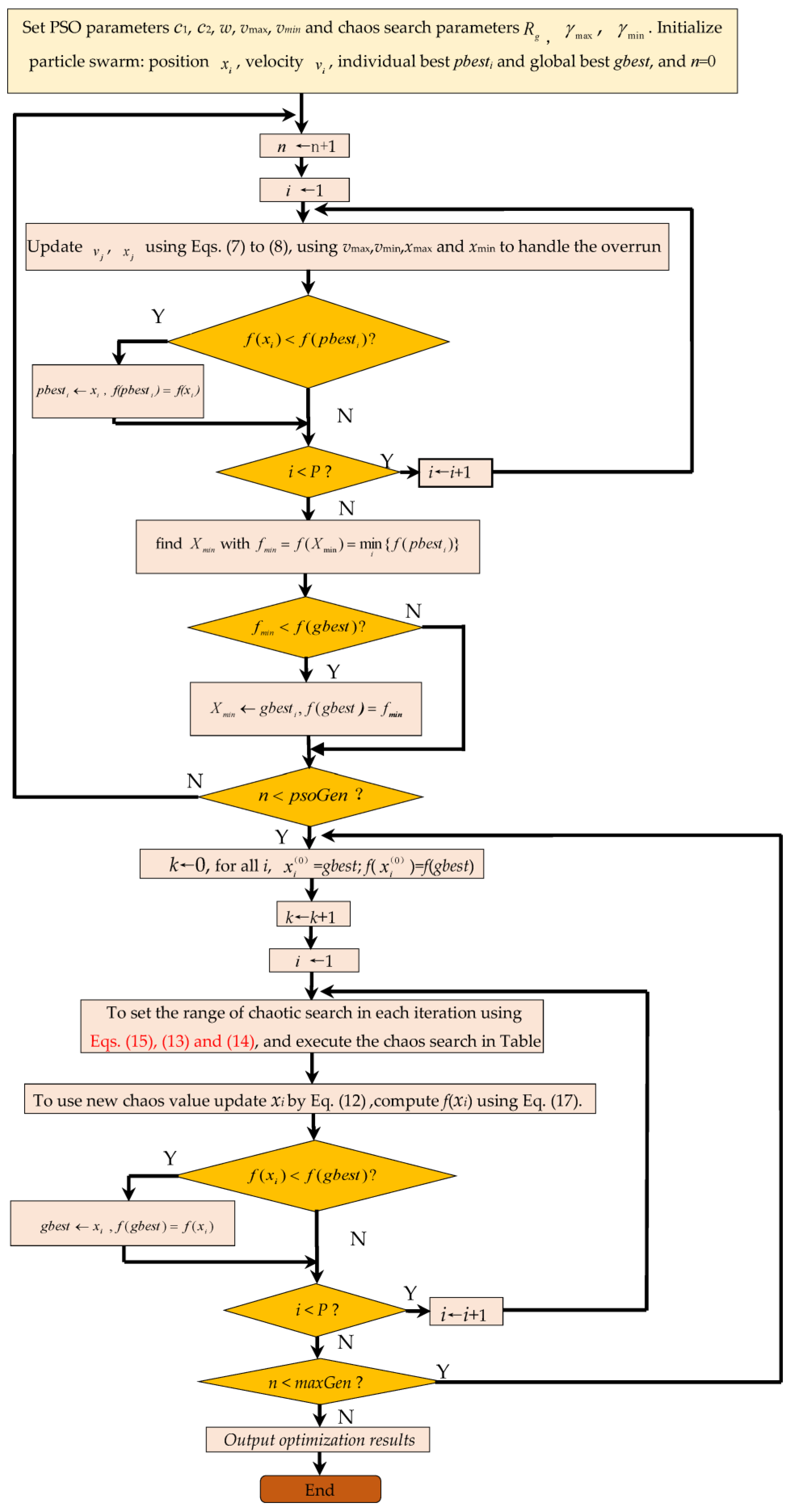
Algorithm 1. Matrix-version of PSO-VDCOA.

Set parameters: dimension dS, swarm size pS, coefficients c1, c2, inertia weight w, total iteration generations maxGen, PSO iteration generations psoGen; position limit: xmax and xmin; velocity limit: vmax and vmin, Rg, γmax, γmin. Let k = 0. Initialize swarm: x = xmin + rand(pS, dS).*(xmax − xmin); Compute the fitness: FF = f(x); Pbest = x; fPbest = FF, fmin = min(fPbest), gbest = xmin, (xmin corresponding to fmin). Gbest = [gbest; gbest, …, gbest]T.  //totally pS rows for iter = 1 to maxGen do

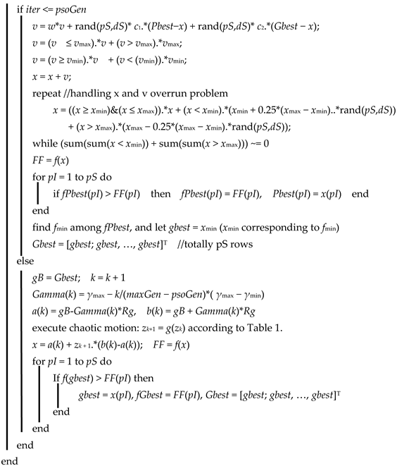
4. Simulation Experiments

A wireless sensor network is taken to verify the proposed method. It includes 30 sensor nodes distributed in a 20 m × 20 m monitoring region. The perceptive radius is $r_e=1.25$ m, the sensing radius is $r_s=2r_e=2.5$ m, and the node probability model coefficients are set as ${\lambda }_1=1$, ${\lambda }_2=0$, ${\beta }_1=1$, ${\beta }_2=1.5$, and $C_{th}=0.6$. The size of particle swarm: pS = 30, w = 0.7, ${\gamma }_{\max }$ = 1, ${\gamma }_{\min }$ = 0.9, $R_g$ = 0.1, $C_1=C_2=2$, and w_min = 0.5, w_max = 0.9 (LdiwPSO).

The total iteration number is 800, with the iteration generations of PSO and VDCOA being 300 and 500, respectively. The simulation program of six version of PSO-VDCOA are all completed with the same parameters, meanwhile, the CPSO, PSO and LdiwPSO algorithms are also programmed for the comparison. For fair comparison, all the nine algorithms employ the same randomly-created initial swarm and use the same iteration generation number (also the same function evaluation times). An initial swarm is created as shown in Figure 3, and its evenness value U₀ = 0.7753, coverage rate C₀ = 0.7169. After 800 generations of iterations, the optimized distributions achieved by CPSO, PSO, LdiwPSO and six PSO-VDCOA versions are shown in Figure 3 and Figure 4. The indexes of nine algorithms are presented in

Table 2. Numerical results of nine algorithms to solve wireless sensors coverage of the square region.

Algorithm	Coverage Rate C	Relative Ratio of Coverage Rate C/C0	Average Moving Distance (m)	Computing Time (s)
PSO-Circle	0.9444	1.3467	11.1881	253.5560
PSO-Logistic	0.9372	1.3363	10.4060	252.4002
PSO-Gaussian	0.9328	1.3301	10.3102	249.2707
PSO-Chebyshev	0.9089	1.2961	10.2535	249.5167
PSO-Sinusoidal	0.9306	1.3270	10.3612	253.5338
PSO-Cubic	0.9317	1.3286	10.6821	250.6576
LdiwPSO	0.9385	1.3383	9.9958	251.2138
PSO	0.9127	1.3015	9.9053	251.7490
CPSO	0.8038	1.1461	8.9682	253.6211

.

It can be concluded from the above figures and Table 2 that, under the same initial distribution and the same iteration number, the PSO-Circle, one version of PSO-VDCOA, was found to have the best sensors distribution, with the highest coverage rate of 0.9444, which corresponds to the highest relative ratio value of 1.3467. Considering the average moving distance index, the PSO-Circle is the worst one, which is because of its best coverage to inevitably need more moving distance to adjust the nodes positions. However, its average moving distance increment is about 2 m compared with the least average moving distance value of 8.9682 m. As for the computing time, the PSO-Circle runs 253.5560 s with only about 2 s more than others. To synthesize the above indexes, the PSO-Circle outperforms the other eight algorithms.

To further testify the adaptability of these algorithms, another case of rectangular region was also investigated. This region had a size of 25 m × 16 m, which is with the same area of 400 m² as the square region case. The parameters of the wireless sensors and the algorithms all remain unchanged. The simulation test was still completed, with 800 generations of iteration; the results are shown in Figure 5 and Figure 6, and

Table 3. Numerical results of four algorithms to solve wireless sensors coverage in the rectangle region.

Algorithm	Coverage Rate C	Relative Ratio of Coverage Rate C/C0	Average Moving Distance (m)	Computing Time (s)
PSO-Circle	0.9438	1.2948	9.9614	240.0654
PSO-Logistic	0.9433	1.2942	9.9669	240.1280
PSO-Gaussian	0.9422	1.2926	10.3507	243.1568
PSO-Chebyshev	0.9192	1.2610	10.5988	239.6768
PSO-Sinusoidal	0.9421	1.2925	9.7804	240.9370
PSO-Cubic	0.9415	1.2916	10.5918	242.2828
LdiwPSO	0.9420	1.2924	5.3234	241.4363
PSO	0.9197	1.2617	5.2271	239.4996
CPSO	0.8036	1.1025	4.1400	242.8174

. It can be seen from these figures and Table 3 that, under the same iteration number, PSO-VDCOA found the best sensors distribution, with the highest coverage rate of 0.9438, which indicates that the algorithm has better adaptability. The best effect is still achieved by the PSO-Circle. Its average moving distance and computing time also keep the same level as other algorithms without too great of an increase.

Finally, a more difficult circular case is tested. The circular region had a radius of 11.28m to retain the same area as the above two cases. The simulation setting also stayed the same as those of the above two cases; the results are shown Figure 7 and Figure 8 and

Table 4. Numerical results of nine algorithms to solve coverage in the circular region.

Algorithm	Coverage Rate C	Relative Ratio of Coverage Rate C/C0	Average Moving Distance (m)	Computing Time (s)
PSO-Circle	0.9190	1.3577	4.7833	234.7328
PSO-Logistic	0.8384	1.2386	4.4619	237.3758
PSO-Gaussian	0.8792	1.2989	4.8718	238.1806
PSO-Chebyshev	0.8552	1.2634	4.7083	231.7538
PSO-Sinusoidal	0.8907	1.3158	4.2943	235.2170
PSO-Cubic	0.9174	1.3553	4.4186	230.4234
LdiwPSO	0.9137	1.3498	5.3896	234.5706
PSO	0.7896	1.1665	4.8956	232.8963
CPSO	0.7511	1.1096	5.4600	233.0806

. All the algorithms show the performance deterioration; however, the PSO-Circle, as well as PSO_Cubic and LdiwPSO, still remained over 90% with better stability, and the former still keeps the highest.

To sum up the three cases of square, rectangular and circular regions, although they have the same area, the coverage rate obtained by optimization is different. The square one has the best coverage. The circular one is hard to optimize with the worst coverage, and six of the nine algorithms are not able to reach a 90% coverage rate, because these algorithms appeared to have premature convergence and fell into local optimums. PSO-Circle, PSO-Cubic and LdiwPSO all avoided the premature convergence and attain results over 91%, and PSO-Circle got the best coverage in the circular case, as well as the other two cases. PSO-Circle had the best improvement by increasing the coverage rate by 3.17%, 2.41% and 12.94% compared with PSO in three cases, respectively. Additionally, the average moving distance and computing time index of PSO-Circle are not distinctly more than other algorithms. Inspecting the procedures or flowchart of PSO-VDCOA, it has the same complexity and function evaluation times as the other algorithms. Therefore PSO-Circle is suggested to be the final selected algorithm for the coverage optimization of WSNs.

5. Conclusions

In this article, we presented a particle swarm and chaos combined method (PSO-VDCOA) for the coverage optimization of wireless sensor networks. This method can synthetically take advantage of PSO and VDCOA. The detailed realizations, particularly a new matrix-version, are presented. The simulation experiments of WSNs coverage optimization in three cases of square, rectangular and circular regions are completed to testify to the proposed algorithm; the optimization results demonstrated that the proposed algorithm is of high efficiency. The PSO-Circle, as one of the PSO-VDCOA versions, outperforms the other eight algorithms, and it can be selected for the practical coverage optimization for WSNs. Future research will be on the multi-objective optimization and constrained optimization of the coverage and energy-saving of WSNs based on the PSO-VDCOA.

References

1. Akyildiz, I.F.; Su, W.; Sankarasubramaniam, Y.; Cayirci, E. A Survey on Sensor Networks. IEEE Commun. Mag. 2002, 40, 102–114. [Google Scholar] [CrossRef] [Green Version]
2. Piromalis, D.; Arvanitis, K. Radio Frequency Identification and Wireless Sensor Networks Application Domains Integration Using DASH7 Mode 2 Standard in Agriculture. Int. J. Sustain. Agric. Manag. Inform. 2015, 1, 178. [Google Scholar] [CrossRef]
3. Qadir, J.; UIlah, U.; de Abajo, B.S.; Zapirain, B.G. Energy-Aware and Reliability Based Localization-Free Cooperative Acoustic Wireless Sensor Networks. IEEE Access 2020, 8, 121366–121384. [Google Scholar] [CrossRef]
4. Borja, B.; Carlos, M.; Ramón, A.; Tomás, R. A Hardware-Supported Algorithm for Self-Managed and Choreographed Task Execution in Sensor Networks. Sensors 2018, 18, 812. [Google Scholar]
5. Ghosha, A.; Dasb, S.K. Coverage and Connectivity Issues in Wireless Sensor Networks: A Survey. Pervasive Mob. Comput. 2008, 4, 303–334. [Google Scholar] [CrossRef]
6. Wang, D.; Xie, B.; Agrawal, D.P. Coverage and Lifetime Optimization of Wireless Sensor Networks with Gaussian Distribution. IEEE Trans. Mob. Comput. 2008, 7, 1444–1458. [Google Scholar] [CrossRef]
7. Jia, J.; Chen, J.; Chang, G.; Wen, Y.; Song, J. Multi–objective Optimization for Coverage Control in Wireless Sensor Network with Adjustable Sensing Radius. Comput. Math. Appl. 2009, 59, 1767–1775. [Google Scholar] [CrossRef] [Green Version]
8. Guo, Y.; Liu, D.; Chen, M.; Liu, Y. An Energy–efficient Coverage Optimization Method for Wireless Sensor Networks Based on Multi–objective Quantum–inspired Cultural Algorithm. In Proceedings of the ISNN’13: Proceedings of the 10th international conference on Advances in Neural Networks, Dalian, China, 4–6 July 2013; Springer: Berlin/Heidelberg, Germany, 2013; p. 349. [Google Scholar]
9. Wang, L.; Wu, W.; Qi, J.; Jia, Z. Wireless Sensor Network Coverage Optimization Based on Whale Group Algorithm. Comput. Sci. Inf. Syst. 2018, 15, 569–583. [Google Scholar] [CrossRef] [Green Version]
10. Deepa, A.; Venkataraman, R. Enhancing Whale Optimization Algorithm with Levy Flight for Coverage Optimization in Wireless Sensor Networks. Comput. Electr. Eng. 2021, 94, 107359. [Google Scholar] [CrossRef]
11. Khalaf, O.I.; Abdulsahib, G.M.; Sabbar, B.M. Optimization of Wireless Sensor Network Coverage Using the Bee Algorithm. J. Inf. Sci. Eng. 2020, 36, 377–386. [Google Scholar]
12. Roselin, I.; Latha, P. Energy Efficient Coverage Using Artificial Bee Colony Optimization in Wireless Sensor Networks. J. Sci. Ind. Res. 2016, 75, 19–27. [Google Scholar]
13. Zhu, F.; Wang, W. A Coverage Optimization Method for WSNs Based on the Improved Weed Algorithm. Sensors 2021, 21, 5869. [Google Scholar] [CrossRef] [PubMed]
14. Wang, S.; You, H.; Yue, Y.; Cao, L. A Novel Topology Optimization of Coverage-oriented Strategy for Wireless Sensor Networks. Int. J. Distrib. Sens. Netw. 2021, 17, 155014772199229. [Google Scholar] [CrossRef]
15. Aca, B.; Ddb, C. Energy-efficient Coverage Optimization in Wireless Sensor Networks Based on Voronoi-Glowworm Swarm Optimization-K-Means Algorithm. Ad Hoc Netw. 2021, 122, 102660. [Google Scholar]
16. Chowdhury, A.; De, D. Fis-rgso: Dynamic Fuzzy Inference System Based Reverse Glowworm Swarm Optimization of Energy and Coverage in Green Mobile Wireless Sensor Networks. Comput. Commun. 2020, 163, 12–34. [Google Scholar] [CrossRef]
17. Cao, L.; Yue, Y.; Cai, Y.; Zhang, Y. A Novel Coverage Optimization Strategy for Heterogeneous Wireless Sensor Networks Based on Connectivity and Reliability. IEEE Access 2021, 9, 18424–18442. [Google Scholar] [CrossRef]
18. Ding, Y.S.; Lu, X.J.; Hao, K.R.; Li, L.F.; Hu, Y.F. Target Coverage Optimisation of Wireless Sensor Networks Using a Multi-Objective Immune Co-evolutionary Algorithm. Int. J. Syst. Sci. 2011, 42, 1531–1541. [Google Scholar] [CrossRef]
19. Xenakis, A.; Foukalas, F.; Stamoulis, G.; Katsavounidis, I. Topology Control with Coverage and Lifetime Optimization of Wireless Sensor Networks with Unequal Energy Distribution. Comput. Electr. Eng. 2017, 64, 182–199. [Google Scholar] [CrossRef]
20. Lee, J.W.; Choi, B.S.; Lee, J.J. Energy-efficient Coverage of Wireless Sensor Networks Using Ant Colony Optimization with Three Types of Pheromones. IEEE Trans. Ind. Inform. 2017, 7, 419–427. [Google Scholar] [CrossRef]
21. Binh, H.T.T.; Hanh, N.T.; Van Quan, L.; Dey, N. Improved Cuckoo Search and Chaotic Flower Pollination Optimization Algorithm for Maximizing Area Coverage in Wireless Sensor Networks. Neural Comput. Appl. 2018, 30, 2305–2317. [Google Scholar] [CrossRef]
22. Gupta, G.P.; Jha, S. Biogeography-based Optimization Scheme for Solving the Coverage and Connected Node Placement Problem for Wireless Sensor Networks. Wirel. Netw. 2019, 25, 3167–3177. [Google Scholar] [CrossRef]
23. Miao, Z.; Yuan, X.; Zhou, F.; Qiu, X.; Chen, K. Grey Wolf Optimizer with an Enhanced Hierarchy and Its Application to the Wireless Sensor Network Coverage Optimization Problem. Appl. Soft Comput. 2020, 96, 10660. [Google Scholar] [CrossRef]
24. Zhang, Y.; Cao, L.; Yue, Y.; Cai, Y.; Hang, B. A Novel Coverage Optimization Strategy Based on Grey Wolf Algorithm Optimized by Simulated Annealing for Wireless Sensor Networks. Comput. Intell. Neurosci. 2021, 2021, 6688408. [Google Scholar] [CrossRef] [PubMed]
25. Subramanian, K.; Shanmugavel, S. A Complete Continuous Target Coverage Model for Emerging Applications of Wireless Sensor Network Using Termite Flies Optimization Algorithm. Wirel. Pers. Commun. 2021, 1–23. [Google Scholar] [CrossRef]
26. Sun, Z.; Shu, Y.; Xing, X.; Wei, W.; Song, H.; Li, W. Lpocs: A Novel Linear Programming Optimization Coverage Scheme in Wireless Sensor Networks. Ad Hoc Sens. Wirel. Netw. 2016, 33, 173–197. [Google Scholar]
27. Mostafaei, H.; Meybodi, M.R. An Energy Efficient Barrier Coverage Algorithm for Wireless Sensor Networks. Wirel. Pers. Commun. 2014, 77, 2099–2115. [Google Scholar] [CrossRef]
28. Zhang, H.H.; Jennifer, C.; Hou, J. Maintaining Sensing Coverage and Connectivity in Large Sensor Networks. J. Wirel. Ad Hoc Sens. Netw. 2005, 1, 89–123. [Google Scholar]
29. Tarnaris, K.; Preka, I.; Kandris, D.; Alexandridis, A. Coverage and K-coverage Optimization in Wireless Sensor Networks Using Computational Intelligence Methods: A Comparative Study. Electronics 2020, 9, 675. [Google Scholar] [CrossRef] [Green Version]
30. Shi, Y.; Eberhart, R.A. Modified Particle Swarm Optimizer. In Proceedings of the IEEE International Conference on Evolutionary Computation Proceedings, Anchorage, AK, USA, 4–9 May 1998. [Google Scholar]
31. Wang, X.; Wang, S.; Ma, J.J. An Improved Co–evolutionary Particle Swarm Optimization for Wireless Sensor Networks with Dynamic Deployment. Sensors 2007, 7, 354–370. [Google Scholar] [CrossRef] [Green Version]
32. Sun, H.; Li, J.; Wang, H. A Hybrid Particle Swarm Optimization for Wireless Sensor Network Coverage Problem. Sens. Lett. 2012, 10, 1744–1750. [Google Scholar] [CrossRef]
33. Wang, Y.; Li, M. Coverage Control Optimization Algorithm for Wireless Sensor Networks Based on Combinatorial Mathematics. Math. Probl. Eng. 2021, 2021, 6066379. [Google Scholar] [CrossRef]
34. Zhang, Y.; Sun, X.; Yu, Z. K-barrier Coverage in Wireless Sensor Networks Based on Immune Particle Swarm Optimization. Int. J. Sens. Netw. 2018, 27, 250–258. [Google Scholar] [CrossRef]
35. Bai, X.; Li, S.; Xu, J. Mobile Sensor Deployment Optimization for K-coverage in Wireless Sensor Networks with a Limited Mobility Model. IETE Tech. Rev. 2010, 27, 124–137. [Google Scholar] [CrossRef]
36. Xu, Y.; Ding, O.; Qu, R.; Li, K. Hybrid Multi-objective Evolutionary Algorithms Based on Decomposition for Wireless Sensor Network Coverage Optimization. Appl. Soft Comput. 2018, 68, 268–282. [Google Scholar] [CrossRef] [Green Version]
37. Wang, X.; Ma, J.J.; Sheng, W.; Bi, D.W. Distributed Particle Swarm Optimization and Simulated Annealing for Energy-efficient Coverage in Wireless Sensor Networks. Sensors 2007, 7, 628–648. [Google Scholar] [CrossRef] [Green Version]
38. Shi, Y.H.; Eberhart, R.C. Empirical Study of Particle Swarm Optimization. In Proceedings of the Congress on Evolutionary Computation, Washington, DC, USA, 6–9 July 1999. [Google Scholar]
39. Eberhart, R.C.; Shi, Y.H. Comparing Inertia Weights and Constriction Factors in Particle Swarm Optimization. In Proceedings of the IEEE Congress on Evolutionary Computation, La Jolla, CA, USA, 16–19 July 2000. [Google Scholar]
40. Clerc, M.; Kennedy, J.E. The Particle Swarm–explosion, Stability in a Multidimensional Complex Space. IEEE Trans. Evol. Comput. 2002, 6, 259–267. [Google Scholar] [CrossRef] [Green Version]
41. Sekikawa, M.; Kousaka, T.; Tsubone, T.; Inaba, N.; Okazaki, H. Bifurcation Analysis of Mixed-mode Oscillations and Farey Trees in an Extended Bonhoeffer–Van Der Pol Oscillator. Phys. D Nonlinear Phenom. 2022, 433, 133178. [Google Scholar] [CrossRef]
42. Ahmad, J.; Hwang, S.O. Chaos-based Diffusion for Highly Autocorrelated Data in Encryption Algorithms. Nonlinear Dyn. 2015, 82, 1839–1850. [Google Scholar] [CrossRef]
43. Yuan, X.; Zhang, T.; Xiang, Y.; Dai, X. Parallel Chaos Optimization Algorithm with Migration and Merging Operation. Appl. Soft Comput. 2015, 35, 591–604. [Google Scholar] [CrossRef]
44. Kohli, M.; Arora, S. Chaotic Grey Wolf Optimization Algorithm for Constrained Optimization Problems. J. Comput. Des. Eng. 2018, 5, 458–472. [Google Scholar] [CrossRef]
45. Tavazoei, M.S.; Haeri, M. Comparison of Different One-dimensional Maps as Chaotic Search Pattern in Chaos Optimization Algorithms. Appl. Math. Comput. 2007, 187, 1076–1085. [Google Scholar] [CrossRef]
46. Jiang, C.; Bompard, E.A. Hybrid Method of Chaotic Particle Swarm Optimization and Linear Interior for Reactive Power Optimisation. Math. Comput. Simul. 2005, 68, 57–65. [Google Scholar]
Figure 1. Six different chaotic maps. (a) Circle. (b) Logistic. (c) Gaussian. (d) Chebyshev. (e) Sinusoidal. (f) Cubic.
Electronics 11 00853 g001aElectronics 11 00853 g001b
Figure 2. Flowchart of PSO-VDCOA.
Electronics 11 00853 g002
Figure 3. Random initialization of sensors positions and the convergence graphs for the square region coverage. (a) Initial random distribution of sensors (b) Converge curves of nine algorithms (c) Local magnified view of figure (b).
Electronics 11 00853 g003
Figure 4. Final sensor deployment of nine algorithms to solve wireless sensors coverage in a square region. (a) PSO-Circle. (b) PSO-Logistic. (c) PSO-Gaussian. (d) PSO-Chebyshev. (e) PSO-Sinusoidal. (f) PSO-Cubic. (g) LdiwPSO. (h) PSO. (i) CPSO.
Electronics 11 00853 g004aElectronics 11 00853 g004b
Figure 5. Random initialization of sensors positions and the convergence graphs for the rectangular region coverage. (a) Initial random distribution of sensors (b) Converge curves of nine algorithms (c) Local magnified view of figure (b).
Electronics 11 00853 g005
Figure 6. Results of nine algorithms to solve wireless sensors coverage in a rectangular region. (a) PSO-Circle. (b) PSO-Logistic. (c) PSO-Gaussian. (d) PSO-Chebyshev. (e) PSO-Sinusoidal. (f) PSO-Cubic. (g) LdiwPSO. (h) PSO. (i) CPSO.
Electronics 11 00853 g006
Figure 7. Random initialization of sensors positions and the convergence graphs for the circular region coverage. (a) Initial random distribution of sensors (b) Converge curves of nine algorithms (c) Local magnified view of figure (b).
Electronics 11 00853 g007
Figure 8. Results of nine algorithms to solve wireless sensors coverage in a circular region. (a) PSO-Circle. (b) PSO-Logistic. (c) PSO-Gaussian. (d) PSO-Chebyshev. (e) PSO-Sinusoidal. (f) PSO-Cubic. (g) LdiwPSO. (h) PSO. (i) CPSO.
Electronics 11 00853 g008