1. Introduction
Violence recognition is a sub-area of human action recognition that can be divided between internal and external environments [
1]. This is a crucial distinction, as the issues and problems to be addressed in these two types of environments are quite different. For example, it is generally not feasible to include the audio signal in outdoor surveillance, but it can be included indoors. Internal surveillance, where the capture and adequate audio signal filtering is straightforward, can help obtain better results [
2]. These audio and video signals can go through a multimodal fusion process to increase the success rate [
3].
When studying the recognition of violence, the most common data are related to the video. Nevertheless, recent studies also include audio since microphones can easily pick up audio, being very powerful sensors that capture context and human behaviour [
2]. However, the recognition of violence through audio is highly susceptible to significant fluctuations in the accuracy, depending on the acoustic environment in which it is inserted. Therefore, it is necessary to have a good audio representation to perform the audio-based violence classification.
Some computational complexity is required when we try to detect violence that manifests itself across space and time: space refers to the amount of memory used to store data during and after an algorithm runs; time refers to the number of processing instructions performed by a computer [
4,
5]. In addition to the computational complexity, a temporal restriction corresponds to the processing that exceeds the deadline foreseen in real-time [
6,
7]. According to these restrictions, the hardware must be considered part of the detection model. Therefore, we have to detect and recognise violence with really short deadlines considering real-time surveillance. Since the sensor data are from inside the vehicle, the hardware installed is not very powerful, so the only parameter to be changed is the computational complexity.
An in-car surveillance system has two interlinked restrictions to consider in this article. The first is data protection, and the second is that as much surveillance as possible should be automatic so that only an event that calls an operator is triggered if violence is recognized [
2]. This means that processing must be carried out inside the vehicle, without data storage and in real-time. Furthermore, the hardware should not be expensive enough to be worth stealing. This imposes several hardware constraints that can be summarized as surveillance must be optimized for as little computational complexity as possible [
1].
Deep neural networks have achieved tremendous success; however, these models can be vulnerable. In this way, models can be easily fooled with small, inconspicuous changes. These elaborate inputs, also known as adversarial examples, posed a significant challenge for researchers to build secure and robust models for security-sensitive applications [
8].
Since Szegedy [
9], the existence of adversarial examples in deep models have been studied, and many efforts have been made to improve the models’ resistance against such attacks. Examples of these attacks are opponent training [
8], gradient regularization [
8] and data pre-processing [
8]. Still, it is difficult to build a robust and adversarial model. The model must have an appropriate defence and, in addition to dealing with various types of attacks, it must also avoid using “external” factors, such as gradient mask or blurred gradients [
8], to build a false sense of security.
1.1. Main Contributions
This paper results from a cooperation between the University of Minho and the Bosch Group. The cooperation aims to a violence detection surveillance system to be used inside vehicles, especially on car-pooling services, (e.g., Uber, Lynx, etc.). For such a task for the video signal, several architectures were evaluated, and those that presented the best performance are X3D, C2D, and I3D [
10]. Given the proposed models are presenting good performance, the surveillance intuition says that the next step is to test them against security threats. That is the context for this paper.
Notice that the main contribution is the application context. The result of X3D, C2D and I3D as well their security limitations are already known, but in a lato sense [
11]. On the other hand, few papers are focusing in-vehicle surveillance (perhaps due to the novelty of the field), as can be observed by the lack of suitable public data-sets [
12]. Surveillance, being a sensitive issue, cannot be discussed “in general” but in strict terms. This paper’s objective is to assess strictly how does X3D, C2D and I3D applied to in-vehicle surveillance behaves on adversarial attacks and discusses how reliable such a solution is to be used as violence detection on car-pooling services. This paper contribution is, to the best of the author’s knowledge, this is first one to perform the frame and video level evaluation to in-car violence recognition models.
Violence can be triggered by several sources, from emotion-driven to malicious action. The scenario for this paper focuses on malicious actions. An adversarial enters into a shared car using a signal jammer (for a reference, visit
https://www.jammerall.com/ access at 5 December 2021) that adds noise to the video signal while the malicious action takes place. The research question that arises is: does the proposed architectures are robust enough for coping with such attack?
Building a robust model adversarial has to effectively and reasonably assess the opposing robustness of deep models. A practical assessment procedure helps investigators understand the different defence methods. The most used and evaluated current methods are FGSM [
13], PGD [
14], and C&W attacks [
15].
1.2. Organization
Being an extended version of the paper [
10], the aim is to present the weakness of in-car violence recognition models, which is based on the paper [
10]. The research objective is to evaluate the weakness of deep learning models for violence detection inside the vehicle. The research is currently at an early stage when explorations are being undergone, and feasibility is being evaluated.
The remainder of this paper is structured as follows: In
Section 2, the main works are related to the theoretical foundations.
Section 3 presents an analysis of the dataset and architectures. In
Section 4, we describe the results and discussion.
Section 5 presents the conclusions and future works.
2. Theoretical Foundations
2.1. Adversarial Attacks
Although the deep learning models have achieved expressive results in the most varied domains [
16], even getting better performance than the human being in specific tasks [
17]. The work of advatk has shown that these models have intriguing properties that go against our intuition. These works showed that the models fail drastically if we add an almost imperceptible amount of noise to the human eye in an image.
Examples of these attacks are opponent training [
8], gradient regularization [
8] and data pre-processing [
8]. Still, it is difficult to build a robust and adversarial model. The model must have an appropriate defence and, in addition to dealing with various types of attacks, it must also avoid using “external” factors, such as gradient mask or blurred gradients [
8], to build a false sense of security.
2.1.1. Adversarial Training
Inkawhich et al. [
18] proposed the
Fast Gradient Sign Method (FGSM) for generating adversarial attacks. FGSM consists of calculating the gradient of the error function concerning the input vector and then obtaining the signs (direction) of each dimension of the gradient vector. The author [
19] argue that the direction of the gradient is more important than the specific point of the gradient because the space in which the input vector is contained is not composed of adversary attack subregions. Other variations of the FGSM are also present in the literature, such as the R-FGSM [
20] and Step-LL [
21]. Equation (
1) presents a cost function for adversarial training based on the FGSM. Given a standard error function (
J) and the input vector
x, it gets the final error based on the sum of two steps: (1) calculates the error based on the original input vector (
); and (2) error based on FGSM opponent attack (
).
Madry et al. [
14] carried out a study on opposing attacks from a
view in order to be precise about which attack class they try to recognize and, consequently, defend. Equation (
2) presents the formulation
. The
part of this formulation aims to find an adversary noise that produces a high value of the error function
L when added to the input vector. The term o
aims to find the model parameters that minimize the
L error function, thus making the model robust to
. From this analysis, the authors proposed the
Projected Gradient Descent (PGD) method, which they call the first-order universal attack, that is, the most difficult attack using only first-order information.
Although the PGD method achieves good results, it is computationally expensive because it needs to calculate the function’s gradient several times. In an effort to mitigate this restriction, Ref. [
22] proposed the method
Free Adversarial Training (FAT). The main contribution of the FAT method is to reuse the computed function gradient when the model performs the gradient descent in the optimization step. However, with just one step of the gradient calculation, they cannot build an attack that causes an error as high as PGD. To minimize this negative point, the authors propose to train the same input
batch for
m times. In this way, the model will be robust to more than one attack version for the same input vector.
2.1.2. Interpretability Methods
Deconvolution [
23] is the pioneering work in obtaining the interpretations of a deep learning model following a
top-down approach. It can be seen as a traditional convolutional neural network using the same components (filters,
pooling), but in reverse order. Deconvolution [
23] is almost equivalent to calculating the gradient of the output of an arbitrary neuron concerning the input vector (
Vanilla Gradient); the subtle difference is that when the signal is back-propagated through an ReLU function, it sets to zero each negative value of the previous gradient. Following a more formal approach, the Vanilla Gradient [
24,
25] method was proposed. This method obtains a heatmap containing the degree of importance of each position of the input vector
x. Given a position
i of a layer
f, the absolute value of the gradient
is calculated to obtain the importance of each position of
x. The
Guided Backpropagation [
26] method combines the Deconvolution and Vanilla Gradient methods, setting to zero the values in the positions where the gradients or the forward positions of the respective layer are negative.
There are other computationally more complex interpretation methods, such as GradCam [
27], Guided GradCam [
27], Integrated Gradients [
28], Blur Integrated Gradients [
29], Deep Lift [
30], Kernel Shap [
31], among others. However, due to computational limitations, we will only focus on these gradient-based ones more directly.
2.2. Architectures
2.2.1. X3D
The X3D (Expand 3D) architecture requires low computational power for its processing. This way allows us to have the precision to perform violence recognition with computers without great computational powers. Furthermore, the X3D architecture extends a small 2D imaging architecture towards a Spatio-temporal architecture by extending several potential axes. It develops the idea of adding axes (inflation as in I3D) and applying them in different steps. Progressively expands a 2D network from the axes: time, frequency, space, width, bottleneck and depth, resulting in architecture to extend from 2D space to the field of 3D spacetime. The architecture describes a basic set of extension operations used to sequentially extend X2D from a short spatial network to X3D, a spatiotemporal network, implementing the following operations on the temporal, spatial, width and depth dimension [
11].
2.2.2. C2D
A Two-Dimensional Convolutional Neural Network (C2D) [
32] is a structure composed of two steps: (1) learning parameters; and (2) classification. The first step is to reduce an initial two- or three-dimensional structure to a one-dimensional structure to be passed to a neural classifier. Roughly speaking, if such reduction is made directly, as:
=>|100010| the spatial dependence of pixels is eventually lost. To avoid this, the alternative explored by CNN is convolutions interspersed by pooling. The second step consists of a classification process as it is traditionally done through neural networks. In this sense, CNN is suitable for processing images and sound (two-dimensional structures) and movies (sequences of two-dimensional structures). So we have a model based on convolutional networks and pooling layers. This model is finished with two full-connected layers and the Softmax function.
2.2.3. I3D
When adding a dimension in a C2D architecture (e.g.,
k ×
k), it becomes a C3D architecture (e.g.,
t ×
k ×
k) [
33]. The recognition of actions is sought through spatiotemporal analysis by adding one more axis (inflated) in 2D convolutional networks aiming to treat time. Inflate is not a simple C3D, but a C2D, usually pre-trained, whose grains are extended into a 3D shape. Growing up is as simple as adding dimension. Usually, temporal [
34] adds an extra dimension to all filters and kernels of a 2D convolutional model. I3D stands for a two-flow inflated 3D convolution network [
33]. Therefore, I3D is a composite of a C2D inflated with optical flow information [
33,
34].
3. Materials and Methods
The dataset is the cornerstone of this paper. Incar violence recognition is a challenging task. The violence phenomenon can be manifested in various ways. For example, it can be fast or slow, it may not have violent movement but has violent tools, it can be only a threat and not the physical violence itself, and other situations. Due to its difficulty level, preprocessing is a major step in the process because it can help the model focus on the violence signals. Thus, we have used several preprocessing functions, such as spatial sampling, temporal sampling, random horizontal flip, and normalization.
Since it was impossible to find a public data set focused on in-vehicle surveillance, one was generated specifically for this project. In short, the dataset is composed of 640 clips scattered for 20 scenarios and 16 pairs of actors. Some clips are enriched with objects such as a gun and a hairbrush. For details refer to [
35].
A breadth exploration on neural networks architectures for computer vision focused on action recognition revealed that X3D, C2D and I3D present good performance when applied for in-vehicle violence detection [
36]. These architectures also comply with the constraint of meeting real-time evaluation working on inexpensive hardware. After training various models and evaluating them with the test set, we configure all the systems in the car to test which model is the best in the real scenario. This testing step is one of the most important in the project. We could discover that the model has many false positives and is highly sensitive. Next, in order to solve this problem, we discuss options to discover what the issue is. Then, we discovered that training the models with the entire video was not a good decision because a violent video also has splits that do not have violence. Therefore, we decided to cut all violent videos in slices of 5 s and keep only the slices that have violent situations. In order to keep only the slices with violent behaviour, we re-watch all the slices and keep only the violent ones. After cutting all videos, we retrained all models with the new dataset, and the result was not highly sensitive and more accurate model in the deployed scenario.
The training is based on ten pairs of actors, validated on three and tested on the last three. Pre-processing was undertaken using spatial sampling, temporal sampling, random horizontal flip and normalization. After model stabilization and selection, a test set was generated modified by FGSM, PGD and CW and submitted for the X3D, C2D and I3D models to verify how assess their robustness.
4. Results and Discussion
4.1. Models Convergence
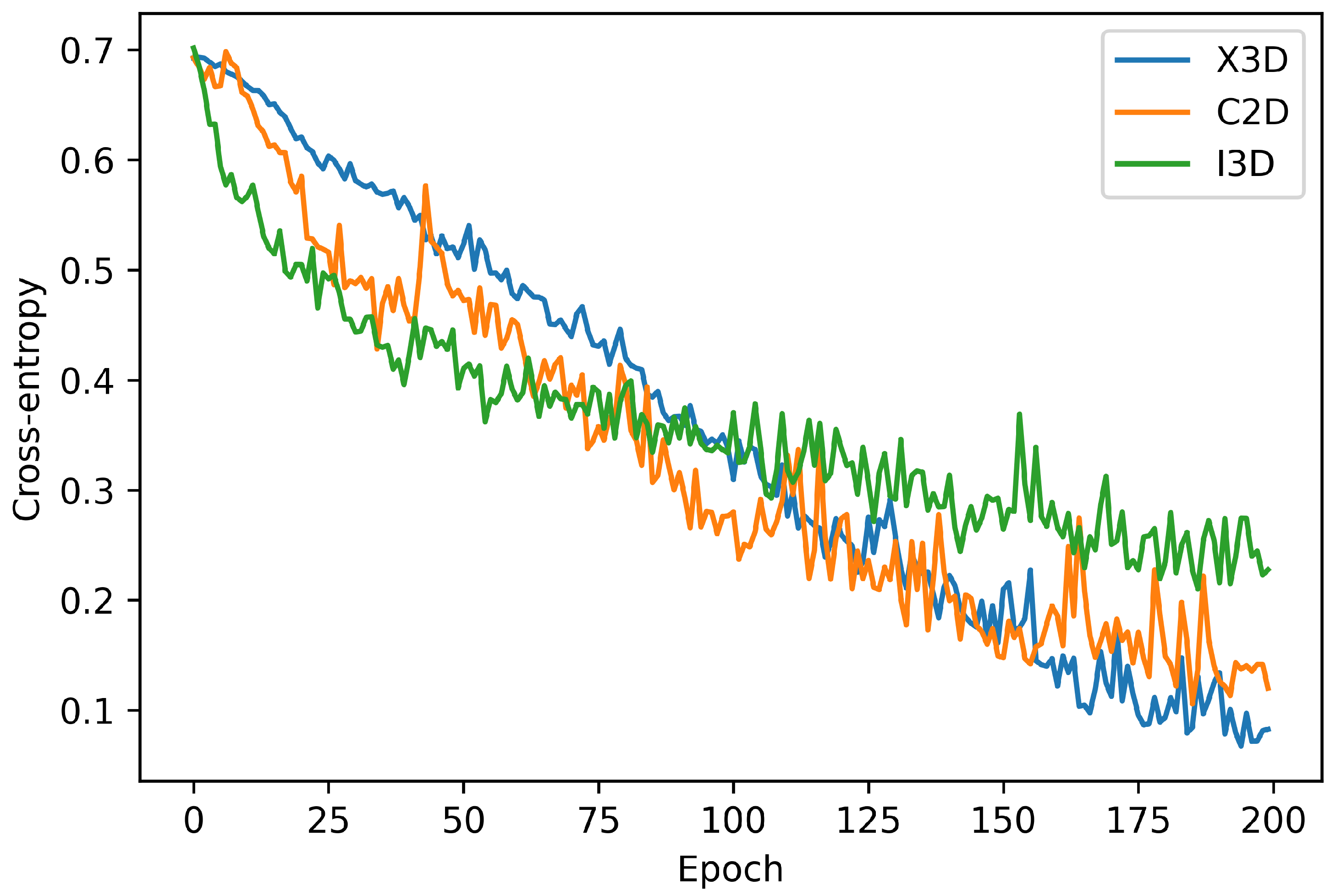
Visualizing the model loss behaviour for epoch is important to verify if the model is learning or is blocked in a local minimum. Thus, this subsection presents the model convergence during the training step. All the models were trained during 200 epochs, using the Adam optimizer with a learning rate 0.001 and batch size of 16 videos.
Figure 1 and
Figure 2 shows the training loss and accuracy for each epoch, respectively.
From
Figure 1 we can see that the X3D model has the most stable convergence, decreasing the loss by tiny steps. However, although the C2D and the I3D models achieved the lower loss in the first epochs, they did not present the lowest loss in the final epochs. Similar behaviour can be seen in
Figure 2 with the accuracy metric.
After training all models during 200 epochs, we selected the epoch with a lower loss value in the training set and evaluated it in the test set for each model. As the data set is unbalanced, we have employed the weighted f-measure metric in the test set evaluation.
Table 1 shows the test results obtained. The X3D architecture achieves the best results, and although the C2D achieve close loss training to the I3D, it achieves lower f-measure in the test set.
4.2. Adversarial Robustness
In the last subsection, we have made the model evaluation through the cross-entropy loss, accuracy, and f-measure metrics with the train and test set. Nevertheless, this standard evaluation only measures how the model predicts the training and testing data samples correctly; thus, a simple evaluation as the in-car violence signal can be presented in different ways. For example, it can be a fast or slow violence movement. The scene can be dark or lighter, only one or two people are moving, is necessary to employ a more in-depth analysis of the in-car violence recognition models. Thus, in this work, we have applied two well-known adversarial attack techniques to evaluate how sensible to adversarial attacks the in-car models FGSM and PGD.
The adversarial attack adds (imperceptible) noise to the input signal. Since the video is composed of a sequence of frames, we have made two levels of adversarial robustness evaluation: (i) video level and (ii) frame level. The first level consists of adding noise to all video frames, while in the second one, we add noise only to a single frame. These two levels of analysis are essential to verify the model weakness and sensibility regarding the complete video and in a frame-by-frame way.
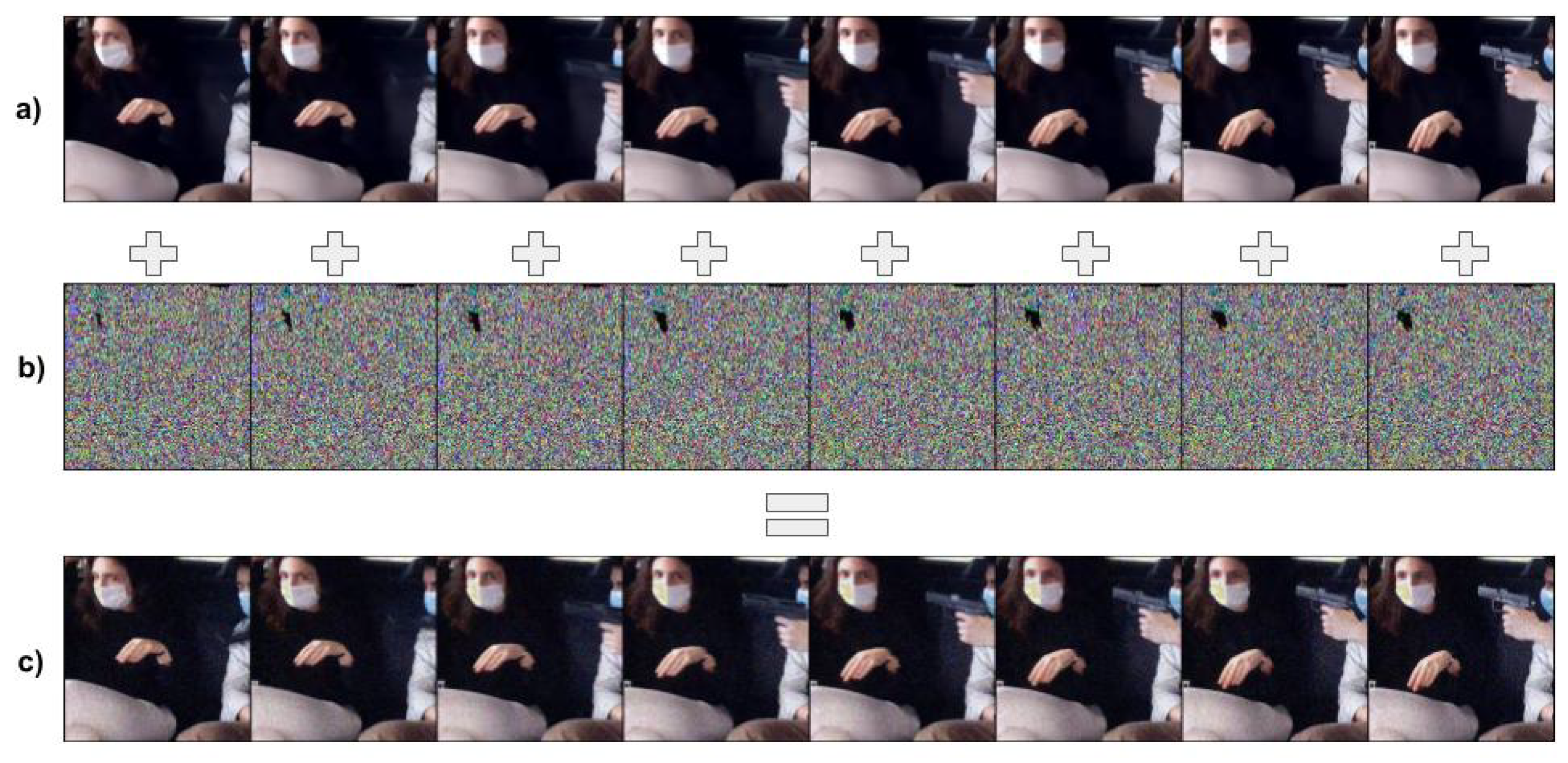
4.2.1. Video-Level
In this analysis, we add adversarial noise to each frame of the input feature; thus, all the video signal has adversarial, as represented in
Figure 3. In this example, the adversarial noise in the image (b) was obtained from the FGSM. However, it can be obtained from any other adversarial attack method. This level of analysis is essential to verify how adversarial robust is the in-car violence models regarding all the videos.
The standard evaluation has shown that the X3D model presented better results on the test set. Differently from these results,
Table 2 has shown that the I3D model achieved better results on the adversarial robustness with the video-level signal. This result reinforces the necessity to evaluate the model with other approaches different from the standard. Thus, the researchers can have different evaluation scenarios and infer the model weakness.
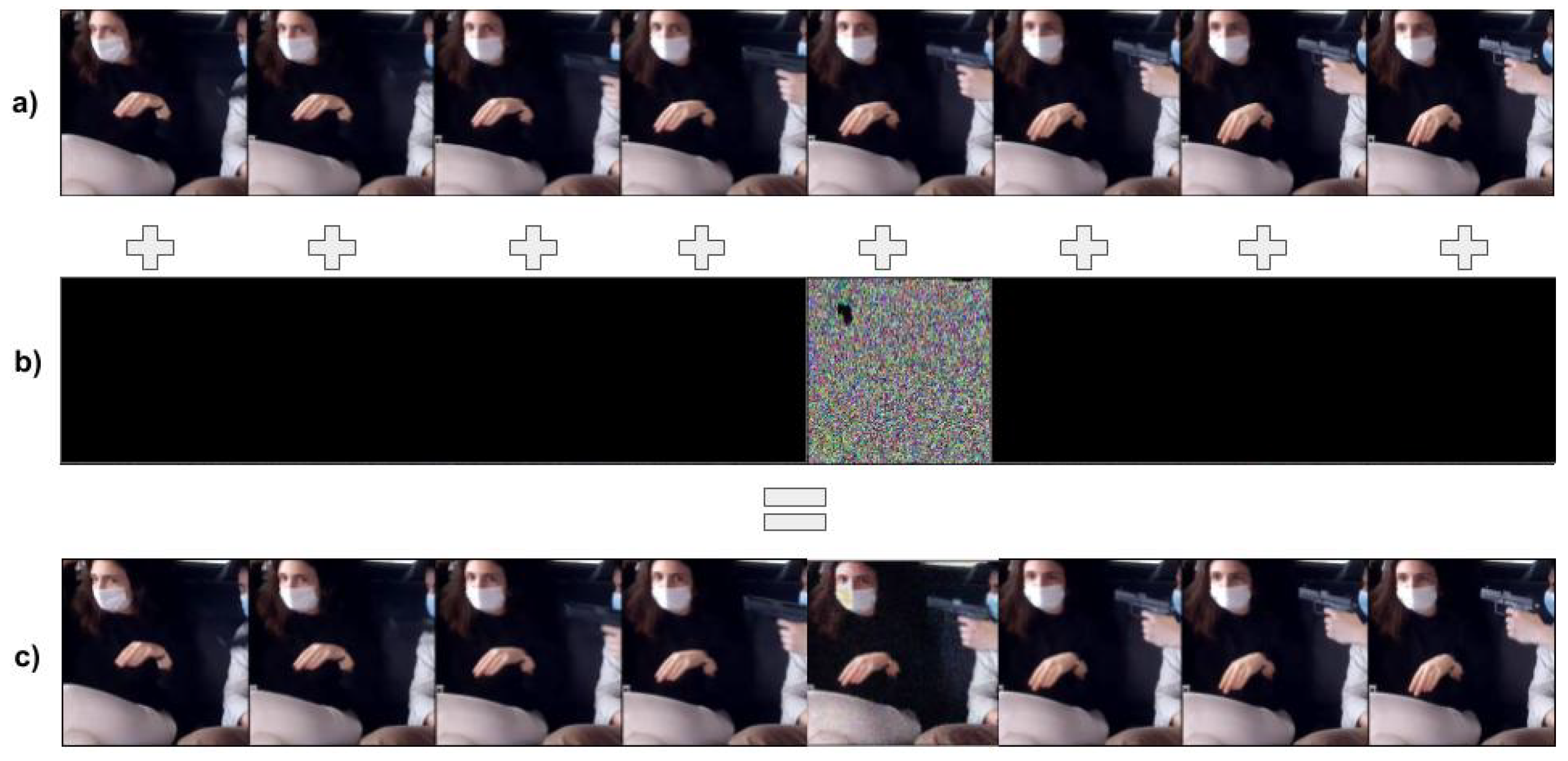
4.2.2. Frame-Level
During the frame-level analysis, we chose a single frame in the input video and added adversarial noise on it, as illustrated in
Figure 4. This example represents the process of adding FGSM adversarial noise on the fifth frame of the input video. This level of analysis is vital to verify if the model is adversarial robust to noise on a single frame.
Table 3 presents the results obtained in the frame-level analysis. The most adversarial robust model in a frame-level scenario was the I3D model, thus confirming that it is the most adversarial robust model between the ones evaluated. In addition, the X3D presented interesting results since it has close results to the I3D, but at the video level have lousy performance.
In addition to what we already have discussed, it is essential to highlight that the results presented in
Table 2 and
Table 3 have shown that all models have a drawback in the evaluation metrics when we add adversarial noise (even frame or video level). This fact is important because when we deploy in-car violence recognition models in production, some situations can happen, sometimes the camera point of view of even the camera resolution changes, so evaluating the model sensitivity is very important before deploying these models.
4.3. Sanity-Check Based on Interpretability
Interpretability methods produce attribution maps in the input space, meaning that each input feature is essential to the model prediction. Moreover, we can use these methods to perform sanity checks on the model’s outputs, thus inferring the model’s sensitivity to the input feature. In addition, we can also use interpretability methods to debug models prediction.
Video signal is composed of temporal and spatial information, and we can use the frame sequence as the temporal line and the spatial subregions of each frame as the spatial information. This section will perform sanity checks of the video signal based on the model interpretability from these signals. The sanity check consists of (1) erasing the most important temporal information and (2) erasing the most important spatial information. These sanity tests allow us to verify how sensitive is the model regarding input feature changes. This analysis is motivated by the work presented in [
36]. It is different from randomly erased subregions or frames because it uses interpretability methods to choose the most crucial frame or subregion. In the following, we present the results obtained.
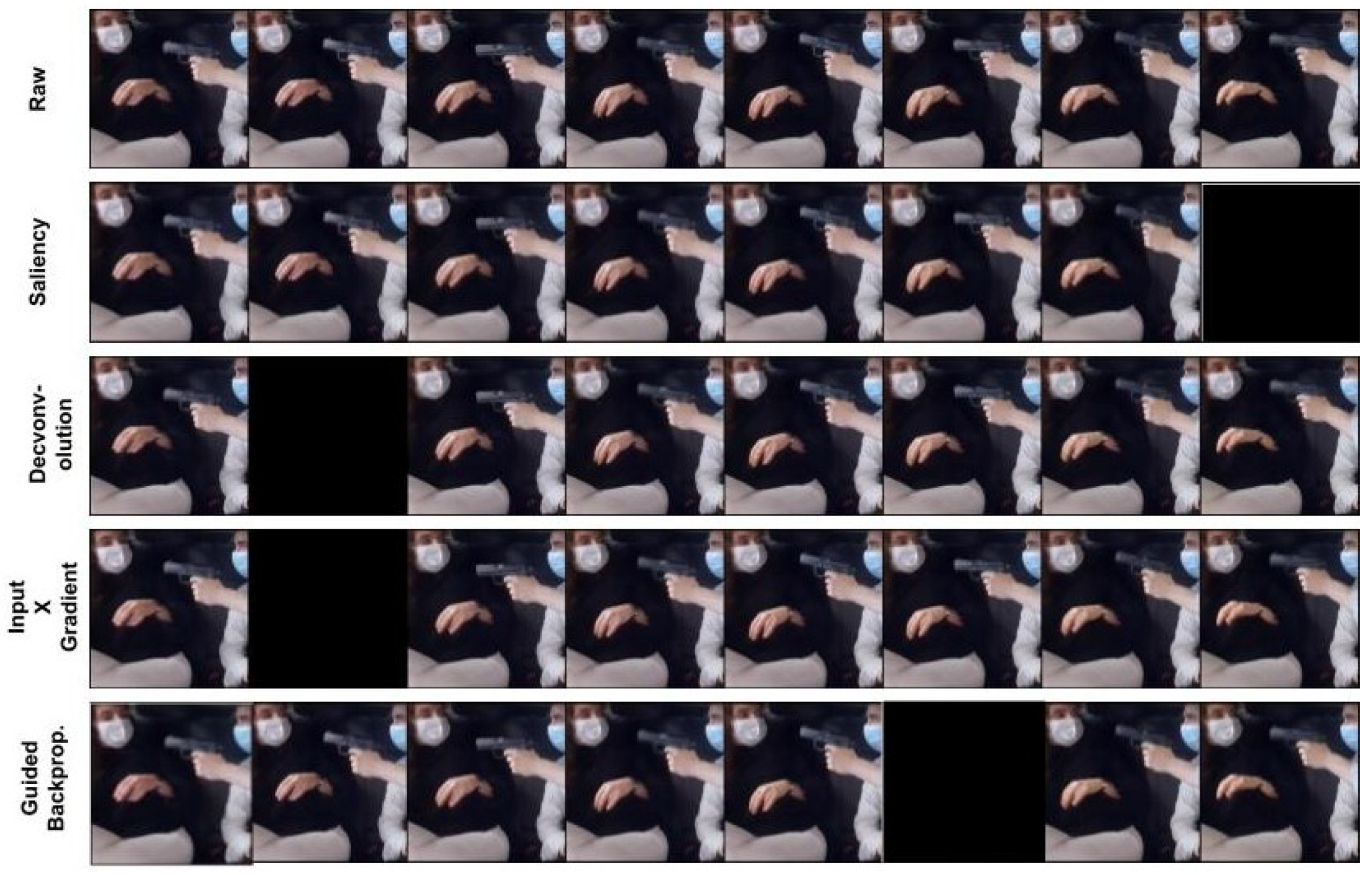
4.3.1. Temporal Analysis
Figure 5 shows how we perform the sanity-check of the temporal information. First we feed the model (
f) with the original video
v, then we obtain its prediction (
) and compute which frame is the most important to
. After obtaining the most important frame, we erased it information with 0 value yielding a new video
. Then, we fed the model with
to verify its new outputs
.
Table 4 present the temporal analysis on the test set and was constructed based on the three architectures model: X3D, C3D, and I3D. The baseline column raw is the f-measure presented in
Table 1. We have applied four different methods: Saliency, Deconvolution, InputxGradient, and Guided Backpropagation. We can observe that the X3D model presented better results on the four methods, thus being the most robust method in the temporal scenario. Still, I3D has also competitive results.
4.3.2. Spatial Analysis
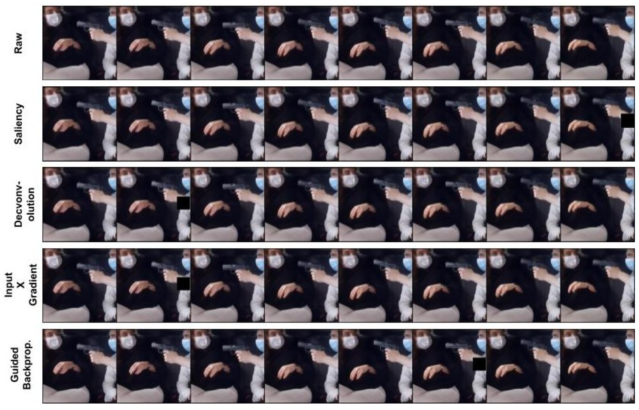
The spatial analysis is performed in a similar way as the temporal analysis. The difference is that we compute the most important subregion within the most crucial frame. The size of the subregion is a parameter to this analysis. In this experiment, we chose 40 × 40 as it is representative compared to the full size of each frame (224 × 224). In future work, we intended to analyse the impact of this parameter in the analysis.
Figure 6 shows an input sample about how we performed this analysis, besides
Table 5 presents the results obtained.
Table 5 presented the spatial analysis with the three architectures model: X3D, C3D, and I3D. It was also applied in the same way in four different methods: Saliency, Deconvolution, Input × Gradient, and Guided Backpropagation. We can observe that X3D and I3D models presented better results in four methods.
Based on the temporal and spatial analysis, we can observe that the two models, X3D and I3D, have better sanity-check results based on interpretability, thus showing that they are more robust than the C2D model.
In terms of qualitative analysis
Figure 6 shows an interesting phenomenon, it shows that the model is not using the correct information to perform its prediction, while an actor is using a weapon to threaten another actor, the model focuses on the actor’s hand instead of the violent object in the scene. This weakness is not restricted to in-car violence recognition models, and it is an active area of research in deep learning named Right for the right reasons [
37].
5. Conclusions
This paper presents three models for in-car violence recognition and evaluates these models based on adversarial attacks and interpretability methods. So, we begin to present adversarial attack and interpretability methods and architectures models. Then, we describe the dataset, beginning to explain the dataset recording, the violence and non-violent scenarios, the dataset pre-processing, and the final dataset used. In addition, we have presented the three prominent architectures used in the study. In the analysis, we have begun to analyse the model’s convergence, followed by adversarial robustness on video and frame level for each model. Finally, we analysed the sanity check based on interpretability, conducting temporal and spatial analysis.
The analysis shows that the I3D model is the most adversarial robust, while the X3D model presented better results in the original data distribution and the sanity checks. In addition, the qualitative discussion regarding the model interpretability shows that the models can be inferred correctly based on the wrong information. Thus, this work shows that although the in-car violence recognition models present good results in the test set, they still have room for improvement in their robustness. In future work, we intend to employ the right for the right reasons methods during the training to make the models infer correctly based on the right signal.
Author Contributions
Conceptualization by F.S., D.D. and F.S.M.; Supervision by N.H., J.M. and P.N. All authors have read and agreed to the published version of the manuscript.
Funding
This work is funded by “FCT—Fundação para a Ciência e Tecnologia” within the R&D Units Project Scope: UIDB/00319/2020. The employment contract of Dalila Durães is supported by CCDR-N Project: NORTE-01-0145-FEDER-000086.
Institutional Review Board Statement
Not applicable.
Informed Consent Statement
Not applicable.
Data Availability Statement
Data available on request due to restrictions eg privacy or ethical.
Conflicts of Interest
The authors declare no conflict of interest.
References
- Marcondes, F.S.; Durães, D.; Gonçalves, F.; Fonseca, J.; Machado, J.; Novais, P. In-vehicle violence detection in carpooling: A brief survey towards a general surveillance system. In International Symposium on Distributed Computing and Artificial Intelligence; Springer: Cham, Switzerland, 2020; pp. 211–220. [Google Scholar]
- Durães, D.; Marcondes, F.S.; Gonçalves, F.; Fonseca, J.; Machado, J.; Novais, P. Detection violent behaviors: A survey. In International Symposium on Ambient Intelligence; Springer: Cham, Switzerland, 2020; pp. 106–116. [Google Scholar]
- Jesus, T.; Duarte, J.; Ferreira, D.; Durães, D.; Marcondes, F.; Santos, F.; Gomes, M.; Novais, P.; Gonçalves, F.; Fonseca, J.; et al. Review of trends in automatic human activity recognition using synthetic audio-visual data. In International Conference on Intelligent Data Engineering and Automated Learning; Springer: Cham, Switzerland, 2020; pp. 549–560. [Google Scholar]
- Neves, J.; Machado, J.; Analide, C.; Novais, P.; Abelha, A. Extended logic programming applied to the specification of multi-agent systems and their computing environments. In Proceedings of the 1997 IEEE International Conference on Intelligent Processing Systems (Cat. No. 97TH8335), Beijing, China, 28–31 October 1997; Volume 1, pp. 159–164. [Google Scholar]
- Freitas, P.M.; Andrade, F.; Novais, P. Criminal liability of autonomous agents: From the unthinkable to the plausible. In International Workshop on AI Approaches to the Complexity of Legal Systems; Springer: Berlin/Heidelberg, Germany, 2013; pp. 145–156. [Google Scholar]
- Durães, D.; Bajo, J.; Novais, P. Characterize a human-robot interaction: Robot personal assistance. In Personal Assistants: Emerging Computational Technologies; Springer: Cham, Switzerland, 2018; pp. 135–147. [Google Scholar]
- Toala, R.; Durães, D.; Novais, P. Human-computer interaction in intelligent tutoring systems. In Proceedings of the International Symposium on Distributed Computing and Artificial Intelligence, Ávila, Spain, 26–28 June 2019; Springer: Cham, Switzerland, 2019; pp. 52–59. [Google Scholar]
- Xia, P.; Li, Z.; Niu, H.; Li, B. Understanding the Error in Evaluating Adversarial Robustness. arXiv 2021, arXiv:2101.02325. [Google Scholar]
- Szegedy, C.; Zaremba, W.; Sutskever, I.; Bruna, J.; Erhan, D.; Goodfellow, I.; Fergus, R. Intriguing properties of neural networks. arXiv 2013, arXiv:1312.6199. [Google Scholar]
- Santos, F.; Durães, D.; Marcondes, F.S.; Lange, S.; Machado, J.; Novais, P. Efficient Violence Detection Using Transfer Learning. In Practical Applications of Agents and Multi-Agent Systems; Springer: Cham, Switzerland, 2021; pp. 65–75. [Google Scholar]
- Feichtenhofer, C. X3d: Expanding architectures for efficient video recognition. In Proceedings of the IEEE/CVF Conference on Computer Vision and Pattern Recognition, Seattle, WA, USA, 13–19 June 2020; pp. 203–213. [Google Scholar]
- Cheng, M.; Cai, K.; Li, M. RWF-2000: An open large scale video database for violence detection. In Proceedings of the 2020 25th International Conference on Pattern Recognition (ICPR), Milan, Italy, 10–15 January 2021; pp. 4183–4190. [Google Scholar]
- Goodfellow, I.J.; Shlens, J.; Szegedy, C. Explaining and harnessing adversarial examples. arXiv 2014, arXiv:1412.6572. [Google Scholar]
- Madry, A.; Makelov, A.; Schmidt, L.; Tsipras, D.; Vladu, A. Towards deep learning models resistant to adversarial attacks. arXiv 2017, arXiv:1706.06083. [Google Scholar]
- Carlini, N.; Wagner, D. Towards evaluating the robustness of neural networks. In Proceedings of the 2017 IEEE Symposium on Security and Privacy (SP), San Jose, CA, USA, 22–26 May 2017; pp. 39–57. [Google Scholar]
- Dong, S.; Wang, P.; Abbas, K. A survey on deep learning and its applications. Comput. Sci. Rev. 2021, 40, 100379. [Google Scholar] [CrossRef]
- Wong, E.; Rice, L.; Kolter, J.Z. Fast is better than free: Revisiting adversarial training. In Proceedings of the 8th International Conference on Learning Representations, ICLR 2020, Addis Ababa, Ethiopia, 26–30 April 2020. [Google Scholar]
- Inkawhich, N.; Inkawhich, M.; Chen, Y.; Li, H. Adversarial attacks for optical flow-based action recognition classifiers. arXiv 2018, arXiv:1811.11875. [Google Scholar]
- Zuo, C. Regularization effect of fast gradient sign method and its generalization. arXiv 2018, arXiv:1810.11711. [Google Scholar]
- Tramèr, F.; Kurakin, A.; Papernot, N.; Goodfellow, I.J.; Boneh, D.; McDaniel, P.D. Ensemble Adversarial Training: Attacks and Defenses. In Proceedings of the 6th International Conference on Learning Representations, ICLR 2018, Vancouver, BC, Canada, 30 April–3 May 2018. [Google Scholar]
- Kurakin, A.; Goodfellow, I.J.; Bengio, S. Adversarial Machine Learning at Scale. In Proceedings of the 5th International Conference on Learning Representations, ICLR 2017, Toulon, France, 24–26 April 2017. [Google Scholar]
- Shafahi, A.; Najibi, M.; Ghiasi, A.; Xu, Z.; Dickerson, J.P.; Studer, C.; Davis, L.S.; Taylor, G.; Goldstein, T. Adversarial training for free! In Proceedings of the Advances in Neural Information Processing Systems 32: Annual Conference on Neural Information Processing Systems 2019, NeurIPS 2019, Vancouver, BC, Canada, 8–14 December 2019; pp. 3353–3364. [Google Scholar]
- Zeiler, M.D.; Fergus, R. Visualizing and understanding convolutional networks. In European Conference on Computer Vision; Springer: Cham, Switzerland, 2014; pp. 818–833. [Google Scholar]
- Simon, M.; Rodner, E.; Denzler, J. Part detector discovery in deep convolutional neural networks. In Asian Conference on Computer Vision; Springer: Cham, Switzerland, 2014; pp. 162–177. [Google Scholar]
- Simonyan, K.; Vedaldi, A.; Zisserman, A. Deep Inside Convolutional Networks: Visualising Image Classification Models and Saliency Maps. In Proceedings of the 2nd International Conference on Learning Representations, ICLR 2014, Banff, AB, Canada, 14–16 April 2014. [Google Scholar]
- Springenberg, J.T.; Dosovitskiy, A.; Brox, T.; Riedmiller, M.A. Striving for Simplicity: The All Convolutional Net. In Proceedings of the 3rd International Conference on Learning Representations, ICLR 2015, San Diego, CA, USA, 7–9 May 2015. [Google Scholar]
- Selvaraju, R.R.; Cogswell, M.; Das, A.; Vedantam, R.; Parikh, D.; Batra, D. Grad-cam: Visual explanations from deep networks via gradient-based localization. In Proceedings of the IEEE International Conference on Computer Vision, Venice, Italy, 22–29 October 2017; pp. 618–626. [Google Scholar]
- Sundararajan, M.; Taly, A.; Yan, Q. Axiomatic Attribution for Deep Networks. In Proceedings of the 34th International Conference on Machine Learning, ICML 2017, Sydney, Australia, 6–11 August 2017; Volume 70, pp. 3319–3328. [Google Scholar]
- Xu, S.; Venugopalan, S.; Sundararajan, M. Attribution in Scale and Space. In Proceedings of the 2020 IEEE/CVF Conference on Computer Vision and Pattern Recognition, CVPR 2020, Seattle, WA, USA, 13–19 June 2020; pp. 9677–9686. [Google Scholar] [CrossRef]
- Shrikumar, A.; Greenside, P.; Kundaje, A. Learning Important Features Through Propagating Activation Differences. In Proceedings of the 34th International Conference on Machine Learning, ICML 2017, Sydney, Australia, 6–11 August 2017; Volume 70, pp. 3145–3153. [Google Scholar]
- Lundberg, S.M.; Lee, S. A Unified Approach to Interpreting Model Predictions. In Proceedings of the Advances in Neural Information Processing Systems 30: Annual Conference on Neural Information Processing Systems 2017, Long Beach, CA, USA, 4–9 December 2017; pp. 4765–4774. [Google Scholar]
- Albawi, S.; Bayat, O.; Al-Azawi, S.; Ucan, O.N. Social touch gesture recognition using convolutional neural network. Comput. Intell. Neurosci. 2018, 2018, 6973103. [Google Scholar] [CrossRef] [PubMed] [Green Version]
- Carreira, J.; Zisserman, A. Quo vadis, action recognition? A new model and the kinetics dataset. In Proceedings of the IEEE Conference on Computer Vision and Pattern Recognition, Honolulu, HI, USA, 21–26 July 2017; pp. 6299–6308. [Google Scholar]
- Huang, G.; Liu, Z.; Van Der Maaten, L.; Weinberger, K.Q. Densely connected convolutional networks. In Proceedings of the IEEE Conference on Computer Vision and Pattern Recognition, Honolulu, HI, USA, 21–26 July 2017; pp. 4700–4708. [Google Scholar]
- Durães, D.; Santos, F.; Marcondes, F.S.; Machado, J.; Novais, P. In-Car: Video Violence Recognition Dataset. University of Minho, Braga, Portugal. 2022; unpublished manuscript. [Google Scholar]
- Arthur Oliveira Santos, F.; Zanchettin, C.; Nogueira Matos, L.; Novais, P. On the Impact of Interpretability Methods in Active Image Augmentation Method. Log. J. IGPL 2021. [Google Scholar] [CrossRef]
- Shao, X.; Skryagin, A.; Stammer, W.; Schramowski, P.; Kersting, K. Right for Better Reasons: Training Differentiable Models by Constraining their Influence Functions. In Proceedings of the Thirty-Fifth AAAI Conference on Artificial Intelligence, AAAI 2021 and Thirty-Third Conference on Innovative Applications of Artificial Intelligence, IAAI 2021 and the Eleventh Symposium on Educational Advances in Artificial Intelligence, EAAI 2021, Virtual Event, 2–9 February 2021; pp. 9533–9540. [Google Scholar]
Figure 1.
Visualizing the model convergence by computing the training loss for each epoch. The x-axis represents the epoch and the y-axis represents the respective cross-entropy training loss.
Figure 1.
Visualizing the model convergence by computing the training loss for each epoch. The x-axis represents the epoch and the y-axis represents the respective cross-entropy training loss.
Figure 2.
Visualizing the model convergence by computing the training accuracy for each epoch. The x-axis represents the epoch and the y-axis represents the respective training accuracy.
Figure 2.
Visualizing the model convergence by computing the training accuracy for each epoch. The x-axis represents the epoch and the y-axis represents the respective training accuracy.
Figure 3.
Video level adversarial attack. In this figure, we show how we can obtain the video level adversarial attack. (a) Shows a sequence of the input frames, (b) presents the adversarial noise obtained from the FGSM, and (c) shows the complete video adversarial attack resultant after add adversarial noise on each input frame.
Figure 4.
Frame-level adversarial attack. This example shows how we can compute the frame-level adversarial attack. The (a) represents the input video, (b) the frame adversarial noise, and (c) the frame-level adversarial attack. In this example, we only add adversarial noise on the fifth frame.
Figure 4.
Frame-level adversarial attack. This example shows how we can compute the frame-level adversarial attack. The (a) represents the input video, (b) the frame adversarial noise, and (c) the frame-level adversarial attack. In this example, we only add adversarial noise on the fifth frame.
Figure 5.
Temporal analysis. This example shows an example of the temporal analysis. Each row show the frame occlude though each interpretability method used.
Figure 5.
Temporal analysis. This example shows an example of the temporal analysis. Each row show the frame occlude though each interpretability method used.
Figure 6.
Spatial analysis. This example shows an example of the spatial analysis. Each row show the subregion occlude though each interpretability method used.
Figure 6.
Spatial analysis. This example shows an example of the spatial analysis. Each row show the subregion occlude though each interpretability method used.
Table 1.
Results on the test set. This table presents the f-measure value for each model evaluated in the test set. The column architecture represent the model evaluated while the f-measure represents the results obtained.
Table 1.
Results on the test set. This table presents the f-measure value for each model evaluated in the test set. The column architecture represent the model evaluated while the f-measure represents the results obtained.
| Architecture | F-Measure | Data Split |
|---|
| X3D | 78, 02 | Test |
| C2D | 65, 44 | Test |
| I3D | 72, 36 | Test |
Table 2.
Video-level results. The column metric means which one was used to compute the result and the adversarial attack column means which method was used to compute the attack. Each row represents an experimentation scenario.
Table 2.
Video-level results. The column metric means which one was used to compute the result and the adversarial attack column means which method was used to compute the attack. Each row represents an experimentation scenario.
| Architecture | Metric | Value | Adversarial Attack |
|---|
| X3D | F1 | 0, 0 | FGSM |
| X3D | F1 | 0, 0 | PGD |
| C2D | F1 | 3, 86 | FGSM |
| C2D | F1 | 4, 89 | PGD |
| I3D | F1 | 45, 89 | FGSM |
| I3D | F1 | 0, 0 | PGD |
| X3D | Accuracy | 0, 0 | FGSM |
| X3D | Accuracy | 0, 0 | PGD |
| C2D | Accuracy | 22, 73 | FGSM |
| C2D | Accuracy | 0, 0 | PGD |
| I3D | Accuracy | 35, 40 | FGSM |
| I3D | Accuracy | 9, 56 | PGD |
Table 3.
Frame-level results. This table presents the f-measure value for each model evaluated in the test set. The column architecture represent the model evaluated while the value represents the f-measure results obtained.
Table 3.
Frame-level results. This table presents the f-measure value for each model evaluated in the test set. The column architecture represent the model evaluated while the value represents the f-measure results obtained.
| Architecture | Metric | Value | Frame | Adversarial Attack |
|---|
| X3D | F1 | 64, 04 | 4 | FGSM |
| X3D | F1 | 53, 97 | 4 | PGD |
| X3D | F1 | 65, 04 | 9 | FGSM |
| X3D | F1 | 56, 85 | 9 | PGD |
| C2D | F1 | 33, 86 | 3 | FGSM |
| C2D | F1 | 29, 13 | 3 | PGD |
| C2D | F1 | 28, 81 | 6 | FGSM |
| C2D | F1 | 26, 72 | 6 | PGD |
| I3D | F1 | 66, 66 | 3 | FGSM |
| I3D | F1 | 62, 91 | 3 | PGD |
| I3D | F1 | 65, 80 | 6 | FGSM |
| I3D | F1 | 62, 87 | 6 | PGD |
Table 4.
Results of the temporal analysis on the test set. This table presents the f-measure value for each model evaluated in the test set based on the sanity-check analysis. The column architecture represent the model evaluated while the saliency, deconvolution, input × gradient, and guided backpropagation represents the results obtained from the sanity check with the respective interpretability method. The column raw is the baseline results.
| Architecture | Raw | Saliency | Deconvolution | Input × Gradient | Guided Backpropagation |
|---|
| X3D | 78, 02 | 56, 14 | 52, 29 | 51, 28 | 50, 85 |
| C2D | 65, 44 | 44, 07 | 26, 66 | 23, 58 | 23, 41 |
| I3D | 72, 36 | 52, 29 | 52, 10 | 51, 29 | 50, 29 |
Table 5.
Results of the spatial analysis on the test set. As in
Table 4, this table presents the f-measure value for each model evaluated in the test set based on the sanity-check analysis. The meaning of each column is the same as in
Table 4, except that here is the spatial sanity check.
Table 5.
Results of the spatial analysis on the test set. As in
Table 4, this table presents the f-measure value for each model evaluated in the test set based on the sanity-check analysis. The meaning of each column is the same as in
Table 4, except that here is the spatial sanity check.
| Architecture | Raw | Saliency | Deconvolution | Input × Gradient | Guided Backpropagation |
|---|
| X3D | 78, 02 | 77, 84 | 52, 29 | 52, 20 | 52, 10 |
| C2D | 65, 44 | 33, 88 | 06, 21 | 11, 98 | 08, 48 |
| I3D | 72, 36 | 60, 07 | 52, 29 | 52, 05 | 51, 79 |
| Publisher’s Note: MDPI stays neutral with regard to jurisdictional claims in published maps and institutional affiliations. |
© 2022 by the authors. Licensee MDPI, Basel, Switzerland. This article is an open access article distributed under the terms and conditions of the Creative Commons Attribution (CC BY) license (https://creativecommons.org/licenses/by/4.0/).


 ,
, 


