Abstract
A particular 1D II-order differential semi-linear elliptic model for electrostatic membrane MEMS devices, which is well-known in the literature, considers the amplitude of the electric field locally proportional to the membrane’s geometric curvature, which contains a term involving the fringing field according to Pelesko and Driscoll’s theory. Thus, in this paper, we will begin from this elliptical model, of which the uniqueness condition for the solution does not depend on the electromechanical properties of the membrane’s constituent material. In particular, after analyzing the model’s advantages and disadvantages, we present a new uniqueness condition for the solution depending on the properties listed above, which appears to be more important than the existence condition of the solution that is well-known in literature. Therefore, once the fringing field’s mode of action on the electrostatic force acting on the membrane is evaluated, suitable numerical techniques are used and compared to recover the membrane profile without ghost solutions and to propose an innovative criterion for selecting the membrane material, which depends on the electrical operative parameters and vice-versa. Finally, the possible industrial uses of the studied device are evaluated.
1. Introduction to The Problem
Recently, the industrial-scale production of electromechanical components has required the increasingly intense development of devices at highly competitive costs, combining the physics of the problem with low-level machine languages [1,2,3]. Among these devices, it is imperative to include microbeams, microresonators and electrostatic MEMS devices [4,5,6], as today’s engineering is increasingly oriented towards the design and manufacture of miniaturized devices [7,8,9,10]. Furthermore, modern technologies allow the prototyping, production and marketing of special MEMS devices such as circular graphene-membrane MEMS systems [11,12], SiN circular-membrane MEMS systems [13,14] and the most sophisticated CMOS MEMS-based membrane-bridges [15]. However, even though these devices are industrially quite simple to produce [1,2,16], they are often supported by extremely complex physical-mathematical modeling that hardly provides solutions (usually, the profile of the deforming element, , ) in explicit form due to the strong non-linearities (and/or singularities) in the mathematical models [17,18,19]. Even though it requires demanding studies, this kind of MEMS modeling is very useful because it allows one to evaluate the mechanical stress states of all those elements that, internally, are responsible for movement in relation to particular uses of the device [19]. Furthermore, the modeling enables prediction tests of the device’s functionality without performing them on the real device which, often, would lead to the destruction of the device itself [20]. So, in these cases, to recover the profile of the deforming element, it is imperative to use specific numerical techniques to achieve solutions that, if they do not respect the analytical conditions of existence and/or uniqueness, represent ghost solutions [19,21,22]. The problem of ghost solutions has proved to be crucial, especially for MEMS membrane devices of which the amplitude of the electric field, , has proved to be locally proportional to the curvature of the membrane, generating interesting second-order semi-linear differential models with Dirichlet boundary conditions of which the existence and uniqueness conditions do not depend, at least explicitly, on the electromechanical properties of the material constituting the membrane (see [19,21] and references therein). Furthermore, this type of micro-device suffers from the effects of the fringing field phenomenon (frequently observed in industrial MEMS devices when both the length and height of the device are of orders of comparable magnitude), comprising the bending of the lines of force of at the edges of the device, which could influence the deformation of the deformable element, even touching the upper plate, and thereby generating an unwanted and simultaneously dangerous electrostatic discharge. Particularly, as one moves away from the edges, the curvature of the lines of force of decrease until it becomes zero at the central area of the device. Highlighting that there is no trace of terms taking into account the effects caused by the fringing field in the models studied in [19,21,23,24,25], the following 1D second-order differential semi-linear elliptic model with homogeneous boundary conditions has been studied according to the Pelesko–Driscoll theory [26]:
in which is locally proportional to the curvature of the membrane and is the critical security distance ensuring that the membrane does not touch the top of the device, avoiding undesirable electrostatic discharges. Moreover, , with the ′ first derivative with respect to x, considers the effect due to the fringing field in which , a real positive number, weighs the effect due to the fringing field. Obviously, (1) does not provide explicit solutions (see [23]). Therefore, a useful algebraic condition ensuring that the solutions depend on the membrane material’s electromechanical properties must be obtained. Furthermore, we also note that, in [23], the uniqueness condition for the solution of the model (1) does not depend on the membrane’s properties. Thus, the main purposes of this paper can be summarized in the following items:
- To evaluate how the effect due to the fringing field affects the electrostatic force in the device, obtaining an increase for the total electrostatic force ;
- To achieve a new uniqueness condition of the solution for (1), which depends on the electromechanical properties of the membrane and the real parameter that weights the effects due to the fringing field;
- Starting from the uniqueness condition obtained in the previous item, obtaining a new, unique condition ensuring both existence and uniqueness for (1), which depend on both the electromechanical properties of the membrane and the real parameter that weights the effects due to the fringing field;
- To recover the membrane profile by means of numerical techniques consolidated in the literature, which represent the most suitable techniques for the numerical solution of second-order elliptic semi-linear differential models. These techniques (based on shooting procedures, Keller box schemes and Lobatto formulas) have been implemented in MatLab® R2019a running on an Intel Core 2 CPU at 1.45 GHz, comparing their performances as real parameters that weight the effect due to the varying fringing field, in order to achieve suitable ranges for the membrane material’s electromechanical properties that ensure convergence (even with ghost solutions); and
- Finally, to obtain the important link between the mechanical properties of the material constituting the membrane and the electrical operating parameters of the device without ghost solutions (which is interesting for industrial applications).
The remainder of the paper is organized as follows. Section 2 briefly describes the 1D electrostatic membrane MEMS considered in our study from the point of view of the actuator and that of the sensor, whereas Section 3 details the mathematical model governing the behavior of the device. Some advantages and disadvantages of the model are discussed in Section 4, whereas Section 5 and Section 6 detail a well-known result on the existence of at least one solution of the model under study and a new algebraic condition ensuring the uniqueness of the solution, respectively. In the following, Section 7 and Section 8 discuss a new algebraic condition ensuring both existence and uniquenes and how the fringing field affects the electrostatic force in the device, respectively. The exploited numerical techniques are presented in Section 9, whereas the most important numerical results are presented and discussed in Section 10. Two important limitations for the mechanical tension of the membrane and the external voltage are discussed in Section 11, and Section 12 points out the influence of electromechanical properties on the proposed procedure. Finally, the destinations of use of the device are discussed in Section 13. Some conclusions and perspectives end the paper. As regards the units of measurement of each physical quantity involved, please refer to the Abbreviations at the end of the paper.
2. A Brief Description of the 1D Electrostatic MEMS Device
2.1. The Device Functioning as an Actuator
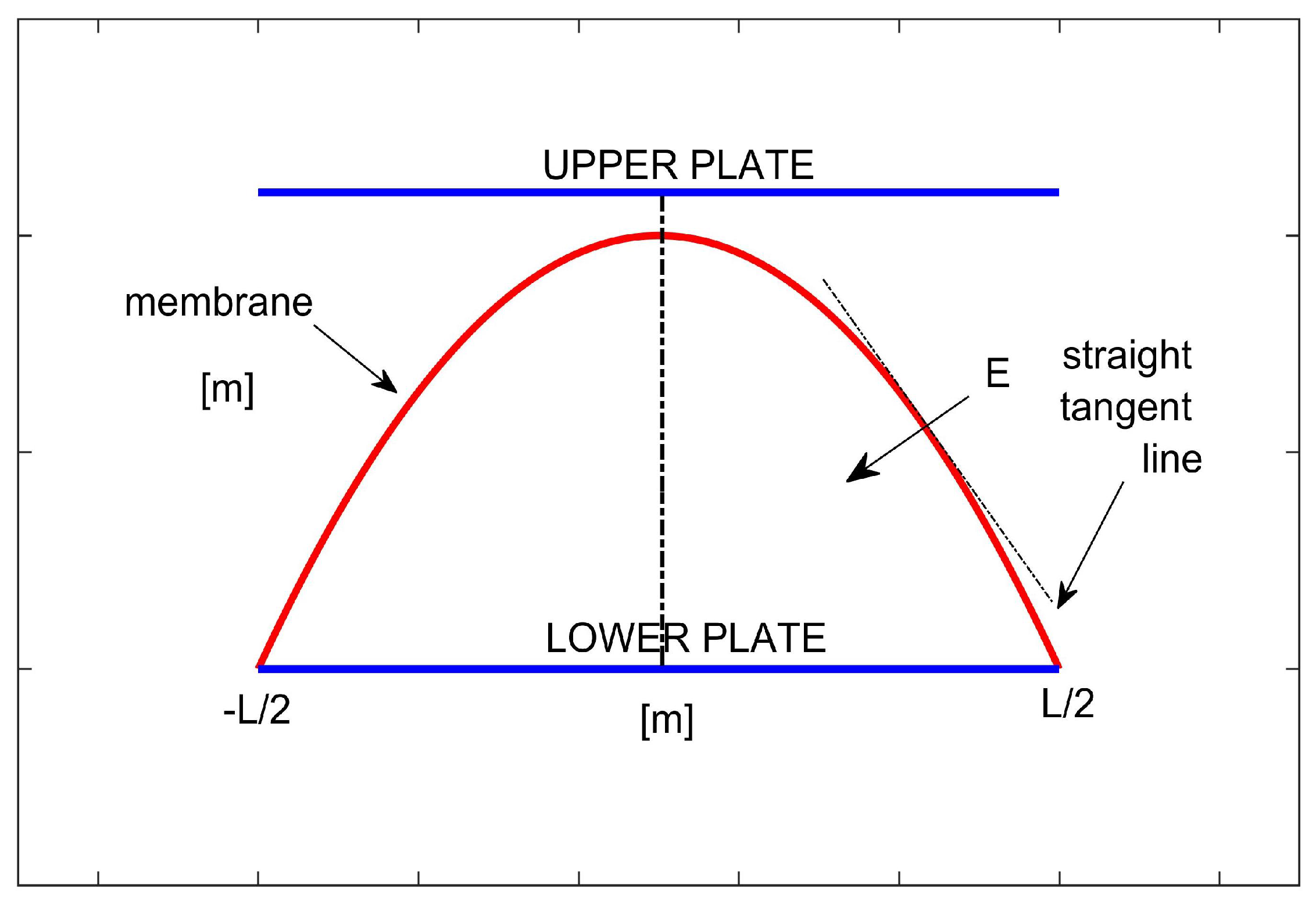
In we consider a system of orthonormal Cartesian axes , in which y identifies the vertical axis. As shown in Figure 1, the device is composed of two parallel plates (of the same metal) placed at the distance d from each other, whereas the length of the plates is indicated by L. For computational purposes only, we place the device so that the y axis is also the axis of symmetry for the device, whereas the x axis is the straight line of the lower plate. On the latter, acting as a support, there is a membrane (of which the material has certain electromechanical properties) but at its edges to the edges of the lower plate it deforms when an external electric voltage, V, is applied between the two plates. By applying V, the upper plate assumes the electrostatic potential V, whereas the lower plate is at , so that the membrane deforms towards the upper plate without touching it (to avoid unwanted electrostatic discharges). Therefore, the membrane profile, u, becomes a function of x (i.e., ).
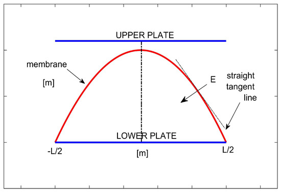
Figure 1.
Schematic of the 1D membrane MEMS device studied. The parallel metallic plates are represented in blue, whereas the membrane is indicated in red. The orthogonality between and the tangent line to the membrane are also highlighted.
Remark 1.
The membrane, although made of a light material, has a certain mechanical inertia which is overcome if V generates a value of in the device capable of producing electrostatic pressure, , which is able to supercede the aforementioned inertia. As noted in other works [1], if is the permittivity of the free space,
so that the electrostatic force acting on the membrane, , considering that locally
becomes
deflects the membrane towards the upper plate, achieving a displacement at , , computable as [1,23]
where T is the mechanical tension of the membrane when it is at rest.
Remark 2.
(5) is a rudimentary approach to device control. In fact, once T has been fixed (i.e., the material constituting the membrane has been chosen), it is possible, based on (5), to select V so that . Then,
So, V cannot exceed the computable value from the right side of (6). It is worth noting that the ratio plays a major role in the V limitation. Moreover, if , the effect due to the fringing field must be considered [23,26].
2.2. The Device Functioning as a Sensor
To understand the deformation mechanisms of a membrane, we start by considering a metal plate subjected to a mechanical pressure p, of which the deflection, u, satisfies the following hyperbolic PDE [1,19]:
where is the density of the plate, h is its thickness, and D is the stiffness coefficient of the material constituting the plate. As known, in steady-state conditions,
which can be written as . Here, the device acts as a transducer because p deforms the plate. Moreover, being both D and h-bounded values, it follows that the distance between the plates remains almost constant (i.e., almost equal to d and ). Therefore, the electrostatic capacitance of the device, , depends on , as proven in [19,23]. Moreover, by means of the Taylor series and for , it is easy to write at equilibrium. Finally, it is also possible to achieve [19,23].
A different situation occurs when considering an MEMS membrane device. In this case, h is certainly negligible, so due to the continuum mechanics D is also negligible. Therefore, grows with an evidently increased risk that the membrane will touch the upper plate [19,23]. In this case, it is easy to observe that
Finally, concerning , (4) is still valid.
Remark 3.
and assume that the membrane is at rest. This hypothesis is fully justified because, for the most common membrane MEMS devices, . It follows that the surface value of the deformed membrane is almost equal to the surface value of the membrane at rest, as though, with reference to the membrane, the regime of small displacements were established.
There is also an interesting link between p and , which was studied in [23]. In fact, since according to (9) , with , and considering that p is proportional to , it follows that
3. The Mathematical Model Governing the Behavior of the Device
3.1. From the Electrostatic MEMS Device with Two Parallel Metallic Plates to the 1D Electrostatic Membrane MEMS Device
As shown in [1], the most accredited model for industrial electrostatic membrane MEMS devices is derived from the following IV-order differential dimensionless model with Dirichlet conditions, concerning two parallel metallic-plate electrostatic MEMS devices (with equal and finite thickness) in which the ground plate deforms towards the upper one:
In (11), is the unknown profile of the deflecting plate; ; represents the stretching energy of the deformable plate and is its stretching parameter; represents a bounded function that carries the dielectric properties of the material constituting the deflecting plate; is a parameter depending on the electrostatic capacitance, , of the device’s control circuit’s capacitor; is the drop voltage between the plates, computable as [1,23]
which represents the tuning parameter of the device (because it is directly linked to V), so that
represents the electrostatic load function.
Remark 4.
We note that . In fact, if bifurcation phenomena could occur [1], which, as is known, could cause instability of the membrane, leading to its rupture in extreme cases.
Remark 5.
locally establishes the type of stress on the membrane when external V is applied. Particularly, V determines in the device, which locally generates and, consequently, acts on the membrane, which deforms towards the upper plate, avoiding contact between them. Then, must be strictly correlated with V (to control the device in terms of voltage) as well as the dielectric, mechanical, and geometric properties of the membrane.
In this work, we consider a 1D membrane MEMS device, so that based on (11), for a membrane , it follows that ; thus, . Moreover, given that the membrane’s contributions due to stretching are to be considered negligible, it follows that and (see [1]) . The capacitive term can be considered negligible (); therefore, . Finally, is constant and assumes a unitary value. Therefore, taking into account that in 1D geometry , (11) becomes [23,27]:
which represents the 1D dimensionless model for our membrane MEMS device, as depicted in Figure 1.
3.2. The Fringing Field Problem and the Pelesko–Driscoll Theory
A membrane MEMS device can be considered a capacitor since it is formed of a pair of parallel metal plates (the deformable membrane is mounted on one of them) to which an external V is applied, causing an between them (the air between the plates acts as a dielectric). exists not only directly between the plates (conductive elements), but extends over a certain distance. This phenomenon is known as a fringing field, which is manifested by the bending of the electric flow lines towards the edge of the device, creating real fringes. On the inside (i.e., moving away from the edges), the flow lines are homogeneous and parallel. As is known, these effects are strictly related to the dimensions of the device [19,23,26]. Particularly, if d L, effects due to the fringing field appear and, according to the Pelesko–Driscoll theory [26], they can be modeled by means of an additive term written as
in which is an “ad hoc” bounded function describing these effects as we get closer to the edges of the device. As we approach the center, it significantly attenuates until it disappears at the center. Pelesko and Driskoll proved that (15) assumes the following form:
which, in our case, becomes
where is a real parameter that weights the effects due to the fringing field. Therefore, according to this theory, model (14) becomes
and exploiting (17), we can write the following II-order semi-linear elliptic model as follows:
3.3. On the Local Proportionality between and the Curvature of the Membrane
As specified in (13),
represents the electrostatic load function. Moreover, as it is dimensionless, it was proven that [19,23]
so that
Electrostatically, on the membrane is locally orthogonal to the straight tangent to the membrane (see Figure 1) [28] and was shown to be locally proportional to the extrinsic curvature of the membrane, , so that the following expression makes sense [19,23]:
where represents the function of proportionality, computed as [19,23]
Therefore, exploiting the usual 1D formulation of ,
we achieve the following 1D II-order differential semi-linear elliptic model with homogeneous boundary conditions [23]:
Remark 7.
In (27), it is imperative that . In fact, if , it would follow that , from which , where a and b are constant. Moreover, , physically, means that . In other words, would produce a linear deflection of the membrane when in the device (a physically impossible condition).
Remark 8.
The model, although it details many physical-mathematical aspects, does not consider further nonlinear phenomena (bifurcations, localized and/or distributed mechanical stresses, etc.). It follows that the study of (14) automatically introduces uncertainties which, at present, are not easily quantifiable.
3.4. On Possible Limitations for , , and
From (12) we deduce that when a particular device is chosen (that is, the value of T is selected) is proportional to . Thus, is limited by V. In other words, once a particular device is chosen, depends on its intended use. Vice versa, having chosen the intended use of the device (i.e., selected the value of V), it is the type of membrane (i.e., T) that limits the value of .
As proven in [19], has no limitations except that, of course, it must be non-null. What must catch our attention is the product . In fact, it will be subject to particular limitations due to problems concerning the convergence of the numerical techniques used for the recovery of the membrane profile.
As far as the function is concerned, during our study no apparent limitations to the attributable values emerged. However, mathematically, it is necessary that
in order to ensure that the membrane, locally, does not show tears.
Remark 9.
The most realistic MEMS models possess extremely complex physico-mathematical structures that are poorly suited to direct analytical studies. Therefore, they require simplifications, which almost always arise from simplifications of the device geometries. It follows that the results obtained from the study of the model are not reconciled with any experimental data obtainable directly in the laboratory. However, it is still worth studying the model as it provides a significant qualitative contribution to the study of the behavior of the device even if it is characterized by a somewhat simplified geometry.
4. Some Advantages and Disadvantages of the Model
The model has the main advantage of considering some physical phenomena that occur inside the device once the external V is applied. It considers the effects due to the fringing field by means of the addend dependent on , which is easily implementable in both software and hardware and controllable by V, given the presence of . Industrially, the membranes inside the device can be subject to possible “fatigue phenomena” caused by prolonged and continuous use. However, imposing that belongs to translates into admitting that, locally, the membrane does not allow excessive deformations (or even tears). The dielectric properties of the membrane material, as already mentioned, are represented by which, besides being limited for physical reasons, appears in the capacitive term of the model in which these properties are actually involved.
As already seen, is controllable by V. , in the model, is not controllable, so the effects due to the fringing field cannot be controlled in voltage. In addition, the model is statically formulated and does not have dynamic terms. Therefore, it is not possible to obtain (t, time variable), which is particularly useful for transitional studies.
Finally, the model does not allow one to obtain explicitly. Therefore, as a first approach, it is necessary to obtain conditions that ensure both the existence and the uniqueness of the solution. These conditions must be satisfied by the approximate solutions obtained through the use of suitable numerical techniques so as not to represent ghost solutions.
5. On the Existence of At Least One Solution: A Well Known Result
As proven in [23], the model admits an interesting algebraic condition of existence depending on both (the electromechanical parameters of the material constituting the membrane) and (the parameter that weights the effects due to the fringing field). For simpler reading, we report this critical result of existence in Proposition 1.
Proposition 1.
Remark 10.
As we will see below, condition (29) is less stringent than the condition that ensures uniqueness for the model (see Proposition 3). However, as proven in [19,23], (29) provides the following limitation for δ:
Obviously, can be excluded because it formalizes the absence of effects due to fringing fields. Furthermore, must be mathematically discarded. It is worth noting that in (29), physically, means that . Given that the deformed membrane in the device assumes a symmetrical position with respect to the axis of symmetry of the device itself, as we will see below, it makes sense that . However, consider that at , which means that the membrane, near the edges of the device, adheres to the lateral surface of the device, generating an unwanted and, at the same time, dangerous effect as it could create tears in the membrane itself during deformation.
Remark 11.
Equation (29) should be studied both as a function of the variation of δ and the electrical conductivity of the material constituting the membrane, depending on the temperature. This would certainly help us to understand if the device under study presents any bifurcation phenomena. However, in this work, we have limited ourselves to obtaining a limitation for δ, postponing more detailed results concerning the bifurcation phenomena to future works.
Remark 12.

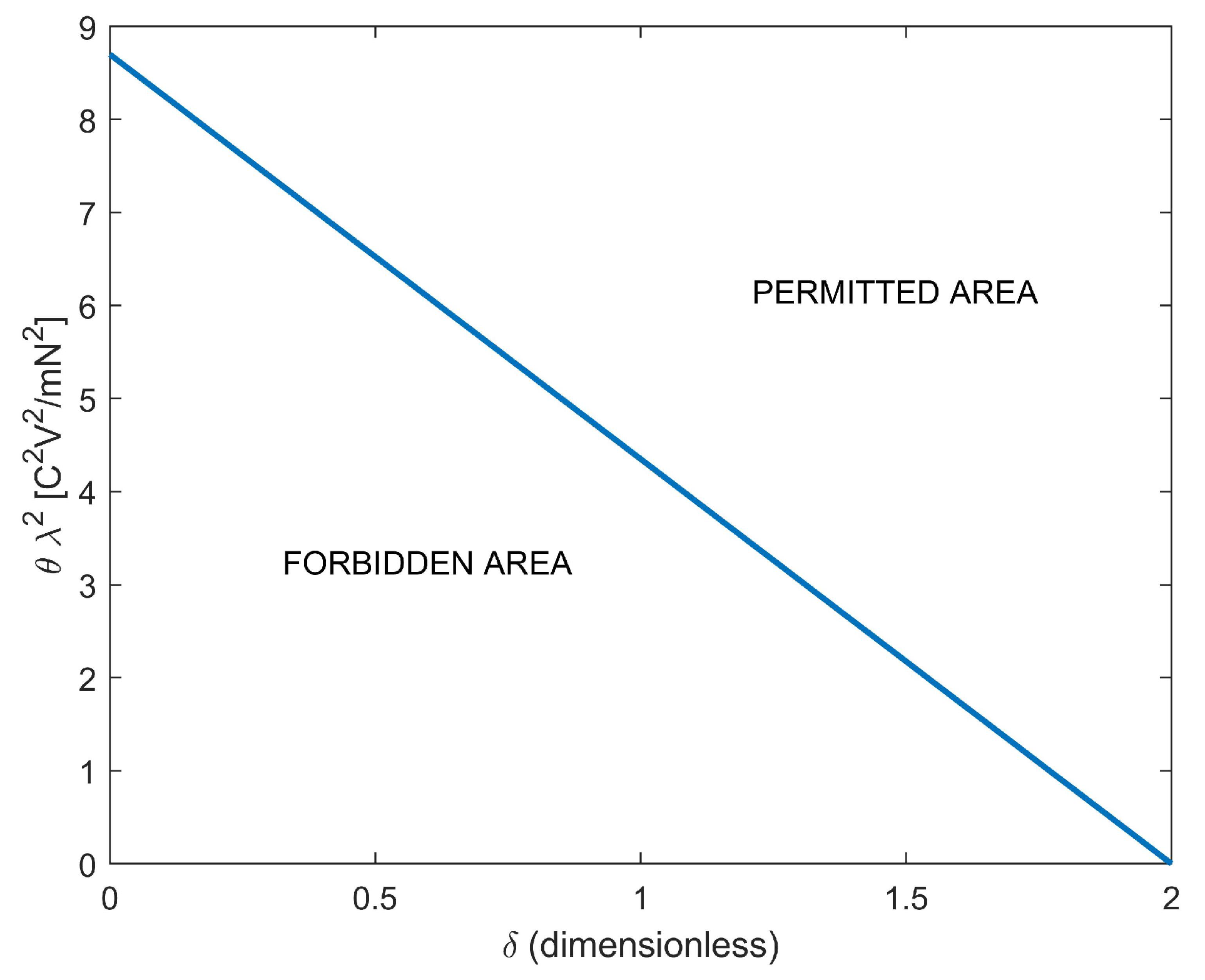
Condition (29) offers a useful link between and δ. Indeed, considering that, in dimensionless conditions, , and, from [23], , we easily achieve:
This means that as the fringing field effects increase, the separation between the allowed area and the forbidden area for is a straight line, as shown in Figure 2.
Figure 2.
A graphical representation of (31) when changes. The figure shows the forbidden area and that allowed as regards the values of .
Remark 13.
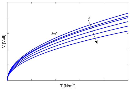
Taking into account condition (12), on the basis of (31), we can write:
which represents the link between V and T, depicted in Figure 3, when δ varies in its ranges (see (30)). Furthermore, we note that as δ increases, the curve tends to flatten (see Figure 3). In other words, when the effects due to the fringing field are substantial, the mechanical tension of the membrane can assume significant values even when the applied external V is extremely low. Finally, we note that it seems reasonable to think that θ is a very large positive real value, in order that V in (32) drops to acceptable values for the most common industrial applications. In fact, with , and taking into account (24), we can state
from which
Figure 3.
A graphical representation of (32) when changes.
In the usual industrial applications, , so that . Thus, θ increases enormously. Therefore, (32) makes sense.
6. A New Algebraic Condition Ensuring the Uniqueness of the Solution
As already mentioned, we present here a result of the solution’s uniqueness for the model, formalized by Proposition 2, dependent on both and .
Proposition 2.
Proof.
Model (1), exploiting a particular Green function, , can be formulated in its integral form [29]:
where [29]
and
has interesting properties that are useful for our purposes. Particularly,
- If ,otherwise, if
Let us consider two solutions, and , for model (1). Therefore, in ,
We observe that, for our purposes, is an adequate functional space, because we need to ensure that the membrane does not undergo excessive tearing or deformation during its motion towards the upper plate. Mathematically, this is guaranteed by the continuity of both and .
Therefore, exploiting (36), we can state:
Analogously,
Thus, (45) becomes
Exploiting well-known properties of the integrals, (48) becomes:
However, in [19], it was proven that
from which
Considering that
(52) becomes:
from which
and supposing that , , it follows from which
moreover, from (53), it follows that
so that (55) can be written as
Finally, to achieve a contradiction, we need to impose that
from which
If, absurdly,
it follows that
which represents a physically untrue condition (just substitute the usual numerical values for each parameter involved). Therefore, (35) follows. □
Remark 14.
so that the uniqueness for the solution is ensured just for weak fringing fields. Therefore,
Finally, we observe that (64) must not appear as a strong limitation for δ because the high value of H was obtained through a sequence of algebraic-analytical increases which, although computationally correct, gave an oversized value of H [23].
7. A New Algebraic Condition Ensuring Both Existence and Uniqueness
Now, we are ready to present the second result as formalized in Proposition 3.
Proposition 3.
Proof.
It is sufficient to verify that, for very weak fringing fields, the following algebraic system
is equivalent to (29). Preliminarily, we rewrite system (66) as follows (taking into account that and, in dimensionless conditions, ):
For the second inequality of the system, (67) makes sense, and we verify that
In fact, if, absurdly,
we would achieve , which, taking into account (12) in dimensionless conditions, gives us
Inequality (70) represents an extremely small upper limit for V, which would probably not be able to overcome the mechanical inertia of the membrane. Moreover, comparing (32) with (70), one should write the following chain of inequalities:
from which , obtaining
which represents a patently false condition. Therefore, (68) is true.
Now we need to verify that
If, absurdly, , we would obtain
In this Section a useful algebraic condition has been obtained, ensuring the existence and uniqueness of the solution of the problem under study. We now ask if the effects due to the fringing field significantly influence the total electrostatic force in the device and if this dependence takes on meaning only in the presence of fringing fields.
8. How the Fringing Field Affects the Electrostatic Force in the Device
Proposition 4.
In a membrane MEMS device with a fringing field of which the model is (27), satisfies the following inequality:
We report here the proof of this Proposition because it proposes an easy local computation of the amplitude of the electric field due to the fringing field.
Proof.
Let us now evaluate the contribution due to the effects of the fringing field. In the equation of the model (19), since (21) yields, it follows that
where is the fringing field. (81) makes sense because is a dimensionless factor. Thus, the electrostatic force, exclusively due to , becomes
and considering that (see [19]), (82) is written as
Remark 15.
It is worth noting that (84) depends not only on but also on , which, depending on its value, determines whether or not there is a fringing field in the device.
Remark 16.
Inequality (76) is very important because it gives an algebraic expression for depending on x. This dependence is expressed both on and on . Moreover, writing (76) as
it is easy to verify that the higher T is, the lower (and also ) will be. Conversely, increasing V consequently increases . Finally, with being locally dependent on x, it can be deduced that on the edges of the device is the minimum possible but is increased by the factor in the presence of a fringing field.
Remark 17.
Considering that [19]
(87) can be written as
and substituting the usual values for each physical parameter, one obtains:
Note that the higher T, the weaker the contribution due to the fringing field.
The model under study, as already pointed out, does not allow the explicit reconstruction of the profile of the membrane. Therefore, we rely on suitable numerical techniques that are capable of solving II-order semi-linear differential boundary value problems.
9. Numerical Approaches
Equation (1), as already highlighted in [19,23], is a particular analytical model which, in order to be solved numerically, requires numerical techniques that currently represent the “gold standard” for this type of problem. In particular, the shooting method, the Keller box scheme, and III/IV stage Lobatto IIIa formulae, according to the most recent scientific literature [30], represent the most suitable numerical techniques to solve the analytical problem under study.
9.1. A Useful Transformation of the Model under Study
Whatever the numerical technique, it is appropriate to transform the model into a system of first-order differential equations. Thus, it is sufficient to consider two auxiliary membrane profiles, and , such that
Then, with simple algebraic steps, the following first-order differential system is easily obtained
which can be written more compactly as:
where
and
It is easier to apply the numerical procedures on (93).
9.2. Shooting Procedure
This consists of transforming (93) into the equivalent family of initial value problems
Since s is the value of the first derivative of , this method is called shooting. We call the first component of the solution. Therefore, find such that , . Particularly, it will have to be . Let us introduce the function
It relates to solving the following non-linear equation
So, given two values and for which , it is possible to apply the bisection procedure to solve (98). Since the solution of (97) is approximated to less than an error depending on the time discretization step, the tolerance required for the bisection method must be (slightly) less than this error. Finally, we observe that other procedures could be used (i.e., the Dekker–Brent approach) to obtain the zero of (99). However, the computational effort required by this procedure is not compensated by the poor improvement of the results obtained in recovering the membrane profile.
9.3. A Brief Description of the Keller Box Scheme
To solve (97), the Keller box scheme exploits a relaxation procedure considering a mesh of points, with and , spaced with [30]. Therefore, indicating by the numerical approximation of the solution, , the Keller box scheme for (97) can be written as [30]:
which represents a system of non-linear equations with unknowns. According to Keller’s criterion, the classical Newton method is exploited to solve (100). We note that the main properties of the “box scheme” reside in the fact that under the assumptions that and are sufficiently smooth, each isolated solution is approximated by a difference solution of (100), computable through the Newton procedure, provided that a fine mesh and an accurate initial guess for Newton’s method are used. The iterations stop when a termination criterion, based on the difference between two successive iterative components and a fixed tolerance, , is satisfied:
Moreover, the truncation error has an asymptotic expansion in the powers of . Finally, it is worth noting that Newton’s procedure only converges locally, and therefore, strictly speaking, some preliminary numerical experiments would be needed.
9.4. Concerning III/IV-Stage Lobatto IIIa Formulas
Equation (93) can be converted into the following integral
Moreover, replacing with (an approximated value), we achieve
Usually, can be an interpolation polynomial of a degree lower than s interpolating , and , , .
with s being the number of stages, which is a polynomial expressed in terms of the Lagrange polynomial [30]. Therefore, exploiting (104), (103) becomes
and forcing for all the values (collocation procedure), we achieve
can be evaluated several times in each by means of a Runge–Kutta (RK) procedure of which the Butcher tableau has been elaborated by Lobatto [30]. In particular, the III Stage IIIa implicit RK procedure gives the following Butcher tableau
which provides the following formula
which is implemented in the MatLab® routine .
Concerning the IV-Stage Lobatto IIIa Formula (implemented in the MatLab® routine ), the related Butcher tableau is
from which the solution formula is easily deducible.
Remark 18.
The III/IV Stage Lobatto IIIa Formula represents a polynomial collocation procedure of which the solutions belong to (usually with fifth-order accuracy), which ensures that the membrane does not undergo any tears. We also emphasize the fact that, unlike the routine (using an approach based on analytical condensation techniques), the MatLab® routine used to implement the IV-stage Lobatto IIIa formula () uses a finite-difference approach to obtaining the solution.
10. Numerical Results
10.1. A New Limitation for
We make the following proposition.
Proposition 5.
The following condition holds
Proof.
Due to the symmetry of the device, the membrane is arranged like a parabola, with the concavity downwards. Thus, it makes sense that takes on the following geometric conformation:
We set a, b, and c so that is the maximum possible value (i.e., ). In other words,
and , obtaining
so that
from which
so that (110) follows. □
Thus, from model (1), we can write
which shows that, if is fixed, the greater the length of the device, the smaller the concavity of the membrane.
10.2. A New External to Overcome the Inertia of the Membrane
Condition (32) constitutes an important lower limit for the V needed to overcome the membrane inertia. However, in [31], a similar condition for V was obtained. So, we ask which of the two conditions prevails. Therefore, the following system needs to be solved:
If, absurdly,
we could achieve the following false inequality
Thus,
so that
which would represent the minimum value of external tension necessary to overcome the inertia of the membrane with the fringing field.
Remark 19.
Apparently, the limitation (122) does not depend on the electromechanical properties of the membrane (i.e., ), so it would seem that the value obtained in (123) is independent of the type of membrane used. However, the presence of T in the numerator refutes this suggestion, since T is closely related to the material constituting the membrane. However, this limitation (and the consequent (123)) is not very exploitable since the parameter δ is present, which is difficult to quantify.
Remark 20.
We underline the fact that the numerical methods used to recover the membrane profile inside the device still provide an approximate solution that may not “satisfy” the analytical model. In other words, we must take care to ensure that the numerically reconstructed profile does not represent a so-called “ghost solution”. To ensure this, we use an analytical-numerical technique consolidated in the literature. A condition is obtained that ensures the existence and uniqueness of the solution of the model (hopefully an algebraic inequality) depending on both the geometric parameters of the device and the electromechanical properties of the material constituting the membrane (in our case, condition (35)); the numerically reconstructed must satisfy this condition.
10.3. On the Possible Presence of Ghost Solutions and the Convergence of the Numerical Procedures
As is known, each numerical solution that does not satisfy (35) represents a ghost solution. Preliminarily, we observe that
from which
Obviously, the j-th numerical approach, satisfying (65) and in convergence conditions, provides a profile of the membrane, , so that , satisfying the convergence in the absence of ghost solutions, , satisfies
Thus, , the range of , ensuring convergence in the absence of ghost solutions, becomes
Ranges (128) have been implemented and evaluated in MatLab® and are shown in Table 1 (when increases with a constant step).

Table 1.
Ranges of ensuring convergence when numerical procedures are applied.
Remark 21.
When δ increases, regardless of the numerical procedure used, the range of that ensures the convergence (without ghost solutions) shifts to the right on the real axis (see Table 1). Thus, the convergence of all numerical procedures is guaranteed for a higher , producing a numerical recovery of the most flattened profiles. This corresponds with the appearance of in the denominator of the analytical model under study; therefore, the more increases, the smaller the concavity of the membrane profile will be. It follows that membrane profiles that do not represent ghost solutions are associated with high values of (i.e., sufficiently flattened profiles).
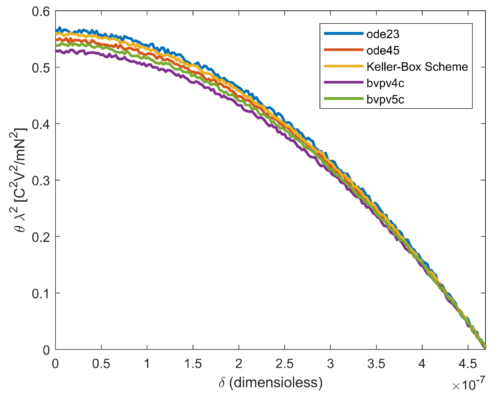
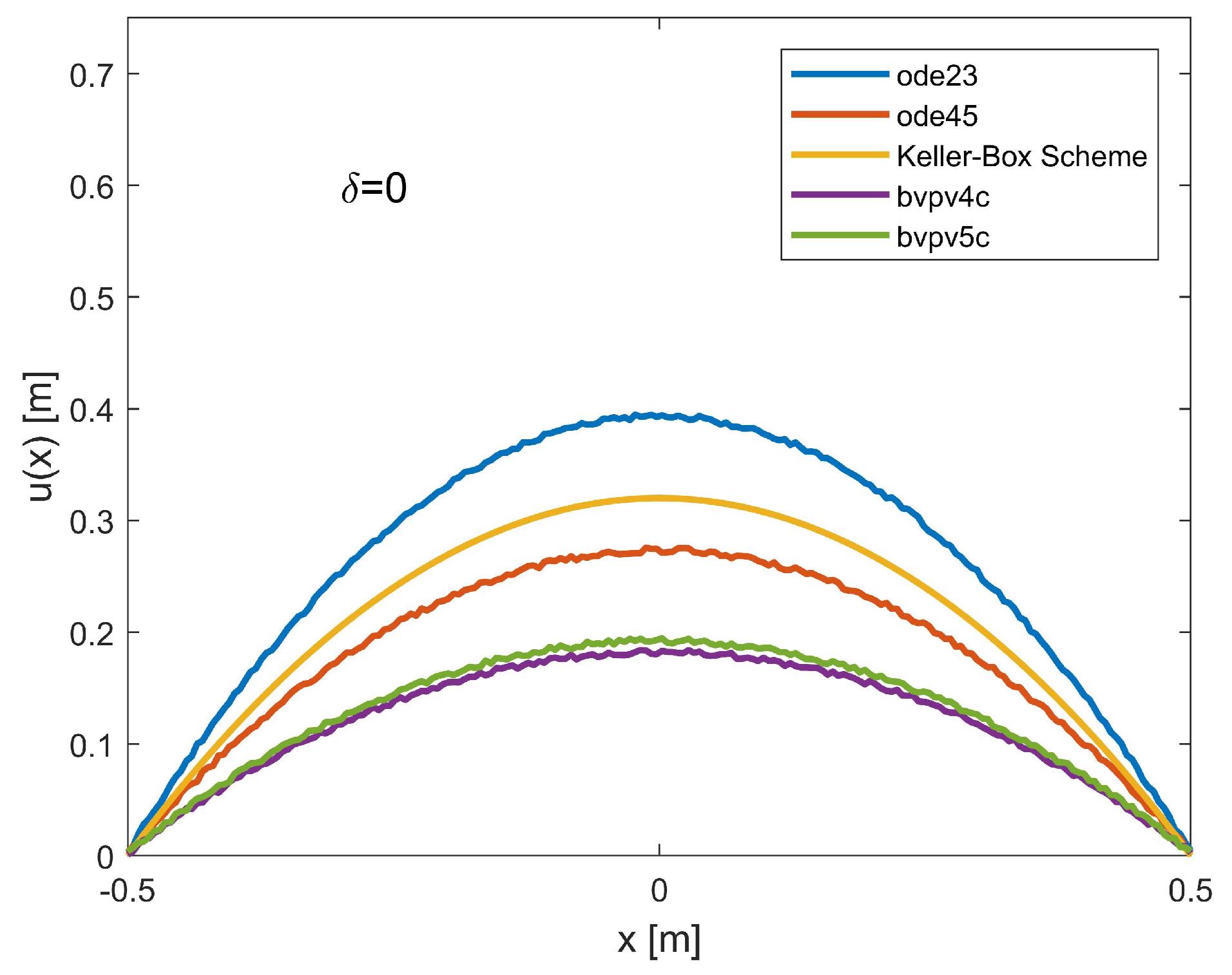
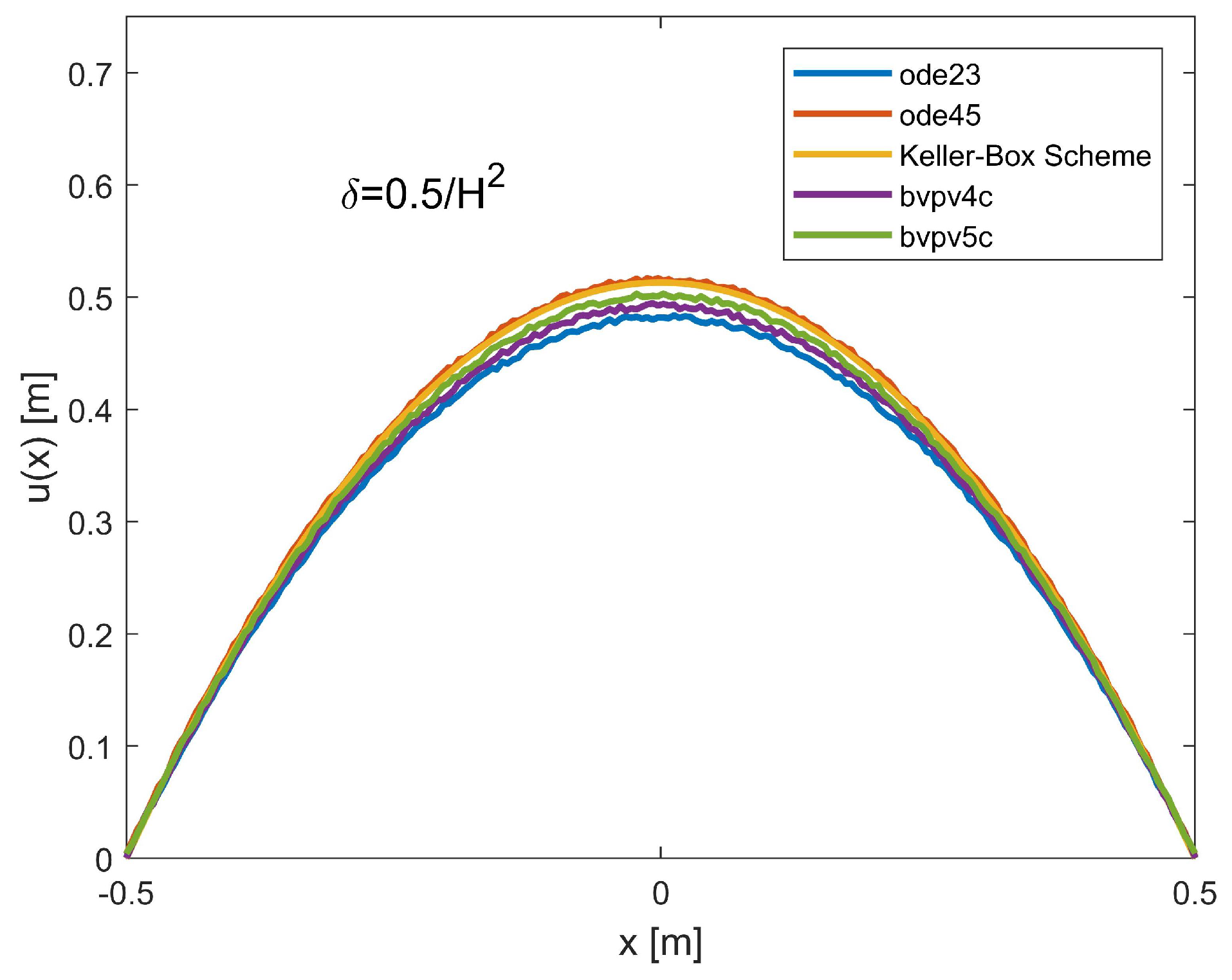
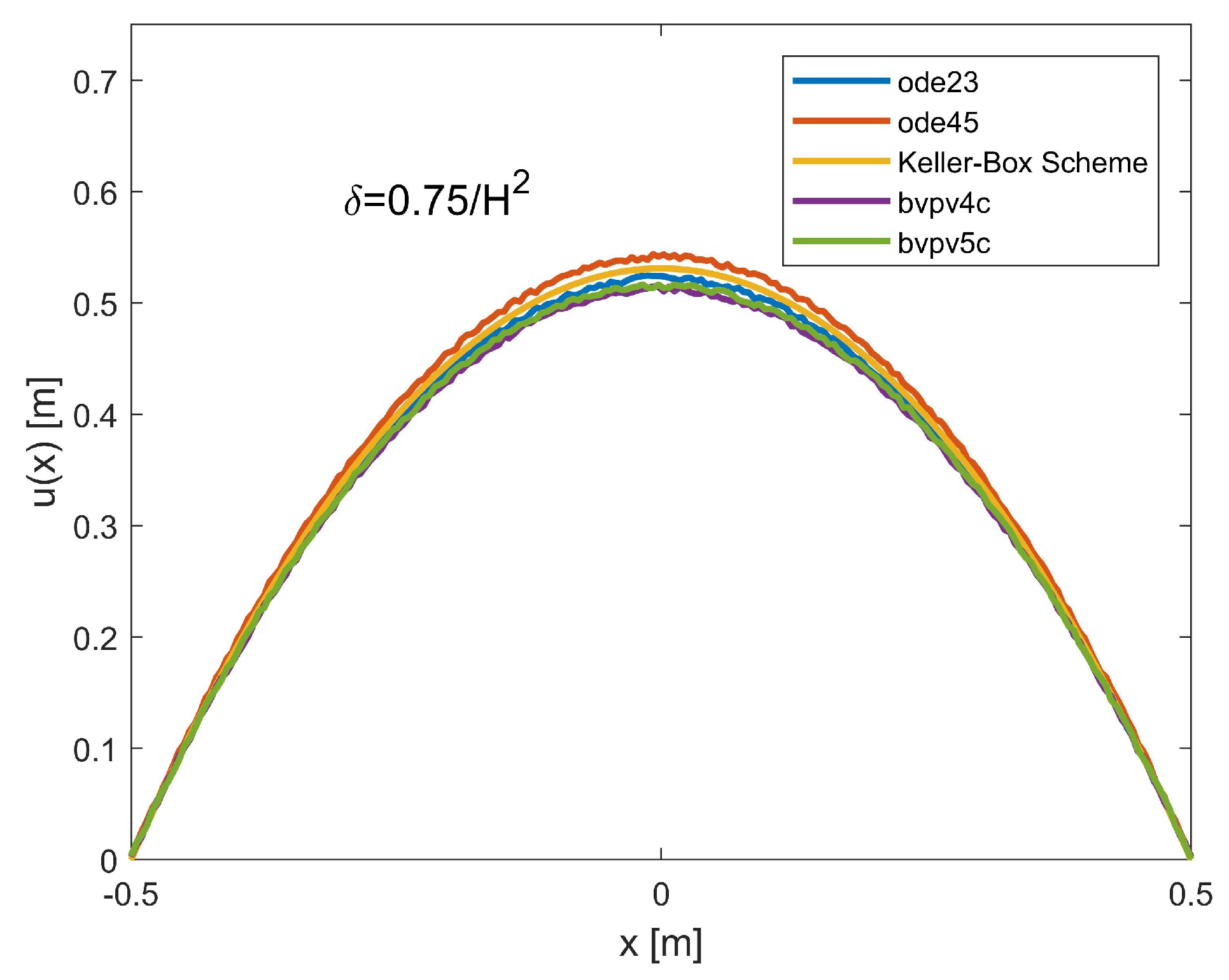
Furthermore, in Figure 4, for each procedure used, the trends of have been plotted as a function of the admissible . From this figure, we can see how these trends agree with the trends anticipated in Table 1. However, this further highlights that as we move towards small values (i.e., towards reduced fringing field effects), a slight discrepancy of takes place. We observe that, when (in the absence of a fringing field) the convergence of all numerical techniques, without ghost solutions, is ensured if . When increases, strongly decreases, reaching . Therefore, according to Remark 21, the membrane deforms further. For example, Figure 5, Figure 6, Figure 7, Figure 8 and Figure 9 depict the recovery of the membrane profile as increases (in its range of possible values) for a value of , which still ensures the convergence of all numerical procedures (in the absence of ghost solutions).
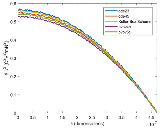
Figure 4.
Numerical reconstruction of the trend of as the effect due to the fringing field increases (in convergence conditions and without ghost solutions).

Figure 5.
Profile recovery for (in the absence of a fringing field, in convergence conditions, and without ghost solutions).
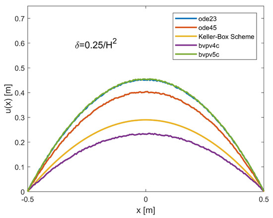
Figure 6.
Profile recovery for (in convergence conditions and without ghost solutions).

Figure 7.
Profile recovery for (in convergence conditions and without ghost solutions).
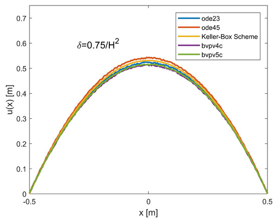
Figure 8.
Profile recovery for (in convergence conditions and without ghost solutions).
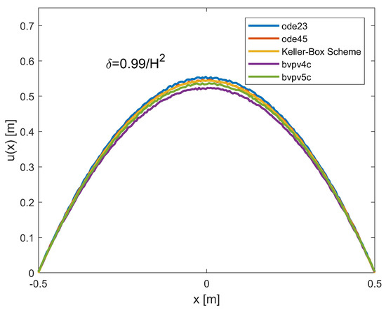
Figure 9.
Profile recovery for (in convergence conditions and without ghost solutions).
Remark 22.
Even if δ increases in its range of possible values and decreases (always ensuring the convergence of all numerical procedures in the absence of ghost solutions), there is a prevalence of the effect due to δ, as enshrined in the model under study. This is because the profile increases its concavity when δ increases because favors the deformation of the membrane towards the upper plate.
Remark 23.
We highlight that the Keller box scheme provides the best performance in terms of recovering the membrane profile. This is evident from the figures, where the profile of the membrane recovered using the Keller box scheme is more regular than those obtained with the other procedures. However, the Keller box scheme has a higher computational complexity than the other numerical procedures [30], making this procedure unattractive for any real-time industrial applications where very short membrane recovery times are required. Fortunately, such industrial applications are not yet widespread, so the Keller box scheme currently represents the “gold standard” for obtaining approximate solutions of these particular types of analytical models. However, a clarification is needed regarding the choice of the number of nodes, N. Regarding the Keller box and Lobatto procedures, was chosen to have the same number of nodes automatically selected by . When , on the one hand, the Keller box method does not converge and, on the other hand, Lobatto’s performance does not reach the desired accuracy, showing highly irregular membrane profiles.
Remark 24.
The usefulness of using multiple numerical procedures with different convergence characteristics to recover the membrane profile arises from the need to highlight the effectiveness and efficiency of each single numerical approach consolidated in the scientific literature for this type of analytical model. Obviously, the recovered profiles are qualitatively comparable, even though there are small differences attributable to the different orders of accuracy of the numerical procedures used.
11. On the Limitation for and a Reliable Value of to Overcome the Membrane Inertia
We may recall that (122) and (123) are operationally uninteresting. Thus, according to Remark 19, we present the following result.
Proposition 6.
Indicating by
the value of in convergence conditions, below which ghost solutions occur
Moreover, removing the dependency on x, (130) becomes
We report here the proof of this proposition because, as above, it proposes interesting computations concerning the fringing field.
Proof.
From the equation of the model under study, we can easily state
from which, considering (12), we achieve
Condition (130) is physically interesting because it provides a limitation for T depending on x. However, operationally, it is more convenient to use (131), where the dependence on is intrinsic in . Furthermore, the dependence of T on is guaranteed by the presence of . Finally, it is clear that, with a fixed L, membranes with higher T values can be installed in devices with closely spaced plates (i.e., devices with small d values). This is because a greater T will hardly allow the membrane to touch the upper plate. Conversely, at fixed d, membranes with a reduced value of T can be installed in devices of which the plates have a small L.
Moreover, with being constant and setting the geometry of the device a priori (i.e., setting both L and d), from (131) we can state:
where
In other words, once is attributable (according to the desired effects due to the fringing field) K is fixed, so that the curve
is selected (see Figure 10). Then, once V is chosen (i.e., once the intended use of the device is chosen), the line parallel to the ordinate axis and passing through the point is fixed; this line intercepts the curve at a point for which all the points below it and belonging to the aforementioned line represent T values that are admissible for that particular intended use of the device.
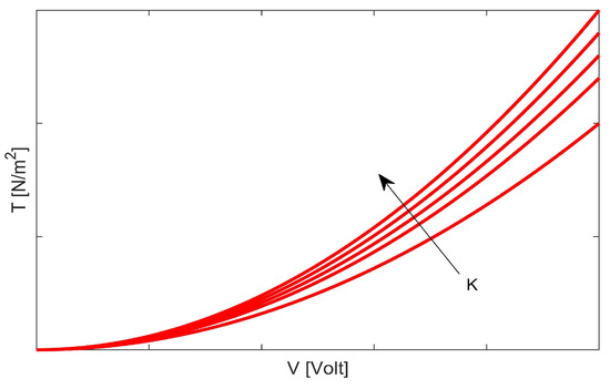
Figure 10.
Geometric link between T and V.
Conversely, under analog reasoning, the same graph depicted in Figure 10 can be used to choose the intended use of a particular device.
12. On the Influence of Electromechanical Properties on the Proposed Procedure
The proposed procedure has a physical-engineering comparison that needs to be further clarified in the following items.
- Both recovering the membrane profile numerically and obtaining the limitations for T and for V strongly depend on the electromechanical properties of the material constituting the membrane. In fact, the prevailing presence of throughout the procedure highlights this dependence. In particular, we have seen how the presence in the denominator of in the starting analytical model influences and therefore the concavity of the membrane profile, in the sense that the greater (i.e., the greater T) the lower the concavity of the membrane. From the physical point of view, this translates into the fact that the higher the T, the greater the mechanical resistance that the membrane offers to deformation.
- On the other hand, as confirmed by (29), the higher the T (i.e., with values less than ) the lower the H, so it is confirmed that more resistant membranes will cause deformations that are more contained to the edges.
- Moreover, as it should be, also strongly influences the conditions of existence and uniqueness of the solution for the model under study (see (35)).
- It is worth underlining the fact that the proposed procedure is based on numerical techniques of which the convergences depend exclusively on . In other words, it is the electromechanical properties of the membrane material that “manage” the convergences of the numerical techniques used and ensure that the membrane profile obtained does not represent a ghost solution, regardless of the value of the parameter that weights the effect due to the fringing field, though obviously within the range of its possible values, (see (127)).
- Furthermore, (139) highlights how the electromechanical properties of the material constituting the membrane once again influence the choice of T. In other words, having chosen the intended use of the device (that is, choosing an external V to apply), directly affects the value of T. Vice versa, having selected a specific value of T (that is, having chosen the material of which the membrane must be constituted), from (139), it is possible to establish the intended use of the device.
- It is worth noting that from derives an important link between (which is the parameter that weighs the effects due to the fringing field) and the ratio . In fact, based on (126), and taking into account (12), it easily follows that:in whichandwith . In other words, after one has fixed the length L of the device and the material constituting the membrane (that is, once T is fixed), explicitly depends on , as evidenced by (144). Thus, as confirmed by the experimental facts, the higher the ratio (i.e., L/d 1), the less the effects due to the fringing field will be. However, in the current state of modeling, as it is one-dimensional, we can say nothing about the dependence of on the ratio , where w is the width of the device. We arrive at the same conclusions starting from (135).
13. Destinations of Use of the Device Studied
The MEMS membrane device here presented and studied does not require sophisticated precautions for its implementation in software and its hardware prototyping. Furthermore, it is our opinion that its large-scale industrial implementation would require very low costs. Once the device has been made, it can be used in biomedical applications, where the operating voltage V is limited (see (6)), for example, in micro-pumps for drug delivery systems and precision surgical micro-systems. Obviously, it is necessary to have an effective and efficient control circuit (for example, a capacitive circuit) that is capable of interfacing with functional systems in which the MEMS can be interfaced. Finally, we observe that MEMS devices are equipped not only with electronic parts, but also with mechanical parts (which require specific tests) integrated in a single chip (combining microelectronics with the mechanics of microsensors), which is attractive, for example, for robotics in metropolitan areas of smart cities.
14. Conclusions and Perspectives
The study of a semi-linear elliptic II-order 1D differential model of a membrane MEMS device, previously described in the literature, in which was shown to be locally proportional to the geometric curvature of the membrane, has been thoroughly explored here. In the model, there is a term proportional to , which takes into account the effects due to the fringing field. Starting from the advantages and disadvantages that the model has, a new algebraic condition has been presented here, ensuring the existence and uniqueness of the solution depending on the electromechanical characteristics of the material constituting the membrane and on the parameter that weights such effects. Moreover, the fringing field’s influence on the device’s electrostatic force has been studied. However, we observed that is not explicitly controllable in terms of voltage; therefore, it would be useful in the future to study the possibility of controlling this parameter by means of V in order to avoid any unwanted electric discharges in the dielectric. Furthermore, it is desirable in the near future to be able to highlight the important dependence of on the length/width ratio of the device in order to offer a broad comparison with the advanced experimentation of devices in the industrial field. Since the model does not allow the membrane profiles to be obtained explicitly, numerical techniques considered the “gold standard” for the numerical resolution of analytical models such as the one under study were used and compared, obtaining, on the one hand, a useful range of admissible values for the parameter governing the convergence of numerical procedures in the absence of ghost solutions and, on the other, reliable membrane profiles. Finally, a new criterion for the choice of the membrane material, starting from the electrostatic operating parameters of the device (and vice versa), was presented and discussed. Finally, we note how the presence of ordinary derivatives in the model does not require the use of FEM techniques which, notoriously, have excellent performance with partial or ordinary derivative models of which the numerical models are built on two-dimensional meshes (for example, dynamic models in which the time variable is present). Therefore, in the future, we intend to reformulate the model so that it can be studied numerically by means of FEM techniques which are highly useful for hardware prototyping. Furthermore, it is desirable to obtain an algebraic condition of existence and uniqueness that is dependent both on the electrical conductivity of the material constituting the membrane and on the temperature, to highlight any bifurcation phenomena and, if possible, to establish the conditions of existence and uniqueness for dynamic investigations. We note the fact that, at present, the authors are studying the 3D generalization of the model presented here. As soon as the theoretical results are in line with the experimentation in the laboratory, it will be our responsibility to make known the salient features of the research. Finally, it is worth noting that the technique used here, which uses an algebraic condition of existence and uniqueness to obtain the limitation for T and the minimum value of V, is difficult to use in any applications since, strictly speaking, it would be necessary to select the minimum value among all values that would ensure the convergence of each numerical procedure. Furthermore, it would also be necessary to evaluate (see related proof), which, at present, has a mainly theoretical value. Therefore, in the near future it will be necessary to work to make this important tool more usable.
Author Contributions
Conceptualization, M.V. and P.D.B.; methodology, M.V. and P.D.B.; software, M.V. and P.D.B.; validation, M.V. and P.D.B.; formal analysis, M.V. and P.D.B.; writing—original draft preparation, M.V.; writing—review and editing, P.D.B. All authors have read and agreed to the published version of the manuscript.
Funding
This research received no external funding.
Institutional Review Board Statement
Not applicable.
Informed Consent Statement
Informed consent was obtained from all subjects involved in the study.
Conflicts of Interest
The authors declare no conflict of interest.
Abbreviations
The following abbreviations are used in this manuscript:
| MEMS | microelectromechanical systems |
| x | spatial abscissa ((m)) |
| profile of the membrane ((m)) | |
| bounded domain | |
| electrostatic field ((V/m)) | |
| critical security distance ([m]) | |
| real positive parameter that weights the effect due to the fringing field (dimensionless) | |
| d | distance between the parallel plates ((m)) |
| L | length of the MEMS ((m)) |
| V | external electric voltage applied ((V)) |
| permittivity of the free space ((C2/Nm3)) | |
| electrostatic pressure ((N/m2)) | |
| electrostatic force ((N)) | |
| T | mechanical tension of the membrane at rest ((N/m2)) |
| density ((kg/m3)) | |
| D | stiffness coefficient ((N/m)) |
| p | mechanical pressure ((N/m2)) |
| electrostatic capacitance ((F)) | |
| k, | coefficients of proportionality (dimensionless) |
| self-stretching coefficient (dimensionless) | |
| coefficient of stretching energy (dimensionless) | |
| stretching parameter (dimensionless) | |
| bounded functions which carries the dielectric properties of the material constituting the membrane (dimensionless) | |
| parameter depending on the electrostatic capacitance (dimensionless) | |
| capacitor belonging to the control circuit ((F)) | |
| drop-voltage ([C2V2/mN2]) | |
| real parameter that weights the effects due to the fringing field (dimensionless) | |
| Pelesko–Driskoll fringing function | |
| coefficient of proportionality (dimensionless) | |
| geometric curvature of the membrane ((m−1)) | |
| function of proportionality (dimensionless) | |
| electromechanical properties of the material constituting the membrane (C2V2/mN2) | |
| H | (dimensionless) |
| real positive parameter (dimensionless) | |
| fringing field ([V/m]) |
References
- Pelesko, J.A.; Bernstein, D.H. Modeling MEMS and NEMS; Chapman & Hall/CRC: Boca Raton, FL, USA; London, UK; New York, NY, USA; Washington, DC, USA, 1998. [Google Scholar]
- Gad-el-Hak, M. Design and Fabrication; Chapman & Hall/CRC: Boca Raton, FL, USA; London, UK; New York, NY, USA; Washington, DC, USA, 2006. [Google Scholar]
- Ghodssi, R.; Lin, P. MEMS Materials and Processes Handbook; Springer: Boston, MA, USA, 2011. [Google Scholar]
- Younis, M.I.; Nayfeh, A.H. A Study of the Nonlinear Response of a Resonant Microbeam to an Electric Actuation. Nonlinear Dyn. 2003, 31, 91–117. [Google Scholar] [CrossRef]
- Morabito, F.C. Independent Component Anaysis and Feature Extraction Techniques for NDT Data. Mater. Eval. 2000, 58, 85–92. [Google Scholar]
- Greco, A.; Costantino, D.; Morabito, F.C.; Versaci, M. A Morlet Wavelet Classification Technique for ICA Filtered sEMG Experimental Data. Modeling and Simulation of MEMS Components: Challenges and Possible Solutions, Micromachining Techinques for Fabrication of Micro and Nano Structures, Portland, OR, USA, 20–24 July 2003; pp. 166–171. [Google Scholar]
- Gad-el-Hak, M. Modeling and Simulation of MEMS Components: Challenges and Possible Solutions, Micromachining Techinques for Fabrication of Micro and Nano Structures; Springer Nature: Singapore, 2012. [Google Scholar]
- De Holiveira Hansen Noble, R.; Mária, M.; Romans, S.; Jost, A.; Steffen, C.; Tim, R.; Bernhard, W.; Wolfgang, B.; Stefan, M. Magnetic Fils for Electromagnetic Actuation in MEMS Switches. Microsyst. Technol. 2018, 24, 529–551. [Google Scholar]
- Zhu, J. Development Trends and Perspectives of Future Sensors and MEMS/NEMS. Micromachines 2020, 11, 7. [Google Scholar] [CrossRef] [PubMed] [Green Version]
- Ren, Z.; Chang, Y.; Ma, Y.; Shih, K.; Dong, B.; Lee, C. Leveraging of MEMS Technologies for Optical Metamaterials Applications. Adv. Opt. Mater. 2019, 8, 1900653. [Google Scholar] [CrossRef]
- Lee, S.; Chen, C.; Deshp, V.V.; Lee, G.H.; Lee, I.; Lekas, M. Electrically Integrated SU-8 Clamped Graphene Drum Resonators for Strain Engineering. Appl. Phys. Lett. 2013, 102, 153101. [Google Scholar] [CrossRef] [Green Version]
- Fan, X.; Smith, A.D.; Forsberg, F.; Wagner, S.; Schröder, S.; Akbari, S.S.A.; Fischer, A.C.; Villanueva, L.G.; Östling, M.; Lemme, M.C.; et al. Manufaccture and Characterization of Graphene Membranes with Suspended Silicon Proof Masses for MEMS and NEMS Applications. Microsyst. Nanoeng. 2020, 102, 17. [Google Scholar] [CrossRef] [Green Version]
- Zhou, X.; Venkatachalam, S.; Zhou, R.; Xu, H.; Pokharel, A.; Fefferman, A. High-Q Silicon Nitride Drum Resonators Strongly Coupled. Nano Lett. 2021, 21, 5738–5744. [Google Scholar] [CrossRef]
- Phan, A.; Truong, P.; Schade, C.; Joslin, K.; Talke, F. Analytical Modeling of an Implantable Opto-Mechanical Pressure Sensor to Study Long Term Drift. In Proceedings of the ASME 2020 29th Conference on Information Storage and Processing Systems, Virtual, 24–25 June 2020; p. V001T06A003. [Google Scholar]
- Yen, Y.K.; Chiu, C.Y. A CNOS-MEMS-Based Membrane-Bridge Nanomechanical Sensors for Small Molecule Detection. Sci. Rep. 2020, 10, 5237. [Google Scholar] [CrossRef]
- Ma, T.; Cao, H.; Shen, C. A Temperature Error Parallel Processing Model for MEMS Gyroscope based on a Novel Fusion Algorithm. Electronics 2020, 9, 499. [Google Scholar] [CrossRef] [Green Version]
- Wang, D.; Watkins, C.; Xie, H. MEMS Mirrors for LiDAR: A Review. Micromachines 2020, 11, 456. [Google Scholar] [CrossRef] [PubMed]
- Javaher, H.; Ghanati, P.; Azizi, S. A Case Study on the Numerical Solution and Reduced Order Model of MEMS. Sens. Imaging 2018, 19, 153–169. [Google Scholar] [CrossRef]
- Versaci, M.; Jannelli, A.; Morabito, F.C.; Angiulli, G. MEMS Device considering the Effect of the Fringing Field. Sensors 2021, 21, 5237. [Google Scholar] [CrossRef]
- Hashimoto, K.; Shiotani, T.; Mitsuya, H.; Chang, K.C. MEMS Vibrational Power Generator for Bridge Slab and Pier Health Monitoring. Appl. Sci. 2020, 10, 8258. [Google Scholar] [CrossRef]
- Versaci, M.; Di Barba, P.; Morabito, F.C. Curvature-Dependent Electrostatic Field as a Principle for Modelling Membrane-Based MEMS Devices. A Review. Membranes 2020, 10, 361. [Google Scholar] [CrossRef]
- Chen, S.J.; Chen, B. Research on a CMOS-MEMS Infrared Sensor with Reduced Graphene Oxide. Sensors 2020, 20, 4007. [Google Scholar] [CrossRef]
- Di Barba, P.; Fattorusso, L.; Versaci, M. Curvature-Dependent Electrostatic Field as a Principle for Modelling Membrane MEMS Device with Fringing Field. Comput. Appl. Math. 2021, 40, 87. [Google Scholar] [CrossRef]
- Versaci, M.; Di Barba, P. Deformable MEMS with Fringing Field: A New Uniqueness Condition for Identifying the Electrode Profile. In Proceedings of the 20th International Symposium on Electromagnetic Fields in Mechatronics, Electrical and Electronic Engineering, Lodz/Cracow, Poland, 20–23 September 2021. [Google Scholar]
- Versaci, M.; Jannelli, A.; Angiulli, G. Electrostatic Micro-Electro-Mechanical-Systems (MEMS) Devices: A Comparison Among Numerical Techniques for Recovering the Membrane Profile. IEEE Access 2020, 8, 125874–125886. [Google Scholar] [CrossRef]
- Pelesko, J.A.; Driscoll, T.A. The Effect of the Small-Aspect-Ratio Approximation on Canonical Electrostatic MEMS Models. J. Eng. Math. 2005, 53, 239–252. [Google Scholar] [CrossRef] [Green Version]
- Cassani, D.; Ghoussoub, N. On a Fourth Order Elliptic Problem with a Singular Nonlinearity. Adv. Nonlinear Stud. 2011, 9, 189–209. [Google Scholar] [CrossRef]
- Jonassen, N. Electrostatics; Springer: Singapore, 2014. [Google Scholar]
- Bayley, P.B.; Shampine, L.F.; Waltman, P.E. Nonlinear Two Points Boundary Value Problems; Academic Press: London, UK, 1969. [Google Scholar]
- Kress, R. Numerical Analysis; Springer: New York, NY, USA, 1998. [Google Scholar]
- Versaci, M.; Di Barba, P.; Morabito, F.C. MEMS With fringing Field: Curvature-Dependent Electrostatic Field and Numerical Techniques for Recovering the Membrane Profile. Comput. Appl. Math. 2021, 40, 128. [Google Scholar] [CrossRef]


Publisher’s Note: MDPI stays neutral with regard to jurisdictional claims in published maps and institutional affiliations. |
© 2022 by the authors. Licensee MDPI, Basel, Switzerland. This article is an open access article distributed under the terms and conditions of the Creative Commons Attribution (CC BY) license (https://creativecommons.org/licenses/by/4.0/).