Radiation Pattern Synthesis of the Coupled almost Periodic Antenna Arrays Using an Artificial Neural Network Model

Abstract

This paper proposes radiation pattern synthesis of almost periodic antenna arrays including mutual coupling effects (extracted by Floquet analysis according to our previous work), which in principal has high directivity and a large bandwidth. For modeling the given structures, the moment method combined with the generalized equivalent circuit (MoM-GEC) is proposed. The artificial neural network (ANN), as a powerful computational model, has been successfully applied to antenna array pattern synthesis. Our results showed that multilayer feedforward neural networks are rugged and can successfully and efficiently resolve various distinctive, complex almost periodic antenna patterns (with different source amplitudes) (in particular, both periodic and randomly aperiodic structures are taken into account). An ANN is capable of quickly producing the synthesis results using generalization with the early stopping (ES) method. Significant advantages in speed and memory consumption are achieved by using this method to improve the generalization (called early stopping). To justify this work, several examples are shown and discussed.

1. Introduction

Today, the synthesis of the radiation patterns of almost periodic planar structures is the subject of research, mostly in space and defense applications, communication systems and electronic devices such as phased array radar systems, frequency selective surface (FSS) applications  [1], millimeter waves, and optical wave regions (other examples: reflection gratings, phased arrays, electromagnetic bandgap structures, leaky wave antennas, etc...) [2,3,4,5].

In general, smart antenna arrays involve intelligent systems, including genetic algorithms and neural networks, to synthesize the radiation pattern [6,7,8,9,10]. The genetic algorithm (GA) is used basically for sidelobe reduction in antenna pattern synthesis [11,12,13]. As well, artificial neural networks (ANNs) have been employed for various purposes, e.g., as pattern recognition systems, and have been put to use for input–output mapping, system identification, adaptive prediction, etc. Consequently, the present work is centered on a neural network technique for the synthesis of almost periodic network models, and we point out their most prominent features and distinctive characteristics [14,15,16].

Several other methods of synthesis of coupled periodic and aperiodic arrays have shown their reliability in electromagnetic calculations [17,18], one of which is MoM GeC, which we use as a comparison method herein.

Other methods based on machine learning have been shown to simplify the electromagnetic calculations and to approximate with great accuracy the electronic performances of coupled, decoupled, periodic, and aperiodic arrays [19,20,21,22,23,24,25,26,27,28,29,30,31,32,33].

Our objective was to develop a feedforward neural network with supervised training to approximate the function of a radiation pattern which is provided by the method of moments and simplified by an equivalent circuit scheme.

For clarity, this paper presents some basic details on the optimum size of a feedforward neural network to prevent overfitting problems. Next, we describe how we divided the radiation model datasets for training, testing, and validation. Then, we describe how the feedforward neural network was generated and trained [34]. We report how the output values were generated and denormalized; and finally, the neural network’s performance is examined by checking the output values against the numerical target values [15,16].

The equivalent circuit scheme reduces the complexness of the problem by setting and adapting the neural network patterns, such as training, architecture, and parameters, which will enhance and give more accurate input–output relations [13]. Our main idea here is to address the synthesis of antenna arrays for coupled almost periodic array geometries, especially future complex extended aperiodic configurations [35,36].

This paper is organized as follows: In Section 2, the fundamental theoretical background of the numerical analysis, including the computation of the radiation field, is recalled, particularly for almost periodic arrays. In relation to the synthesis of a radiation pattern, the basic concepts of artificial neural networks (ANNs) and their applications are recalled in Section 2. Some fundamental networks are examined in detail for their capability to deal with the problem of simple pattern synthesis. Then, we describe the development and construction of new architectures for the synthesis of complex almost periodic antenna arrays (e.g., randomly aperiodic phased arrays). The next section presents the numerical results and discussion. In the last section, some conclusions are presented.

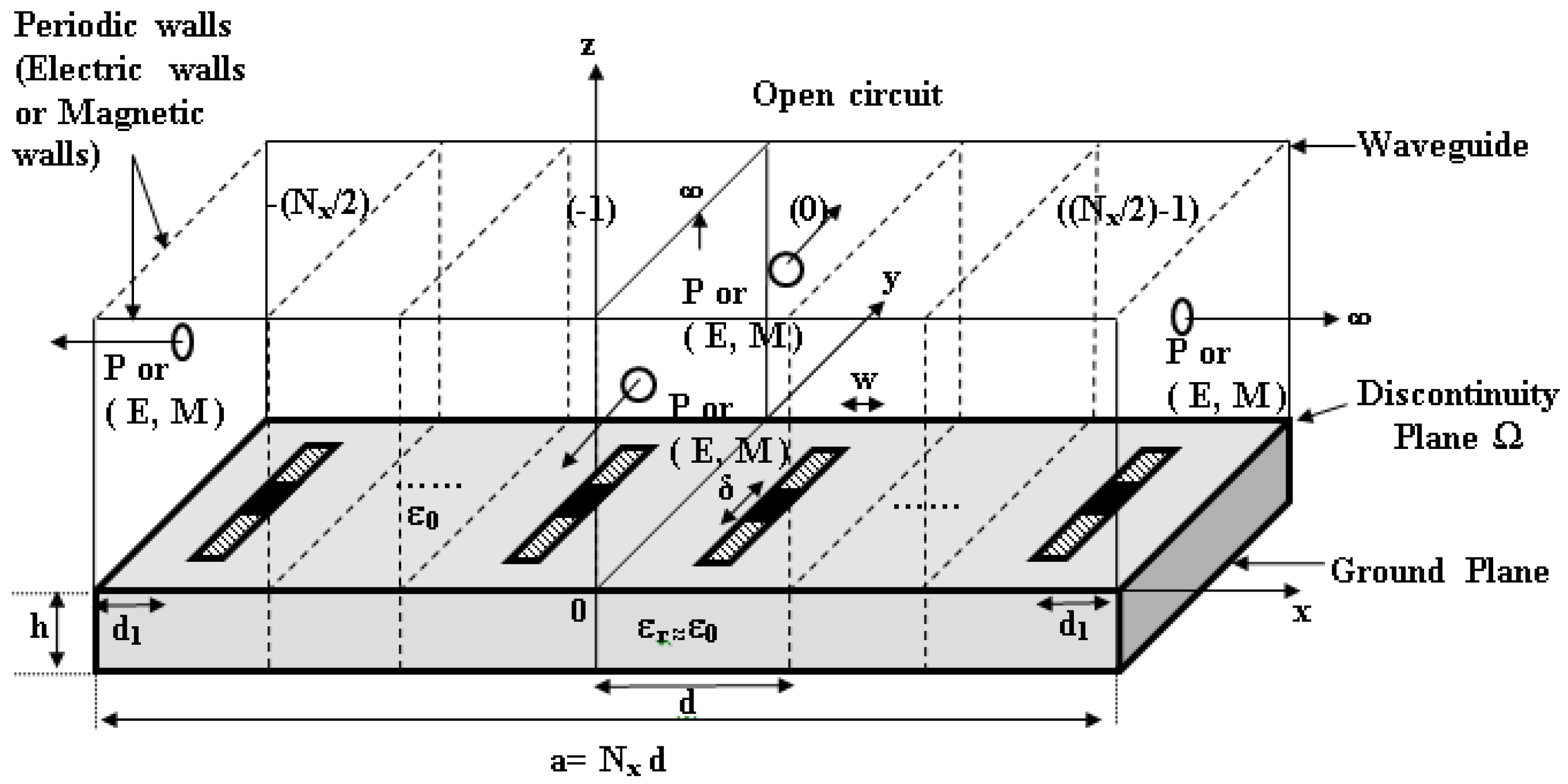
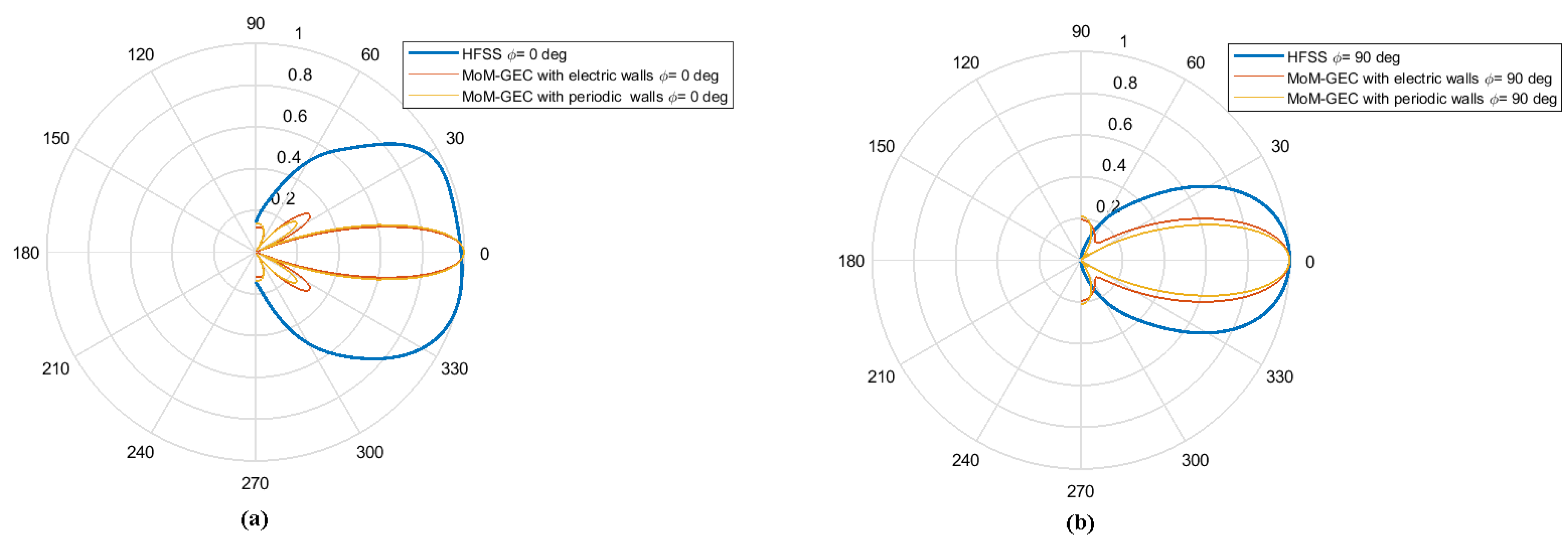
2. Problem Formulation: (Radiation Patterns of the Almost Periodic Structures)

This section shows the main expression of the radiation pattern related to the proposed almost periodic planar structures (see Figure 1 for the periodic antenna array example) [37,38,39], which was discussed in our previous work [2,3,5]. To extract such a radiation pattern, it is claimed that an integral method based on the method of moments combined with the generalized equivalent circuit (MoM-GEC) [37,38,40] should be implemented.

Therefore, the relation of the total near-field distribution set on the surface of the discontinuity (rectangular opening aperture) (metal form + dielectric substrate) of the global almost periodic structures can be defined according to the Galerkin procedure as follows [4,37,38,39]:

• On the metallic part, the electric field can be given by:

$$|E(x,y)\rangle =\sum _p\sum _q{\left[Z\right]}_{pq}{X}_{pq}|g_{pq}\rangle$$

(1)

• On the discontinuity plane (or on the radiating aperture), the electric field is expressed in function of the guide’s modes as:

$$|E(x,y)\rangle =\sum _{m,n}\sum _p\sum _q{\left[Z\right]}_{pq}{X}_{pq}\langle f_{mn}|g_{pq}\rangle |f_{mn}\rangle$$

(2)

with:

$$[{\widehat{Z}}_{pq,st}^{upper,down}]=[\sum _{m,n}\langle g_{pq}|f_{mn}\rangle z_{mn}^{upper,down}\langle f_{mn}|g_{st}\rangle ]$$

(3)

and the inner product is yielded by:

$$\langle u|v\rangle =\int {\int }_{D}u{v}^{*}ds$$

(4)

(* refers to the complex conjugate).

$|f_{mn}\rangle$ denotes the modes $|T{E}_{mn}\rangle$, $|T{M}_{mn}\rangle$.

$|g_{pq}\rangle$ indicates the test functions used and $X_{pq}$ the inconnue weights of this function to be evaluated and ${\tilde{z}}_{mn}$ are the total modal impedance related to the guide modes.

A specific selection of test functions must be used to express the unknown current density established on the metal parts of the selected structures.

Based on the Fourier transform, the far field of the given total structure can be written as:

$$\begin{array}{c}\hfill {\tilde{E}}_{x,y,{\theta }_0,{\varphi }_0}(\theta ,\varphi )={\int }_{-c}^c\{{\int }_0^L{E}_{aperture}(x,y)\\ \hfill e^{\left(j{k}_0(sin\left(\theta \right)cos\left(\varphi \right)-sin\left({\theta }_0\right)cos\left({\varphi }_0\right))x\right)}dx\}\\ \hfill e^{\left(j{k}_0(sin\left(\theta \right)sin\left(\varphi \right)-sin\left({\theta }_0\right)sin\left({\varphi }_0\right))y\right)}dy.\end{array}$$

(5)

$E_{aperture}(x,y)$ is obtained by a spatial calculation with the MoM method. The pair (${\theta }_0,{\varphi }_0$) is seen as the orientation direction of the main beam (steering direction) and the pair ($\theta ,\varphi$) indicates the shape of the radiation pattern.

Note that a midpoint sum approximating double integrals is used to compute the far-field (refering to Appendix A), followed by a Matlab source code that explains how to implement it with the MoM GEC, as given in Appendix B.

To restrain the electromagnetic calculation to one unit cell, the dependence on Floquet modes ($\alpha$ or $(\alpha ,\beta )$) is taken into account [2,3,4,36]. Then, the field components can be expressed in generalized Fourier series expansions, and the analysis region can be reduced to only one periodicity cell bounded by the known periodic walls, as presented in Figure 2 [41,42]. In this case, the interaction between cells can be taken into consideration using a novel expression of the mutual coupling shown in the previous work [2,3]. All details about the electromagnetic modal calculation based on the Floquet analysis are proven in [2,3,4]. To remind the reader of the radiating pattern expression ${\tilde{E}}_{x,y}(\theta ,\varphi )$ developed through the modal decomposition in the spectral domain, we detail the steps given below [4]:

The total electric field radiated by the structure is:

$$E{(x,y)}_{aperture}=\frac{1}{\sqrt{N_x{N}_y}}\sum _{p=-\frac{N_x}{2},q=-\frac{N_y}{2}}^{\frac{N_x}{2}-1,\frac{N_y}{2}-1}{\tilde{E}}_{{\alpha }_p,{\beta }_q,aperture}(x,y)e^{j{\alpha }_p\left(i{d}_x\right)}{e}^{j{\beta }_q\left(s{d}_y\right)}$$

(6)

Then, the normalized radiating pattern is given by:

$$\begin{array}{c}\hfill {\tilde{E}}_{x,y,{\theta }_0,{\varphi }_0}(\theta ,\varphi )==\frac{1}{\sqrt{N_x{N}_y}}\sum _{i=-\frac{N_x}{2},s=-\frac{N_y}{2}}^{\frac{N_x}{2}-1,\frac{N_y}{2}-1}\\ \hfill E_{aperture}(x,y)e^{\left(j{k}_0(sin\left(\theta \right)cos\left(\varphi \right)-sin\left({\theta }_0\right)cos\left({\varphi }_0\right))i{d}_x\right)}\\ \hfill e^{\left(j{k}_0(sin\left(\theta \right)sin\left(\varphi \right)-sin\left({\theta }_0\right)sin\left({\varphi }_0\right))s{d}_y\right)}\end{array}$$

(7)

Moreover, the far radiating field in the Floquet domain when the $z>0$ region, is written as follows:

$$\begin{array}{c}\hfill {\tilde{E}}_{x,y}^{\alpha ,\beta }(\theta ,\varphi )={\int }_{-c}^c\{{\int }_0^L{E}_{aperture}^{\alpha ,\beta }(x,y)\\ \hfill e^{\left(j{k}_0(sin\left(\theta \right)cos\left(\varphi \right)-sin\left({\theta }_0\right)cos\left({\varphi }_0\right))x\right)}dx\}\\ \hfill e^{\left(j{k}_0(sin\left(\theta \right)sin\left(\varphi \right)-sin\left({\theta }_0\right)sin\left({\varphi }_0\right))y\right)}dy\end{array}$$

(8)

After that, the expression of the directivity (in Floquet space) is obtained as [43]:

$$D_{\alpha ,\beta }({\varphi }_0,{\theta }_0)=\frac{|{\tilde{E}}_{\alpha ,\beta }({\varphi }_0,{\theta }_0){|}^2}{\frac{1}{4\pi }{\int }_0^{2\pi }{\int }_0^{\pi }{\left|{\tilde{E}}_{\alpha ,\beta }(\theta ,\varphi )\right|}^{2}sin\left(\theta \right)d\varphi d\theta }$$

(9)

Therefore, to study the spatial electromagnetic behavior of periodic antenna arrays (as explained in the previous section in Equation (5)), another way to proceed is based on the superposition of Floquet states (superposition theorem) in a finite or infinite periodic array:

• For small and large finite arrays:

We must indicate that the Floquet states are considered discrete (with their physical fields):

The spatial electric and current fields are deduced as:

$$\begin{array}{c}\hfill E(i{d}_x,k{d}_y)=\frac{1}{\sqrt{N_x{N}_y}}\sum _{p=-\frac{N_x}{2}}^{\frac{N_x}{2}-1}\sum _{q=-\frac{N_y}{2}}^{\frac{N_y}{2}-1}{\tilde{E}}_{aperture}^{{\alpha }_p,{\beta }_q}(x,y)\\ \hfill e^{j{\alpha }_p\left(i{d}_x\right)}{e}^{j{\beta }_q\left(k{d}_y\right)}\end{array}$$

(10)

$$\begin{array}{c}\hfill J(i{d}_x,k{d}_y)=\frac{1}{\sqrt{N_x{N}_y}}\sum _{p=-\frac{N_x}{2}}^{\frac{N_x}{2}-1}\sum _{q=-\frac{N_y}{2}}^{\frac{N_y}{2}-1}{\tilde{J}}_{aperture}^{{\alpha }_p,{\beta }_q}(x,y)\\ \hfill e^{j{\alpha }_p\left(i{d}_x\right)}{e}^{j{\beta }_q\left(k{d}_y\right)}\end{array}$$

(11)

Then, the total radiating electric field is:

$$E(\theta ,\varphi )=\frac{1}{\sqrt{N_x{N}_y}}\sum _{p=-\frac{N_x}{2}}^{\frac{N_x}{2}-1}\sum _{q=-\frac{N_y}{2}}^{\frac{N_y}{2}-1}{\tilde{E}}_{{\alpha }_p,{\beta }_q}^{x,y,{\theta }_0,{\varphi }_0}(\theta ,\varphi )$$

(12)

• For infinite arrays:

The Floquet states are taken as continuous values which belong to the brouillin domain $\alpha \in [-\frac{\pi }{d_x},\frac{\pi }{d_x}]$, $\beta \in [-\frac{\pi }{d_y},\frac{\pi }{d_y}]$. Then, the spatial electric and current fields are defined as:

$$J(x,y)=\frac{d_x{d}_y}{4{\pi }^2}{\int }_{\frac{-\pi }{d_x}}^{\frac{\pi }{d_x}}{\int }_{\frac{-\pi }{d_y}}^{\frac{\pi }{d_y}}{\tilde{J}}_{aperture}^{\alpha ,\beta }(x,y)e^{j\alpha x}{e}^{j\beta y}d\alpha d\beta$$

(13)

$$E(x,y)=\frac{d_x{d}_y}{4{\pi }^2}{\int }_{\frac{-\pi }{d_x}}^{\frac{\pi }{d_x}}{\int }_{\frac{-\pi }{d_y}}^{\frac{\pi }{d_y}}{\tilde{E}}_{aperture}^{\alpha ,\beta }(x,y)e^{j\alpha x}{e}^{j\beta y}d\alpha d\beta$$

(14)

Consequently, the radiation field is written as:

$$E(\theta ,\varphi )=\frac{d_x{d}_y}{4{\pi }^2}{\int }_{\frac{-\pi }{d_x}}^{\frac{\pi }{d_x}}{\int }_{\frac{-\pi }{d_y}}^{\frac{\pi }{d_y}}{\tilde{E}}_{\alpha ,\beta }^{x,y,{\theta }_0,{\varphi }_0}(\theta ,\varphi )d\alpha d\beta$$

(15)

The directivity values always obey the superposition theorem in the finite and infinite cases, as has been proven for the electric, current, and radiation fields. A well-detailed explanation of Floquet’s modal analysis and its results has been provided in [44].

To study the aperiodic configuration, it is possible to change the amplitudes/phases weights between periodic elements. Note that the electromagnetic calculation remains valid (though some modifications are required) at the level of the excitation values.

Thus, the numerical electromagnetic radiation pattern of the whole coupled almost periodic array can be presented as database content to build a feed-forward neural network training with supervised learning that approximates the following array pattern’s function [14,45,46].

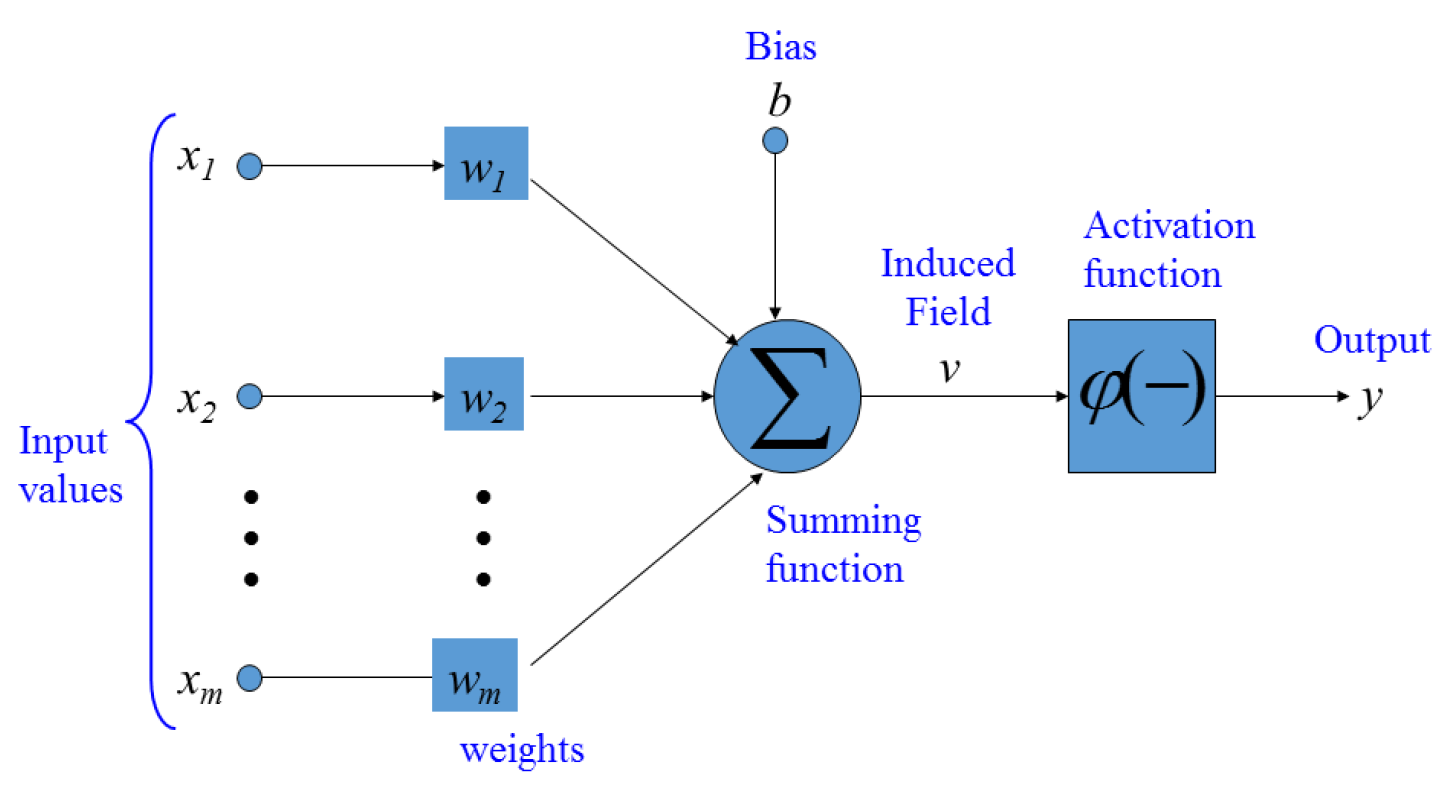
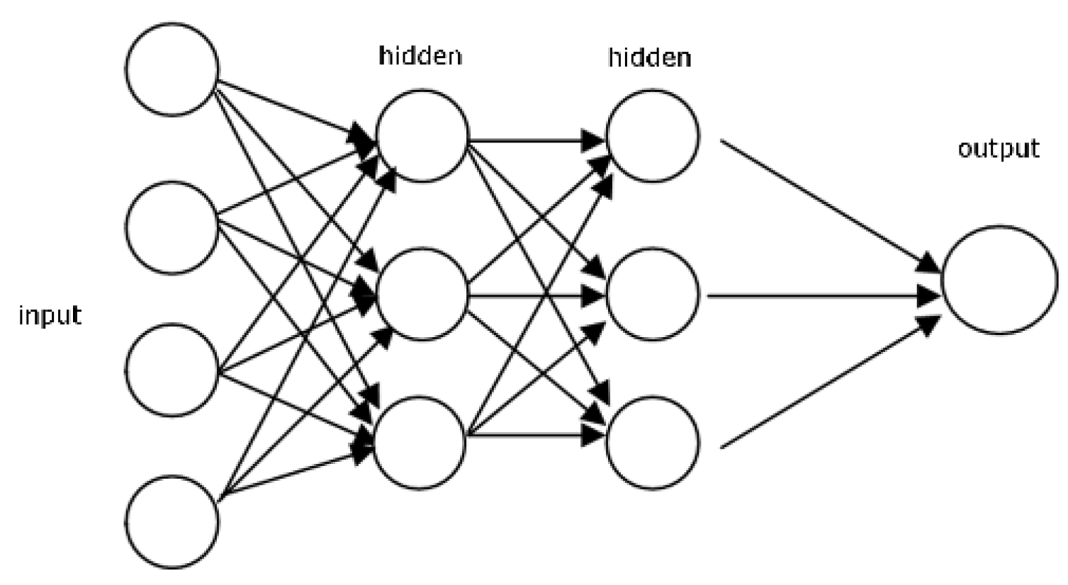
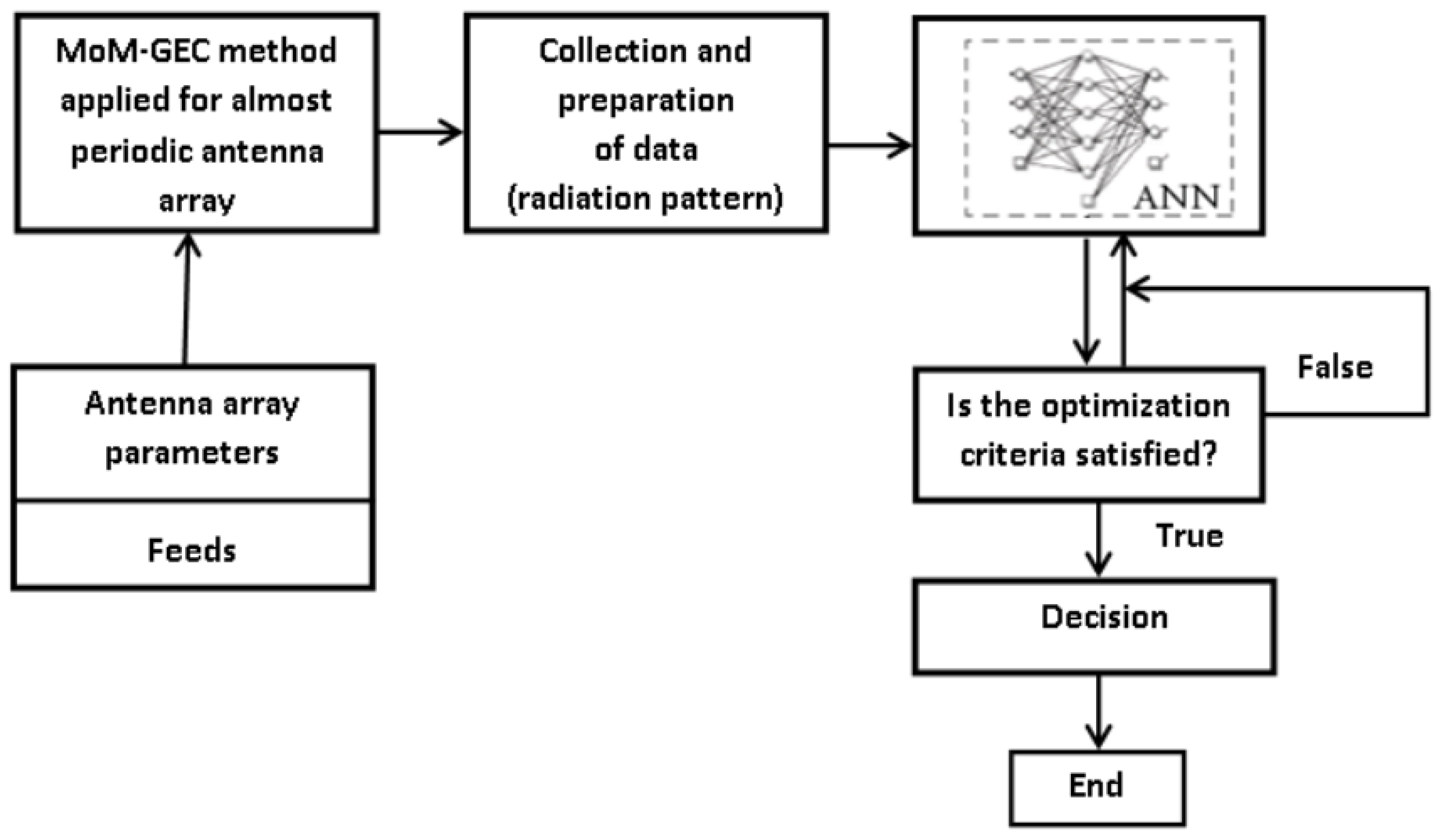
3. Concept of Artificial Neural Networks (ANNs)

As shown in our previous work, this section explains how to conjoin artificial neural networks and almost periodic antenna array systems [14,45,46].

A neural network is a way to model any input to an output by establishing connections between their related radiation model data, especially if nothing is known about the model. In fact, the neural network technique is commonly used in two stages: the training phase and the performance phase. For more precision, the MLP network architecture structure is fixed: the number of hidden layers and neurons (nodes) in each layer. The activation functions of each layer are also chosen at this stage—i.e., they are supposed to be known. The unknown parameters to be estimated are the weights and biases. Many algorithms exist to define the network parameters. Here, we will focus only on the use of the Levenberg–Marquardt method, which is generally more efficient than other algorithms but requires more memory than most [15,16,47,48,49,50,51]. We briefly summarize the learning algorithm procedure for multilayer perceptron networks:

1.

The structure of the network is first defined. In the network, activation functions are chosen and the network parameters, weights, and biases are initialized.

2.

The parameters associated with the training algorithm—the error goal, the maximum number of epochs (iterations), etc.—are defined.

3.

The training algorithm is called.

4.

Once the neural network is determined, the result is first tested by simulating the output of the neural network with the measured input data. This result is compared to the measured output. The final validation must be performed with independent data.

In general, three different types of dataset (input) are employed, known as the training set, validation set, and test set. The training set is a set of values that hold information about the target function for training the network. The validation set is assigned to the early stopping technique. During the training phase, the validation error is monitored to prevent the network from overfitting the training data. Normally, the test set is just used to assess the performance of the network afterward. Ordinarily, 60% of the data are used for training the network and the remaining 40% are used equally for validating and testing the network on unlearned inputs [13,45]. Specifically, MATLAB (commonly used) randomly divides the input vectors and target vectors into three known sets.

• Sixty percent are used for training.
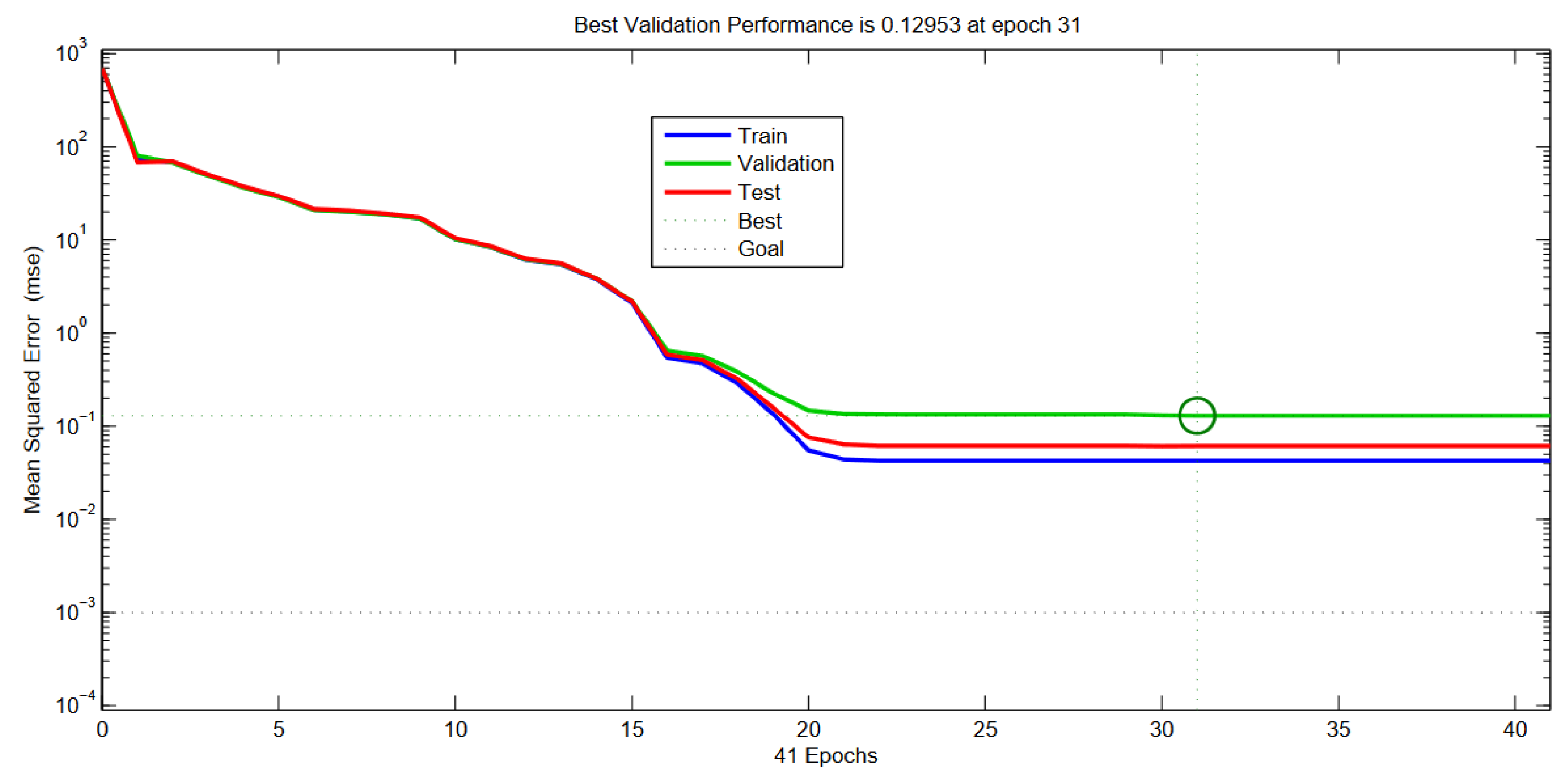
• Twenty percent are used to validate that the network is generalizing and to stop training before overfitting.
• The last 20% are used for a completely independent test of network generalization.

The structure of an ANN is provided in Figure 3 and Figure 4, when the learning phase allowed to elaborate the synaptic weights taken from each formal neuron. In this example, we are using a feed-forward network with a default tan-sigmoid transfer function in the hidden layer and a linear transfer function in the output layer.

Table 1. ANN training parameters [21,31].

Number of input neurons	100
Number of hidden layers	2
Number of output neurons	1
Algorithm	lm
Learning rate	0.01
Momentum	0.95
MSE goal	$1\times {10}^{-3}$
Minimum performance gradient	$1\times {10}^{-5}$
Initial mu	0.001
mu decrease factor	0.1
mu increase factor	10
Maximum mu	$1\times {10}^{10}$
Epochs between displays	25
Generate command-line output	false
Show training GUI	true
Maximum time to train in seconds	inf
Maximum number of epochs	300
Regularization parameter	0.8
Transfer function in hidden layer	tan-sigmoid (“tansig”)
Transfer function in output layer	linear(“purelin”)

lists the training parameters of our artificial neural network (ANN) and the architectural parameters prepared for the implementation of the ANN models [13,45].

After the training phase, the performance phases of the almost periodic array were performed to obtain the optimal weights for the new incoming signals. The performance analysis of this application can be examined by changing the number of antenna elements, the radiation value, the target applications and the angular separation between the incoming signals [15,16].

In this work, the Levenberg–Marquardt minimization algorithm (LMA) was used to train the ANN. The accuracy of its models was evaluated by the mean sum of squared error (MSE) between the calculated (desired) radiation pattern obtained using numerical analysis and the predicted values for the training dataset [15]. We executed a linear regression between the network outputs and the corresponding targets [50].

4. Results and Observations

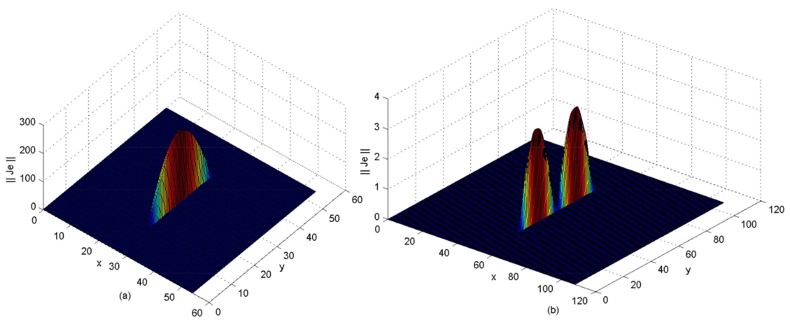
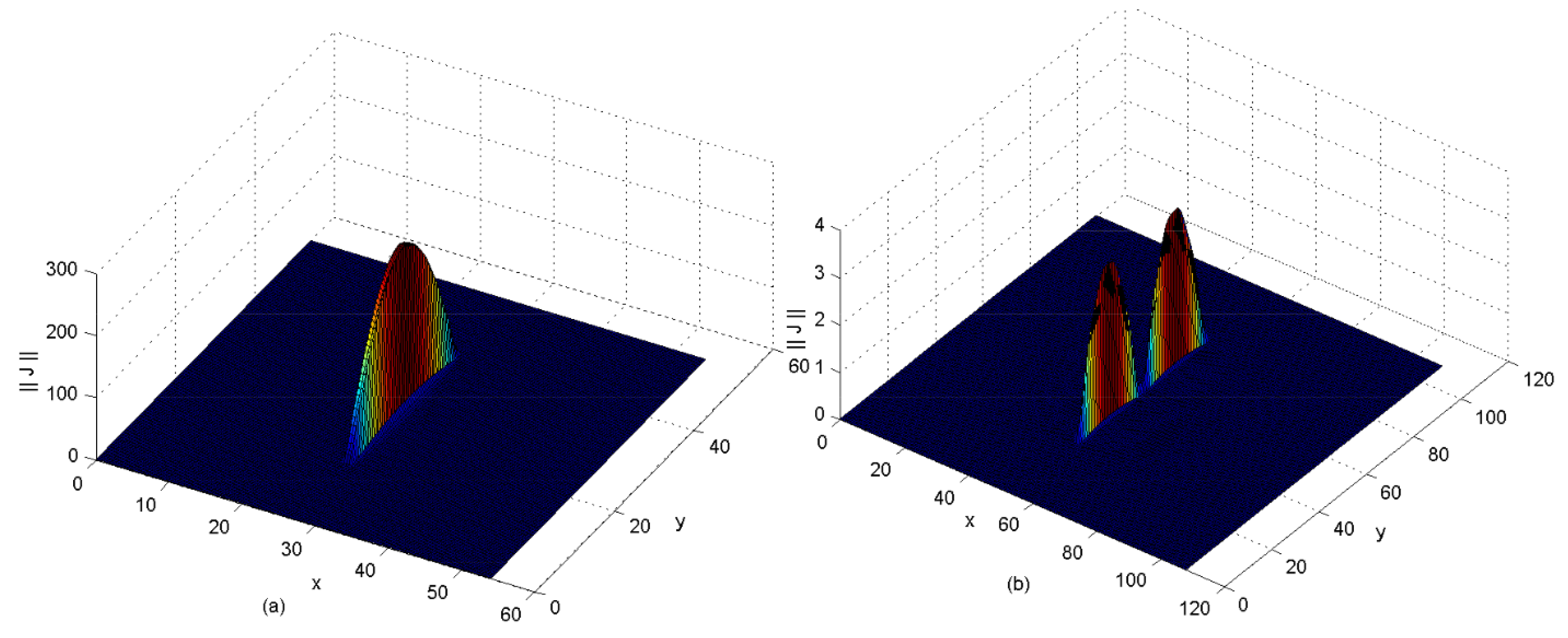
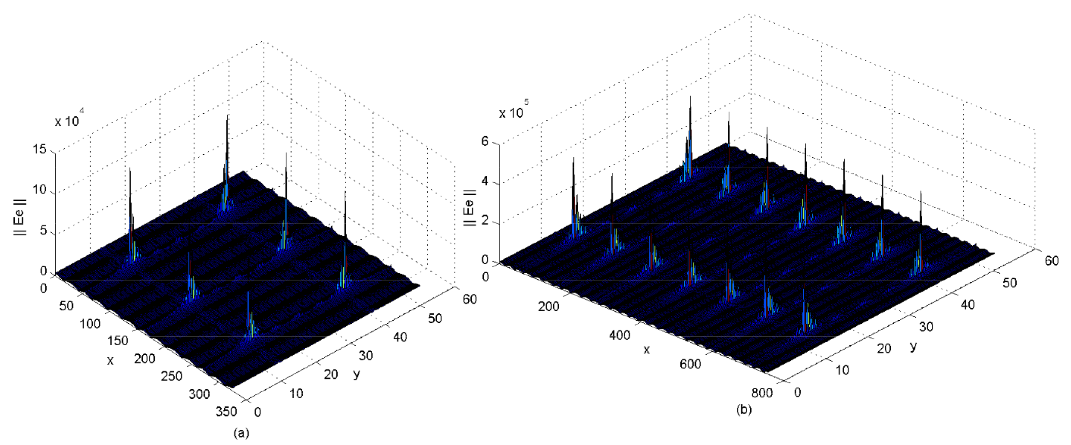
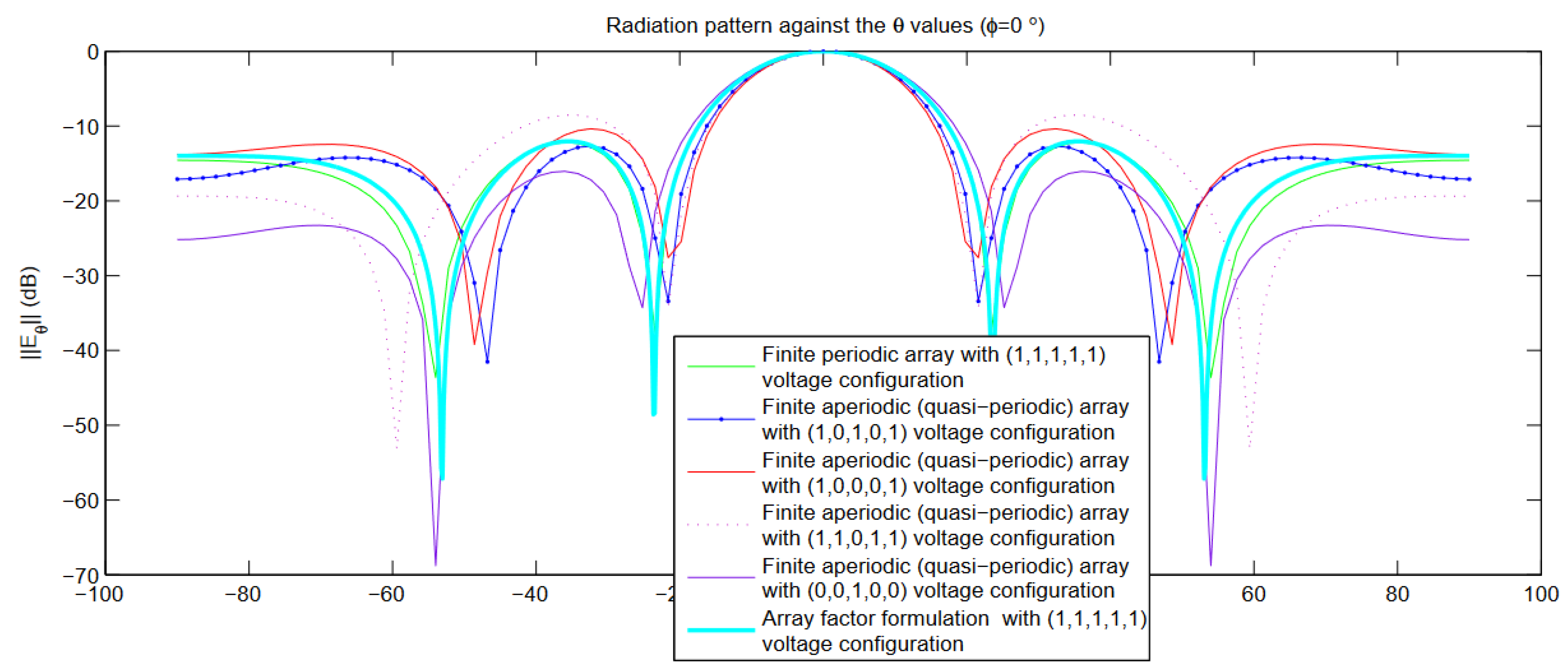
4.1. Numerical Results

In previous work, we studied the convergence level of the input impedance and the current distributions as functions of the guide’s modes and the trial functions, to demonstrate the coupling terms of the almost periodic array [2,3]. This study focused essentially on creating the radiation pattern associated with the planar almost periodic structures [37,38,39]. First, the electromagnetic states in electric and current fields of the proposed configuration examples must be taken, which are present at the waveguide aperture. Then, the desired radiation pattern (or the electric far-field) can be computed using the main Fourier expression written and explained in the previous Section [4,37,38,39], where the near field distribution defined on the discontinuity plane is weighted by a numerical MoM-GEC formulation [2,3,5]. To validate the structure, a comparison curve between the MoM-GEC and HFSS tool is presented in terms of input impedance, as shown in Figure 5.

Figure 6, Figure 7 and Figure 8 illustrate numerical current densities and their corresponding electric fields that were calculated for a unit cell of a periodic planar dipole antenna surrounded by periodic walls. As a result, the far-field of the given unit structure can be described by Figure 9 [2,3,4,5,52].

In this way, the preceding case of the basic element should be generalized to an almost periodic array configuration [2,3,37,38,39]. Thus, based on the formulation problem detailed in [2,3], the electromagnetic fields (E, J) of the whole structure can be shown. Thus, Figure 10, Figure 11 and Figure 12 allow one to verify all the proposed boundary conditions in terms of current and electric fields associated with the periodic planar structure.

Identically, the 1D and 2D quasi-periodic structures will follow the same pattern when representing the current and electric fields, as indicated in Figure 13, Figure 14, Figure 15, Figure 16 and Figure 17. It is shown that the electromagnetic coupling is expressed by the lying of a weak current surface on the non-exciting elements of the aperiodic configuration (which explains also the phenomenon of leaky waves). As shown in Figure 14, a Gibbs effect appears when the guide’s modes number has not correctly reached the convergence level.

In the same way, the radiating pattern of the whole planar almost periodic dipole antenna array can be given by Figure 18, Figure 19 and Figure 20. The mutual coupling effects are taken into account by varying the separation periods and the number of elements when the electromagnetic calculation is achieved, as illustrated by the same figures.

According to Figure 18 and Figure 19, the proposed structure offers high directivity with a reduced main radiation beam, but suffers from a high sidelobe level (SLL), especially when the number of elements is high and the array elements are decoupled (has a separation period ($d_x\gg \lambda$). The good radiation pattern description was obtained in both E-plane and H-plane cuts at the operative frequency f = $5.4$ GHz, as shown in Figure 20.

A good comparison was achieved between periodic and aperiodic structures in terms of the radiation pattern, as given in Figure 21. To validate the latter result, an array factor formulation was proposed, which is applicable for a periodic array containing isotropic elements with separation $d_x\ge \frac{\lambda }{2}$.

Figure 22 shows the radiation beam steering (with ${\varphi }_s=0^{\circ },{\theta }_s={45}^{\circ }$) of different periodic and aperiodic arrays, and explains how to reduce side lobe levels by varying the voltage configurations. As shown, the proposed antenna structures have a good beam steering property, which is highly effective at the spherical beam coverage.

In Figure 23, representations of the electric field at the waveguide aperture (the discontinuity plane) are shown for different cases of electric and periodic walls, and compared to the HFSS software results, which show different magnitudes of electric field (by checking boundary conditions). Figure 24 and Figure 25 show the resulting radiation patterns for the cases in Figure 23. The same shape of the main lobe is visualized (differences detailed in Figure 24). Differences are due to the weight of the electric field defined at the guide aperture in each case shown in Figure 23. As well, Figure 26 shows validation of the radiation pattern (in the main direction ${\theta }_s=0°$) obtained with MoM-GEC and HFSS tools for a coupled antenna array of five elements and a period equal to 27 mm (≈$\frac{{\lambda }_0}{2}$). The main lobe has the same shape, but our method produced a more accurate sidelobe (very poor with HFSS). The use of HFSS soft for scanning and covering the space around the antenna system is possible; however, our method is more flexible for electronic scanning [47,53].

4.2. ANN Application

The diagram presented in Figure 27 describes the rest of the process of generating the optimized radiation pattern. Firstly, the necessary data collection for training was performed by employing a numerical calculation of the moment method combined with an equivalent circuit, using the parameters of the almost periodic array structure already given. Then, the architectural parameters of the default ANN model were established, and a comprehensive analysis of the ANN’s training was carried out in order to develop a predictive performance. To propose an optimal ANN representation with high performance and to improve the generalization capabilities of the ANN models, the early stopping (ES) method was mainly used in ANN training [34].

In general, two frequently used ways to overcome the overtraining condition, i.e., to decide when to terminate the training process, are the early stopping (ES) and regularization methods. Early stopping (ES) is typically used because it is easy to be understood and implemented and has outperformed the regularization methods. In order to utilize the ES method, the existing data must be divided into three sets [13]:

1.

The training set was used to determine ANN weights.

2.

The validation set was used to check the ANN’s performance and decide when to stop the training process.

3.

The test set was used to assess the performance capabilities of the developed ANN model.

A more detailed explanation of the ES method is illustrated graphically in Figure 28, Figure 29 and Figure 30. The methodology of the ES approach can be found in [13,34].

As seen in Figure 29 and Figure 30, a good accuracy improvement in the generalization of the normalized radiation field was proven with the early stopping (es) technique. However, an ANN based on the ES method (network with early stopping) was able to generate the results of the synthesis very quickly compared to the default artificial neural network (network without early stopping) which required much more CPU time and memory. In consequence, the network with the ES method could better adapt to the test dataset with fewer divergences, so the early stopping feature can be used to prevent the over adaptation of the network towards the training data.

To obtain the computation time acceleration, the difference in computation time between the default training and training with the early stopping method (using the Levenberg algorithm) is given in

Table 2. Time consumption of learning for artificial neural networks with and without early stopping.

Training	Time Consumed by the Algorithm (s)
Default training (with levenberg algorithm)	$126.863$
Training with early stopping method (using levenberg algorithm)	$19.276$

. It shows that the time consumption of the early stopping method was less than the time required for the default method (without early stopping).

Due to the results in

Table 3. Total CPU time (in seconds) used by electromagnetic calculation optimized through an ANN algorithm.

EM Calculation Using ANN Optimization	ANN with Spatial MoM Coding	ANN with Floquet MoM Coding
Elapsed CPU Time (in seconds)	$2704.502344$	$1750.368348$

, the optimization and synthesis using ANN with the Floquet moment method [2,3,4] was superior to the ANN with the spatial method, when the motifs were considered coupled, because of the CPU time of the modal analysis was more efficient and short compared to the old spatial MoM.

As the elapsed CPU time, the used memory is proven and discussed in our previous work, where the modal Floquet analysis remains more appreciated in comparison to the classical spatial MoM [2,3,4].

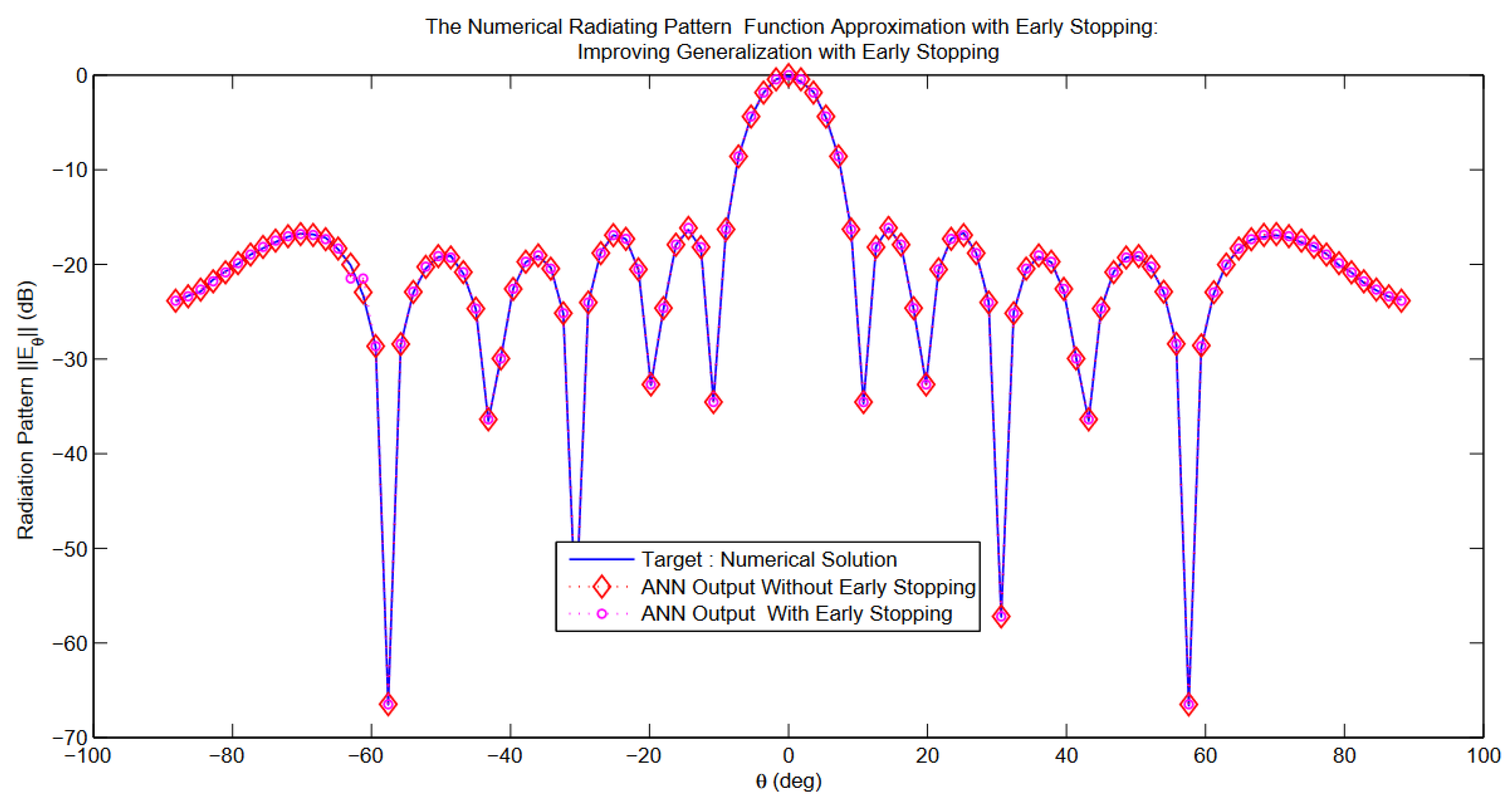
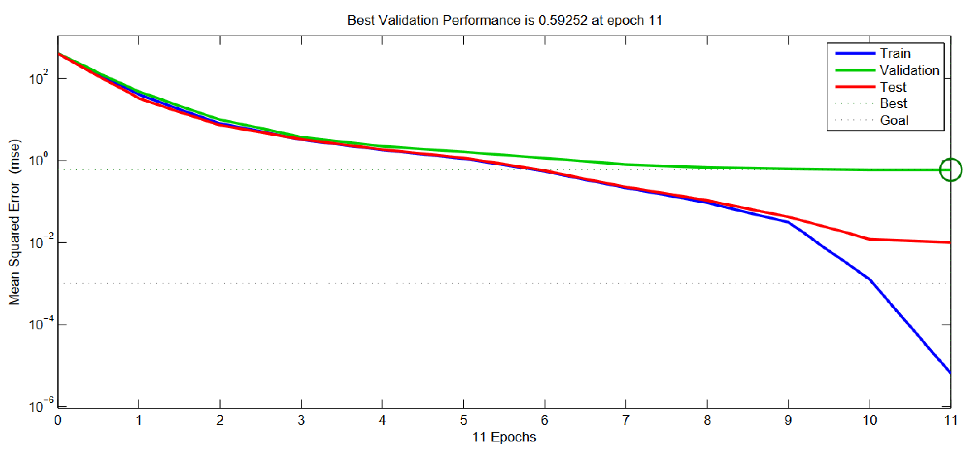
4.3. ANN Performance

When the training process and the application of the multilayer neural network were complete, the network’s performance was checked to determine if any changes needed to be implemented in the training algorithm, the network architecture, or the datasets. We measured the network’s performance according to the mean of squared errors. The accuracy of the ANN models was evaluated by the mean sum of squared error (MSE) between the target and output values using the training dataset [30]. A plot of the training errors is shown in Figure 31. The mean squared error of the aperiodic configuration is presented in Figure 32. This training was stopped when the training error decreased with convergence to the optimal solution. As is clear, the training process for the ANN model was concluded at 31 training epochs when the MSE reached the value of 0.12953 (for the aperiodic structure, the MSE was 0.59252 at 11 training epochs). The early stopping technique was employed when 11 validation checks were failed before epoch 40; the maximum gradient descent value was 0.27225. (The gradient decent value of the aperiodic structure was 0.0475 when 11 validation checks were failed at epoch 11). A reasonable Mu value of 1.00 was reached, which would cause convergence of the network rapidly, as presented in the overall progress of the ANN [13,15,16].

The next validation step in the network was to create a regression plot showing the relationship between the outputs of the network and the targets. If training is perfect, the network outputs and the targets match, but the relationship is rarely perfect in practice. The dotted line in the training graph represents the perfect result: outputs = targets. The solid line indicates the best-fit linear regression line between the outputs and the targets. The R-value is an indication of the relationship between the outputs and the objectives. If R = 1, this indicates that there is an exact linear relationship between outputs and targets. If R is close to zero, there is no linear relationship between outputs and targets. In this example, the training data have a good fit. Regression analysis was performed with the ANN model when the network finished training. It is a statistical process for estimating the relationships between the outputs and targets of a network. The regression function takes two parameters’ values (targets, outputs) and plots the linear relationship. According to all the graphs in Figure 33 (in the same manner for the aperiodic antenna array), the best regression result for the validation was R = 0.99993 (concerning the aperiodic array, R = 0.9958), that for the testing data was R = 0.99996 (for the aperiodic array, R = 0.99993), and that for the training data was R = 1. The overall regression value was R = 0.99996 (for the aperiodic array, R = 0.99857). This proves the developed model and the network procedure of training, testing and validation are significantly valid [50].

5. Conclusions

We aimed to synthesize the radiation pattern of planar almost periodic arrays, including the mutual coupling effects, which were modeled by the known moment method combined with a generalized equivalent circuit (MoM-GEC). We used a novel ANN as a computational model to create the array pattern.

Many advantages were shown for synthesizing the numerical radiation pattern using an artificial neural network. For example:

• Reduced computational time and memory usage, especially when adopting the early stopping method, which eliminates the overfitting problem.
• It is suitable for use with a coupled and complex quasi-periodic configuration.
• It is simple and easier to use than other optimization techniques (genetic, LMS, etc.).
• It is adaptable to complex electromagnetic calculations taking into account the effects of mutual coupling.

This analysis will be the basis for future work on neural network solutions for the synthesis of non-uniform, irregular, and sparse antenna arrays.

In future research, we suggest using other optimization techniques (genetic, LMS, etc.) for modeling complex almost periodic arrays to predict the desired radiation that can be adopted to increase the gain and to scan the range by suppressing the sidelobe level (SLL).

References

1. Vardaxoglou, J.C. Frequency Selective Surfaces, Analysis and Design; John Wiley and Sons: Hoboken, NJ, USA, 1997. [Google Scholar]
2. Hamdi, B.; Aguili, T.; Raveu, N.; Baudrand, H. Calculation of the mutual coupling parameters and their effects in 1-D planar almost periodic structures. Prog. Electromagn. Res. B 2014, 59, 269–289. [Google Scholar] [CrossRef] [Green Version]
3. Hamdi, B.; Aguili, T.; Baudrand, H. Floquet modal analysis to modelize and study 2-D planar almost periodic structures in finite and infinite extent with coupled motifs. Prog. Electromagn. Res. B 2015, 62, 63–86. [Google Scholar] [CrossRef] [Green Version]
4. Mekkioui, Z.; Baudrand, H. Bi-dimensional bi-periodic centred-fed microstrip leaky-wave antenna analysis by a source modal decomposition in spectral domain. IET Microw. Antennas Propag. 2009, 3, 1141–1149. [Google Scholar] [CrossRef]
5. Hamdi, B.; Aguili, T.; Baudrand, H. Uni-dimensional planar almost periodic structures analysis to decompose central arbitrary located source in spectral domain. In Proceedings of the 2012 15 International Symposium on Antenna Technology and Applied Electromagnetics (ANTEM), Toulouse, France, 25–28 June 2012; pp. 1–5. [Google Scholar]
6. Sagar, M.S.I.; Ouassal, H.; Omi, A.I.; Wisniewska, A.; Jalajamony, H.M.; Fernandez, R.E.; Sekhar, P.K. Application of Machine Learning in Electromagnetics: Mini-Review. Electronics 2021, 10, 2752. [Google Scholar] [CrossRef]
7. Taghvaee, H. On Scalable, Reconfigurable, and Intelligent Metasurfaces; Universitat Politècnica de Catalunya: Barcelona, Spain, 2021. [Google Scholar]
8. Laseetha, T.J.; Sukanesh, R. Synthesis of uniform linear antenna array using genetic algorithm with cost based roulette to maximize sidelobe level reduction. Int. J. Inf. Acquis. 2011, 8, 171–179. [Google Scholar] [CrossRef]
9. Brown, A.D. (Ed.) Electronically Scanned Arrays MATLAB® Modeling and Simulation; CRC Press: Boca Raton, FL, USA, 2017. [Google Scholar]
10. Babale, S.A.; Dajab, D.D.; Ahmad, K. Synthesis of a Linear Antenna Array for Maximum Side-lobe Level Reduction. Int. J. Comput. Appl. 2014, 85, 24–28. [Google Scholar]
11. Singh, A.; Singh, S. Design and optimization of a modified Sierpinski fractal antenna for broadband applications. Appl. Soft Comput. 2016, 38, 843–850. [Google Scholar] [CrossRef]
12. Yan, K.K.; Lu, Y. Sidelobe reduction in array-pattern synthesis using genetic algorithm. IEEE Trans. Antennas Propag. 1997, 45, 1117–1122. [Google Scholar]
13. Hamdi, B.; Limam, S.; Aguili, T. Uniform and concentric circular antenna arrays synthesis for smart antenna systems using artificial neural network algorithm. Prog. Electromagn. Res. B 2016, 67, 91–105. [Google Scholar] [CrossRef] [Green Version]
14. Freni, A.; Mussetta, M.; Pirinoli, P. Neural network characterization of reflectarray antennas. Int. J. Antennas Propag. 2012, 2012, 541354. [Google Scholar] [CrossRef]
15. Merad, L.; Bendimerad, F.T.; Meriah, S.M.; Djennas, S.A. Neural networks for synthesis and optimization of antenna arrays. Radioengineering 2007, 16, 23–30. [Google Scholar]
16. Ghayoula, R.; Fadlallah, N.; Gharsallah, A.; Rammal, M. Phase-only adaptive nulling with neural networks for antenna array synthesis. IET Microw. Antennas Propag. 2009, 3, 154–163. [Google Scholar] [CrossRef]
17. Oueslati, A.; Menudier, C.; Thevenot, M.; Monediere, T. Potentialities of hybrid arrays with parasitic elements. In Proceedings of the 8th European Conference on Antennas and Propagation (EuCAP 2014), The Hague, The Netherlands, 6–11 April 2014; pp. 1829–1830. [Google Scholar]
18. Abdallah, Y.; Menudier, C.; Thevenot, M.; Monediere, T. Investigations of the effects of mutual coupling in reflectarray antennas. IEEE Antennas Propag. Mag. 2013, 55, 49–61. [Google Scholar] [CrossRef]
19. Wei, W.Y.; Shi, Y.; Yang, J.X.; Meng, H.X. Artificial neural network and convex optimization enable antenna array design. Int. J. Microw. Comput.-Aided Eng. 2021, 31, e22593. [Google Scholar] [CrossRef]
20. Cui, C.; Li, W.T.; Ye, X.T.; Rocca, P.; Hei, Y.Q.; Shi, X.W. An Effective Artificial Neural Network-Based Method for Linear Array Beampattern Synthesis. IEEE Trans. Antennas Propag. 2021, 69, 6431–6443. [Google Scholar] [CrossRef]
21. Patnaik, A.; Choudhury, B.; Pradhan, P.; Mishra, R.K.; Christodoulou, C. An ANN application for fault finding in antenna arrays. IEEE Trans. Antennas Propag. 2007, 55, 775–777. [Google Scholar] [CrossRef]
22. Ozdemir, E.; Akgol, O.; Ozkan Alkurt, F.; Karaaslan, M.; Abdulkarim, Y.I.; Deng, L. Mutual Coupling Reduction of Cross-Dipole Antenna for Base Stations by Using a Neural Network Approach. Appl. Sci. 2020, 10, 378. [Google Scholar] [CrossRef] [Green Version]
23. Taghvaee, H.; Jain, A.; Timoneda, X.; Liaskos, C.; Abadal, S.; Alarcón, E.; Cabellos-Aparicio, A. Radiation Pattern Prediction for Metasurfaces: A Neural Network-Based Approach. Sensors 2021, 21, 2765. [Google Scholar] [CrossRef]
24. Reddy, B.; Vakula, D.; Sarma, N.V.S.N. Design of multiple function antenna array using radial basis function neural network. J. Microw. Optoelectron. Electromagn. Appl. 2013, 12, 210–216. [Google Scholar] [CrossRef]
25. Wang, Z.; Fang, S. ANN synthesis model of single-feed corner-truncated circularly polarized microstrip antenna with an air gap for wideband applications. Int. J. Antennas Propag. 2014, 2014, 392843. [Google Scholar] [CrossRef] [Green Version]
26. Famoriji, O.J.; Shongwe, T. Electromagnetic machine learning for estimation and mitigation of mutual coupling in strongly coupled arrays. ICT Express 2021. [Google Scholar] [CrossRef]
27. Dukare, M.P.; Badjate, S. Modeling Of Antenna Array Parameter Using Neural Network For Directivity Prediction. Int. J. Adv. Res. Electron. Commun. Eng. 2015, 4, 1946–1950. [Google Scholar]
28. Rahnamai, K.; Arabshahi, P.; Yan, T.Y.; Pham, T.; Finley, S.G. An Intelligent Fault Detection and Isolation Architecture for Antenna Arrays. The Telecommunications and Data Acquisition Progress Report 42-132. 1998. Available online: https://ipnpr.jpl.nasa.gov/progress_report/42-132/132A.pdf (accessed on 3 January 2022).
29. Kurup, D.G. Active and Passive Unequally Spaced Reflect-Arrays and Elements of RF Integration Techniques. Doctoral Dissertation, Acta Universitatis Upsaliensis, Uppsala, Sweden, 2003. [Google Scholar]
30. Sallomi, A.H.; Ahmed, S. Elman recurrent neural network application in adaptive beamforming of smart antenna system. Int. J. Comput. Appl. 2015, 975, 8887. [Google Scholar]
31. Xin, W.; Konno, K.; Chen, Q. Applying Artificial Neural Network to Diagnose Array Antennas. 2019. Available online: http://www.chenq.ecei.tohoku.ac.jp/common/item/pdf/densou/2019Feb_wangxin.pdf (accessed on 3 January 2022).
32. Ghayoula, R.; Fadlallah, N.; Gharsallah, A.; Rammal, M. Design, modelling, and synthesis of radiation pattern of intelligent antenna by artificial neural networks. Appl. Comput. Electromagn. Soc. J. 2008, 23, 336–344. [Google Scholar]
33. Kumar, U.; Kapoor, R. Patch Antenna Array Fault Modeling and its Monitoring. IOSR J. Electron. Commun. Eng. 2012, 6, 6–11. [Google Scholar] [CrossRef]
34. Wang, L.; Quek, H.C.; Tee, K.H.; Zhou, N.; Wan, C. Optimal size of a feedforward neural network: How much does it matter? In Proceedings of the Joint International Conference on Autonomic and Autonomous Systems and International Conference on Networking and Services-(icas-isns’ 05), Papeete, France, 23–28 October 2005; p. 69. [Google Scholar]
35. Thevenot, M.; Menudier, C.; El Sayed Ahmad, A.; Zakka El Nashef, G.; Fezai, F.; Abdallah, Y.; Monediere, T. Synthesis of antenna arrays and parasitic antenna arrays with mutual couplings. Int. J. Antennas Propag. 2012, 2012, 309728. [Google Scholar] [CrossRef] [Green Version]
36. Valerio, G.; Baccarelli, P.; Burghignoli, P.; Galli, A.; Rodríguez-Berral, R.; Mesa, F. Analysis of periodic shielded microstrip lines excited by nonperiodic sources through the array scanning method. Radio Sci. 2008, 43, 1–15. [Google Scholar] [CrossRef]
37. Mekkioui, Z.; Baudrand, H. A full-wave analysis of uniform microstrip leaky-wave antenna with arbitrary metallic strips. Electromagnetics 2008, 28, 296–314. [Google Scholar] [CrossRef]
38. Mekkioui, Z.; Baudrand, H. Effects of multilayers superstrates on microstrip leaky-wave antennas radiating characteristics and performances. Electromagnetics 2005, 25, 133–151. [Google Scholar] [CrossRef]
39. Mekkioui, Z.; Baudrand, H. Analyse rigoureuse d’antenne diélectrique microruban uniforme à ondes de fuite. In Annales des Télécommunications; Springer: Berlin/Heidelberg, Germany, 2002; Volume 57, pp. 540–560. [Google Scholar]
40. Aidi, M.; Hajji, M.; Ben Ammar, A.; Aguili, T. Graphene nanoribbon antenna modeling based on MoM-GEC method for electromagnetic nanocommunications in the terahertz range. J. Electromagn. Waves Appl. 2016, 30, 1032–1048. [Google Scholar] [CrossRef]
41. Yann, C. Modélisation électromagnétique de cellules actives environnées-Application à l’analyse et la synthèse d’une antenne reflectarray à balayage électronique. Doctoral Dissertation, INSA de Rennes, Rennes, France, 2012. [Google Scholar]
42. Tchikaya, E.B. Modélisation électromagnétique des Surfaces Sélectives en Fréquence finies uniformes et non-uniformes par la Technique de Changement d’Echelle (SCT). Doctoral Dissertation, Polytechnique Toulouse, Toulouse, France, 2010. [Google Scholar]
43. Costa, B.F.; Abrao, T. Closed-form directivity expression for arbitrary volumetric antenna arrays. IEEE Trans. Antennas Propag. 2018, 66, 7443–7448. [Google Scholar] [CrossRef]
44. Bilel, H.; Taoufik, A. Floquet Spectral Almost-Periodic Modulation of Massive Finite and Infinite Strongly Coupled Arrays: Dense-Massive-MIMO, Intelligent-Surfaces, 5G, and 6G Applications. Electronics 2022, 11, 36. [Google Scholar] [CrossRef]
45. Bilel, H.; Selma, L.; Taoufik, A. Artificial neural network (ANN) approach for synthesis and optimization of (3D) three-dimensional periodic phased array antenna. In Proceedings of the 2016 17th International Symposium on Antenna Technology and Applied Electromagnetics (ANTEM), Montreal, QC, Canada, 10–13 July 2016; pp. 1–6. [Google Scholar]
46. Dudczyk, J.; Kawalec, A. Adaptive forming of the beam pattern of microstrip antenna with the use of an artificial neural network. Int. J. Antennas Propag. 2012, 2012, 935073. [Google Scholar] [CrossRef]
47. Hamdi, B.; Nouainia, A.; Aguili, T.; Baudrand, H. ANN Synthesis and Optimization of Electronically Scanned Coupled Planar Periodic and Aperiodic Antenna Arrays Modeled by the MoM-GEC Approach. In Proceedings of the 2020 IEEE Eighth International Conference on Communications and Electronics (ICCE)—MICROWAVE ENGINEERING, Phu Quoc Island, Vietnam, 13–15 January 2021; Available online: https://vixra.org/pdf/2111.0161v1.pdf (accessed on 3 January 2022).
48. Kapetanakis, T.N.; Vardiambasis, I.O.; Liodakis, G.S.; Ioannidou, M.P.; Maras, A.M. Smart antenna design using neural networks. In Proceedings of the 8th International Conference: New Horizons in Industry, Business and Education (NHIBE 2013), Chania, Greece, 29 August 2013; pp. 130–135. [Google Scholar]
49. Rawat, A.; Yadav, R.N.; Shrivastava, S.C. Neural network applications in smart antenna arrays: A review. AEU-Int. J. Electron. Commun. 2012, 66, 903–912. [Google Scholar] [CrossRef]
50. Ali, B.A.; Salit, M.S.; Zainudin, E.S.; Othman, M. Integration of artificial neural network and expert system for material classification of natural fibre reinforced polymer composites. Am. J. Appl. Sci. 2015, 12, 174. [Google Scholar]
51. Ghayoula, E.; Ghayoula, R.; Haj-Taieb, M.; Chouinard, J.Y.; Bouallegue, A. Pattern Synthesis Using Hybrid Fourier-Neural Networks for IEEE 802.11 MIMO Application. Prog. Electromagn. Res. B 2016, 67, 45–58. [Google Scholar] [CrossRef] [Green Version]
52. Ayari, M.; Aguili, T.; Temimi, H.; Baudrand, H. An extended version of Transverse Wave Approach (TWA) for full-wave investigation of planar structures. J. Microw. Optoelectron. Electromagn. Appl. (JMOe) 2008, 7, 123–138. [Google Scholar]
53. Hamdi, B.; Aguili, T. MoM-GEC combined with Floquet analysis to study scanned coupled almost periodic antenna arrays in massive MIMO for 5G generation and FMCW automotive radar applications. In Proceedings of the 2020 IEEE International Symposium on Antennas and Propagation and North American Radio Science Meeting, Montreal, QC, Canada, 5–10 July 2020; pp. 1941–1942. [Google Scholar]
54. 14.1 Project:Midpoint Sums Approximating Double Integrals (Using MATLAB). Available online: https://people.math.aau.dk/~olav/undervisning/ide10/proj14-1.pdf (accessed on 3 January 2022).
55. Das, S.K. Antenna and Wave Propagation; Tata McGraw-Hill Education: New York, NY, USA, 2013. [Google Scholar]
Figure 1. Diagram of periodic planar phased array dipoles: the walls of the environment can be selected from EEEE (waveguide with electric walls), EMEM (waveguide with two electric walls and two magnetic walls), EPEP (waveguide with two electric walls and two periodic walls), and PPPP (waveguide with periodic walls).
Electronics 11 00703 g001
Figure 2. Section of periodic phased array microstrip lines (planar dipoles): unit cell delimited by periodic walls.
Electronics 11 00703 g002
Figure 3. Basic structure of an artificial neuron.
Electronics 11 00703 g003
Figure 4. An illustration of a typical feedforward network.
Electronics 11 00703 g004
Figure 5. Validation of the evaluated input impedance obtained by the MoM-GEC and the HFSS tool for a unit cell of a dipole: α 0 = 0 rad m 1 , β 0 = 0 rad m 1 , w = 1 mm , δ = 0.75 mm ( w λ 0 , δ λ 0 ) , d x = 108 mm , d y = 108 mm , L = λ 0 54 mm (at the fixed frequency f = 5.4 GHz ) , h = 1.25 mm, and ϵ = ϵ r = 1 (air).
Electronics 11 00703 g005
Figure 6. Current density for a unit cell of an almost periodic 2D array (half-wave and full-wave dipoles) defined over the guide aperture, described by the test functions using: f = 5.4 GHz, α 0 = 0 rad m 1 , β 0 = 0 rad m 1 , w = 1 mm, δ = 0.75 mm ( w λ 0 , δ λ 0 ) , d x = 108 mm, and d y = 108 mm. (a) L = λ 0 2 27 mm; (b) L = λ 0 54 mm, h = 1.25 mm and ϵ = ϵ r = 1 (air) (see [1] for a comparison).
Electronics 11 00703 g006
Figure 7. Current density for a unit cell of 2D almost periodic array (half and full wave dipoles) defined by the guide wave’s aperture, described by the basis functions (guide’s modes) using: f = 5.4 GHz, α 0 = 0 rad m 1 , β 0 = 0 rad m 1 , w = 1 mm, δ = 0.75 mm ( w λ 0 , δ λ 0 ) , d x = 108 mm, d y = 108 mm. (a) L = λ 0 2 27 mm; (b) L = λ 0 54 mm, h = 1.25 mm and ϵ = ϵ r = 1 (air) (see [1] for a comparison).
Electronics 11 00703 g007
Figure 8. Electric field of 2D almost periodic array’s unit cell (half and full wave dipoles) defined by the guide wave’s aperture, described by the basis functions (guide’s modes) using: f = 5.4 GHz, α 0 = 0 rad m 1 , β 0 = 0 rad m 1 , w = 1 mm , δ = 0.75 mm ( w λ 0 , δ λ 0 ) , d x = 108 mm , d y = 108 mm. (a) L = λ 0 2 27 mm; (b) L = λ 0 54 mm , h = 1.25 mm, and ϵ = ϵ r = 1 (air) (see [1] for a comparison).
Electronics 11 00703 g008
Figure 9. Radiation pattern calculated using the MoM-GEC method for a half-wave and full-wave dipole antenna: f = 5.4 GHz, α 0 = 0 rad m 1 , β 0 = 0 rad m 1 , w = 1 mm, δ = 0.75 mm ( w λ 0 , δ λ 0 ) , d x = 108 mm, d y = 108 mm. (Blue color) L = λ 0 2 27 mm; (Green color) L = λ 0 54 mm, h = 1.25 mm, and ϵ = ϵ r = 1 (air).
Electronics 11 00703 g009
Figure 10. Current density of an example of almost periodic 2D array (half-wave dipoles) defined by the guide wave aperture, described by (a) test functions or (b) basis functions (guide modes) at the operating frequency (f) of 5.4 GHz. The physical parameters used were: α 0 = 0 rad m 1 , β 0 = 0 rad m 1 , w = 1 mm, δ = 0.75 mm ( w λ 0 , δ λ 0 ) , d x = 108 mm, d y = 108 mm, L = λ 0 2 27 mm, h = 1.25 mm, and ϵ = ϵ r = 1 (air) (see [1] for a comparison).
Electronics 11 00703 g010
Figure 11. Current density of the almost periodic network (half-wave dipoles) defined on the aperture of the waveguide, described by (a) the test functions or (b) the basic functions (guide modes) at the operating frequency (f) of 5.4 GHz. The physical parameters used were: α 0 = 0 rad m 1 , β 0 = 0 rad m 1 , w = 1 mm, δ = 0.75 mm ( w λ 0 , δ λ 0 ) , d x = 108 mm, d y = 108 mm, L = λ 0 2 27 mm, h = 1.25 mm, and ϵ = ϵ r = 1 (air) (see [1] for a comparison).
Electronics 11 00703 g011
Figure 12. Electric field of the almost periodic array (half-wave dipoles) defined by the waveguide’s aperture, described by the basis functions (guide’s modes) using (a) three cells or (b) seven cells at the operating frequency (f) of 5.4 GHz. The physical parameters were: α 0 = 0 rad m 1 , β 0 = 0 rad m 1 , w = 1 mm, δ = 0.75 mm ( w λ 0 , δ λ 0 ) , d x = 108 mm, d y = 108 mm, L = λ 0 2 27 mm, h = 1.25 mm, and ϵ = ϵ r = 1 (air) (see [1] for a comparison).
Electronics 11 00703 g012
Figure 13. Current density of 1D aperiodic array’s example (half-wave dipoles) defined by the waveguide’s aperture, described by the test functions at the operating frequency (f) of 5.4 GHz. The physical parameters used were: α 0 = 0 rad m 1 , β 0 = 0 rad m 1 , w = 1 mm, δ = 0.75 mm ( w λ 0 , δ λ 0 ) , d x = 13.5 mm, d y = 108 mm, L = λ 0 2 27 mm, h = 1.25 mm, and ϵ = ϵ r = 1 (air).
Electronics 11 00703 g013
Figure 14. Current densities: examples of 1D aperiodic arrays (half-wave dipoles) that appeared on the guide wave’s aperture, described by the basis functions (Guide’s modes) (without convergence) at the operating frequency (f) of 5.4 GHz: (a) for an aperiodic exitation of type 10101, (b) for an aperiodic exitation type 10001. The physical parameters were: α 0 = 0 rad m 1 , β 0 = 0 rad m 1 , w = 1 mm, δ = 0.75 mm ( w λ 0 , δ λ 0 ) , d x = 27 mm, d y = 108 mm, L = λ 0 2 27 mm, h = 1.25 mm, and ϵ = ϵ r = 1 (air).
Electronics 11 00703 g014
Figure 15. Current densities: 1D and 2D of aperiodic array examples (half-wave dipoles) lying on the guide wave’s aperture and described by the basis functions (guide’s modes) at the operating frequency (f) of 5.4 GHz. The physical parameters were: α 0 = 0 rad m 1 , β 0 = 0 rad m 1 , w = 1 mm, δ = 0.75 mm ( w λ 0 , δ λ 0 ) , d x = 13.5 mm, d y = 108 mm, L = λ 0 2 27 mm, h = 1.25 mm, and ϵ = ϵ r = 1 (air).
Electronics 11 00703 g015
Figure 16. Distribution of the electric density for ( 5 × 1 ) aperiodic phased half-wavelength planar dipoles (with (1,0,1,0,1) voltage configuration) described with the basis functions (guide’s modes) at f = 5.4 GHz (using EEEE electric walls).
Electronics 11 00703 g016
Figure 17. Distribution of the electric density for ( 5 × 1 ) aperiodic phased half-wavelength planar dipoles (with (0,0,1,0,0) voltage configuration) described with the basis functions (guide’s modes) at f = 5.4 GHz (using EEEE electric walls).
Electronics 11 00703 g017
Figure 18. Radiation pattern computed with a MoM-GEC method against the motifs number at the operating frequency (f) of 5.4 GHz (periodic array).
Electronics 11 00703 g018
Figure 19. Radiation pattern computed with a MoM-GEC method against the periods at the operating frequency (f) of 5.4 GHz (periodic array).
Electronics 11 00703 g019
Figure 20. E-and H-plane cuts of the radiation pattern computed with a MoM-GEC method at the operating frequency (f) of 5.4 GHz (periodic array).
Electronics 11 00703 g020
Figure 21. Radiation patterns for distinct aperiodic configurations and periodic arrays using electromagnetic and analytic formulations (MoM-GEC and analytic formulations) [22].
Electronics 11 00703 g021
Figure 22. 3D Electronically scanned radiation pattern examples for distinct aperiodic array configurations compared to the periodic array obtained using the electromagnetic calculation (MoM-GEC method): ϕ s = 0 , θ s = 45 angles of steering: (a) An aperiodic configuration of type (0,0,1,0,0), (b) An aperiodic configuration of type (1,0,1,0,1), (c) A periodic configuration of type (1,1,1,1,1) [22].
Electronics 11 00703 g022
Figure 23. Electric field at the opening of a waveguide composed of 5 coupled planar dipoles (calculation provided by the MoM method and the HFSS software): d x λ 0 2 = 27 mm (period): (a) MoM-GEC with electric walls, (b) MoM-GEC with periodic walls, (c) HFSS Tool.
Electronics 11 00703 g023
Figure 24. 3D radiation patterns proven with the MoM-GEC method (with electric and periodic walls) compared to the HFSS software for a coupled periodic antenna array with 5 elements and d x λ 0 2 = 27 mm (period): (a) MoM-GEC with electric walls, (b) MoM-GEC with periodic walls, (c) HFSS Tool.
Electronics 11 00703 g024
Figure 25. Normalized polar radiation patterns proven with the MoM-GEC method (with electric and periodic walls) compared to the HFSS software for a coupled periodic antenna array with 5 element and d x λ 0 2 = 27 mm (period): (a) ϕ = 0 deg, (b) ϕ = 90 deg.
Electronics 11 00703 g025
Figure 26. Validation of the radiation pattern obtained using the MoM-GEC and HFSS tools for a coupled periodic antenna array with 5 elements and d x λ 0 2 = 27 mm (period).
Electronics 11 00703 g026
Figure 27. Flow diagram illustrating the numerical radiation pattern optimization using an artificial neural network algorithm.
Electronics 11 00703 g027
Figure 28. Radiation field data were divided into three subsets: a training set, validation set, and testing set. The parameters chosen to simulate the suggested almost periodic array antennas were: ϕ = 0 deg, N x = 3 elements, and d x = 2 λ = 108 mm.
Electronics 11 00703 g028
Figure 29. Radiation pattern function approximation with early stopping (ES): improving generalization with early stopping (ES). The parameters chosen to simulate the suggested almost periodic array antennas were: ϕ = 0 deg, N x = 3 elements, and d x = 2 λ = 108 mm (For periodic array example).
Electronics 11 00703 g029
Figure 30. The ANN output as a radiation pattern with early stopping (ES) (improving generalization with early stopping): for ( 5 × 1 ) aperiodic phased half-wavelength planar dipoles with (10101) voltage configuration [22].
Electronics 11 00703 g030
Figure 31. Evaluation of mean squared error (for the periodic array example).
Electronics 11 00703 g031
Figure 32. Evaluation of mean squared error (for the quasi-periodic array example).
Electronics 11 00703 g032
Figure 33. Regression plot of the network (for the periodic array example).
Electronics 11 00703 g033