Adaptation Scheduling for Urban Traffic Lights via FNT-Based Prediction of Traffic Flow

Abstract

By linking computational intelligence technology directly to urban transportation systems, a framework for scheduling traffic lights is proposed to enhance their flexibility in adaptation to traffic fluctuation. First, based on the flexible neural tree (FNT) theory, an algorithm for predicting the traffic flow is designed to obtain the variance tendency of traffic load. After that, a strategy for adjusting the duration of traffic signal cycle is designed to tackle the problem of overload or lightweight traffic flow in the next-time frame. While predetermining the duration of signal cycle in the next-time frame, from a utilization perspective, an elastic-adaption strategy for scheduling the separate phase’s green traffic lights is derived from the analytical solution, which is obtained from a designed trade-off scheduling optimization problem to increase the adaptability for the upcoming traffic flow. The experiment results show that the proposed framework can effectively reduce the delay and stopping rate of vehicles, and improves the adaptability for the upcoming traffic flow.

1. Introduction

As an important part of the urban traffic network, the traffic light control system is the core functionality module of the urban traffic control system. Since the 1950s, considerable efforts in theoretical and experimental research have been made to develop traffic light control strategies, such as pretimed control [1,2], traffic-responsive control [3,4], and intelligent control [5]. However, due to complicated interferences and nonlinear stochastic characteristics, the modern traffic light control system is still facing great challenges. Fortunately, owning to the development in the advanced technology of computational intelligence, both research works and advanced technologies have been implemented for making the modern traffic light control system behave in a “smart” way [6], such as neural networks [7], multiagent systems [8], fuzzy logic control [9,10], and so on.

The traffic light control system is put into use with the emergence of advanced measured technologies. In this system, accurate information of traffic flow provides the fundamental information for devising sound control strategies [11,12]. While applying the physical devices to detect the traffic flow, the detection range is limited by the complicated traffic network and even by the huge cost of extending it [13]. Meanwhile, in comparison with mathematical models for traffic flow prediction under strong assumption, computational intelligence has demonstrated its great advantage of overcoming the nonlinearity and randomness of traffic flow [6]. For example, by using real-time and historical temporal–spatial traffic data, a deep leaning approach with an advanced multi objective particle swarm optimization algorithm is proposed to forecast the traffic flow in the next day in [14]; ref. [15], meanwhile, proposed a Long Short-Term Memory-based traffic flow prediction approach to overcome the characteristics of traffic flow data, such as the varying length, irregular sampling, and missing data; by making use of weekly/daily periodicity and spatial–temporal characteristics of traffic flow, a deep neural networks based traffic flow prediction model is proposed in [16]; by employing an enhanced K-nearest-neighbor algorithm, ref. [17] proposed a nonparametric and data-driven methodology to forecast the short-term traffic flow. Recently, graph convolutional networks (GCN) and their advanced versions have attracted substantial attention for predicting the short-time [18] and long-time traffic flow [19], such as hierarchial GCN [20], optimized graph convolution recurrent neural network [21], graph WaveNet [22], and so on. Those methods are usually characterized by their requirement for huge computing resources. Meanwhile, traffic flow is affected by many complicated factors, such as holidays, festivals, weather, and traffic infrastructures, etc. This paper is mainly aimed at predicting the traffic flow with light computing resources and integrating it into scheduling traffic lights.

In a large-scale traffic network, the centralized scheduling method for traffic signalling involves extensive communication and computational requirements. On the contrary, it is easy to carry out the distributed scheduling methods for traffic lights usually with a predetermined duration of signal cycle and a scheduling green time plan for each phase. Most of the traffic interactions currently use fixed-time signal scheduling strategies. In the early stages, refs. [23,24] provide the fixed-time signal control model for modern traffic signal control systems to minimize the average delay of vehicles. After that, some advanced traffic systems were developed based on scheduling time plan, split adjustments, and computational intelligence [25], such as Sydney coordinated adaptive traffic system (SCATS) [26], split cycle offset optimization technique (SCOOT) [27], Japan’s universal traffic management system (UTMS) [28], and China’s parallel transportation management systems (PtMS) [29], and so on. In general, the fixed-time signal scheduling models are suitable for relatively stable and regular traffic flow. However, its limitations are obvious in adjusting the timings dynamically for the irregular traffic flow.

Essentially, the duration of a traffic signal cycle could be viewed as the constrained competitive resource for contradictory phases in a real-time traffic signal control system [30]. Therefore, the traffic signal scheduling problem could be discussed from the perspective of a resource-constrained scheduling problem for the real-time systems. This has been considered as a significant innovation from theoretical research to practical implications. For example, based on the maximum weight-independent set, a new directional routing and link-scheduling algorithm is designed for directional link-scheduling for real-time data processing in a smart manufacturing system in [31]; Taking into consideration the real-time control system with constrained resources, ref. [32] proposes a hierarchical feedback management framework to satisfy the requirement of Quality of Control (QoC) improvement by adjusting the control periods for multiple control tasks; in [33], by embedding both the QoC management and the workload adaptation into a constrained optimization problem, a feedback scheduling framework is proposed to make the use of the system resources so as to maximize the QoC improvement. Meanwhile, ref. [34] adjusts the cycle in real time by analyzing the information of traffic flow through video detectors at the intersection. The above achievements provide the possibility for adjusting the traffic signal cycle and scheduling traffic lights for various phases in an interaction reasonably.

Motivated by embedding traffic flow prediction into the traffic signal control system, this paper proposes an adaptation scheduling strategy for urban traffic lights. The main contributions of this paper include:

(1)

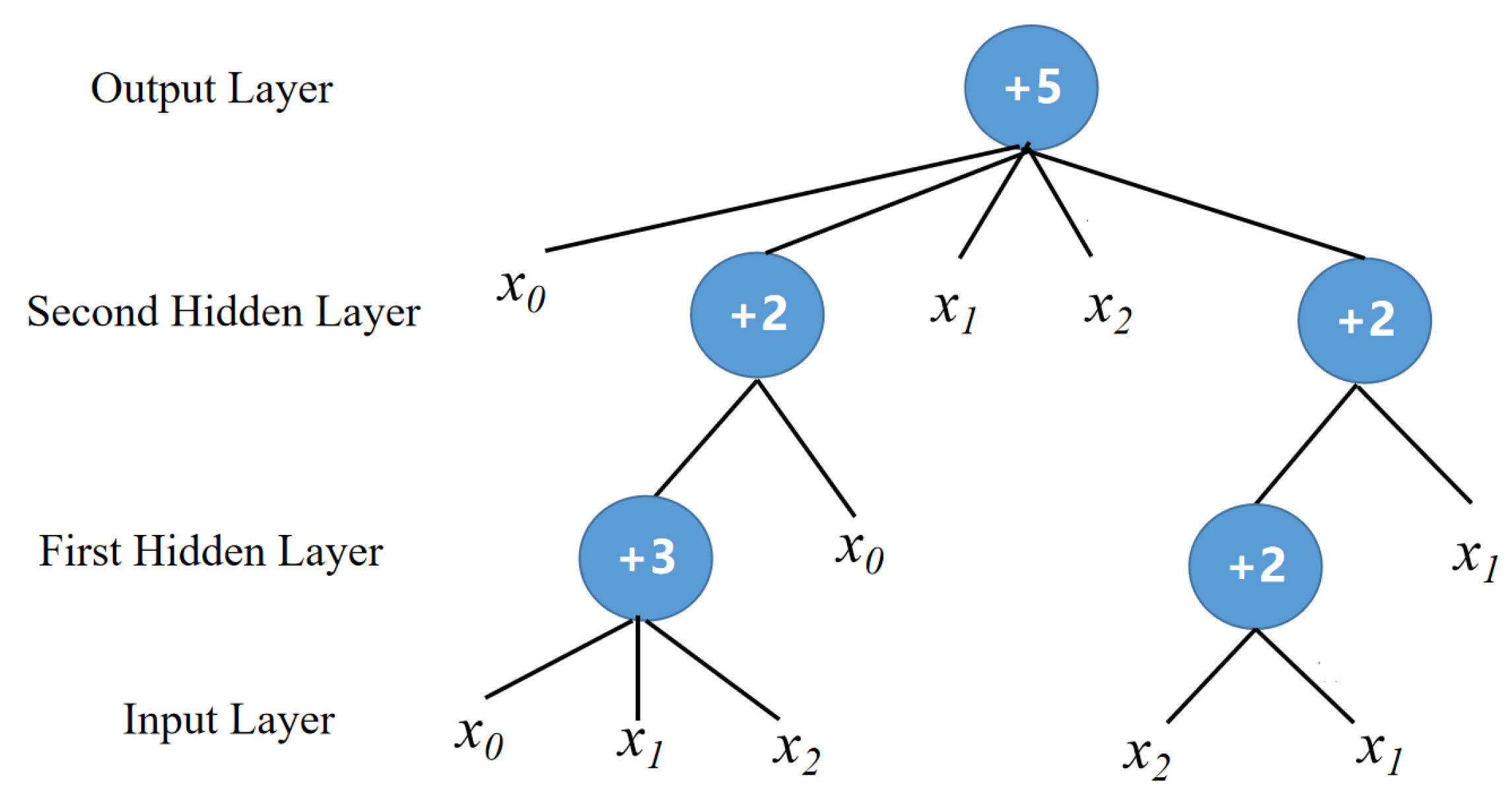
By employing genetic programming and particle swarm optimization algorithm (PSO), the structure and parameters of flexible neural tree (FNT) are designed to predict the traffic flow in the next-time frame, in which the variable inputs are allowed for covering many complicated factors in real-time traffic system concerning holidays and weather conditions;

(2)

A duration adjustment strategy of signal cycle is proposed for enhancing the intersection’s ability to undertake the overload or lightweight traffic flow in the next-time frame;

(3)

Linking the competitive relationship among the contradictory phases with the prediction traffic flow directly, an elastic adaption scheduling strategy for the separate phases’ green lights is derived from the analytical solution to achieve the adaptability for the upcoming traffic flow and make full use of the utilization of the presetting duration of signal cycle, which is obtained from a designed tradeoff scheduling optimization problem.

The structure of this paper is as follows: in Section 2, the framework for traffic light scheduling is proposed; Section 3 gives the algorithm for traffic flow prediction based on FNT model; the strategy of adaptation scheduling for urban traffic lights is designed in Section 4 in detail; the corresponding experiment results are given in Section 5; and this paper ends with a conclusion in Section 6.

2. Overall Frame Structure for Urban Traffic Light Scheduling

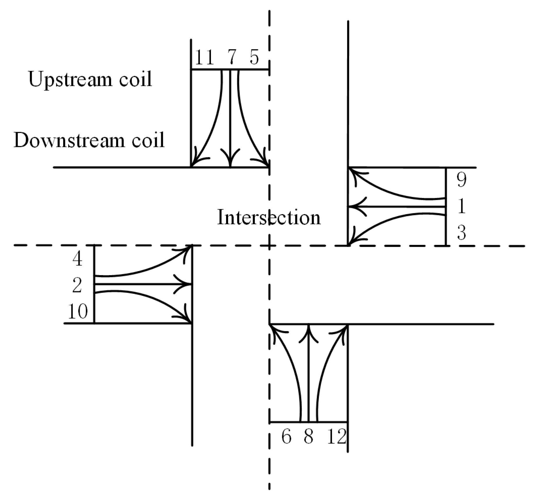
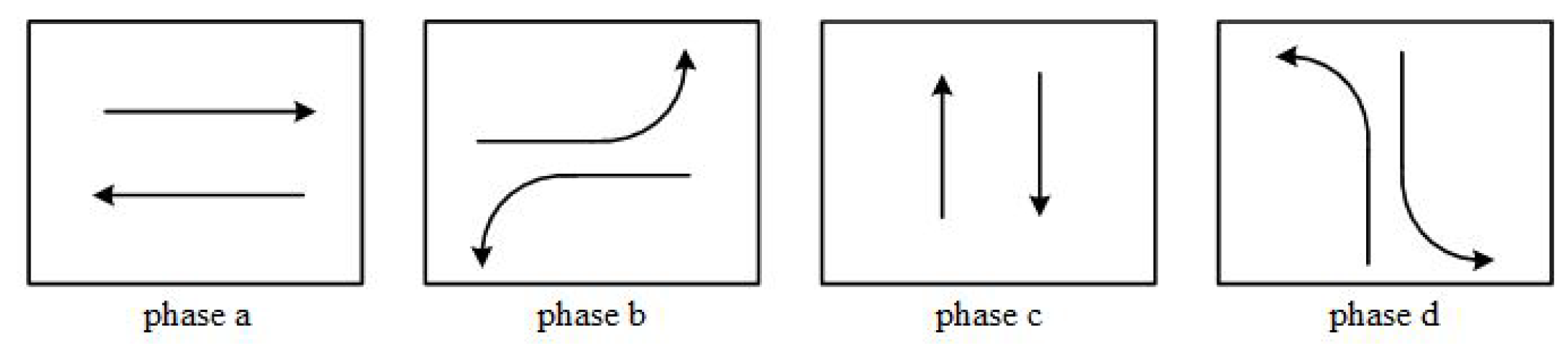
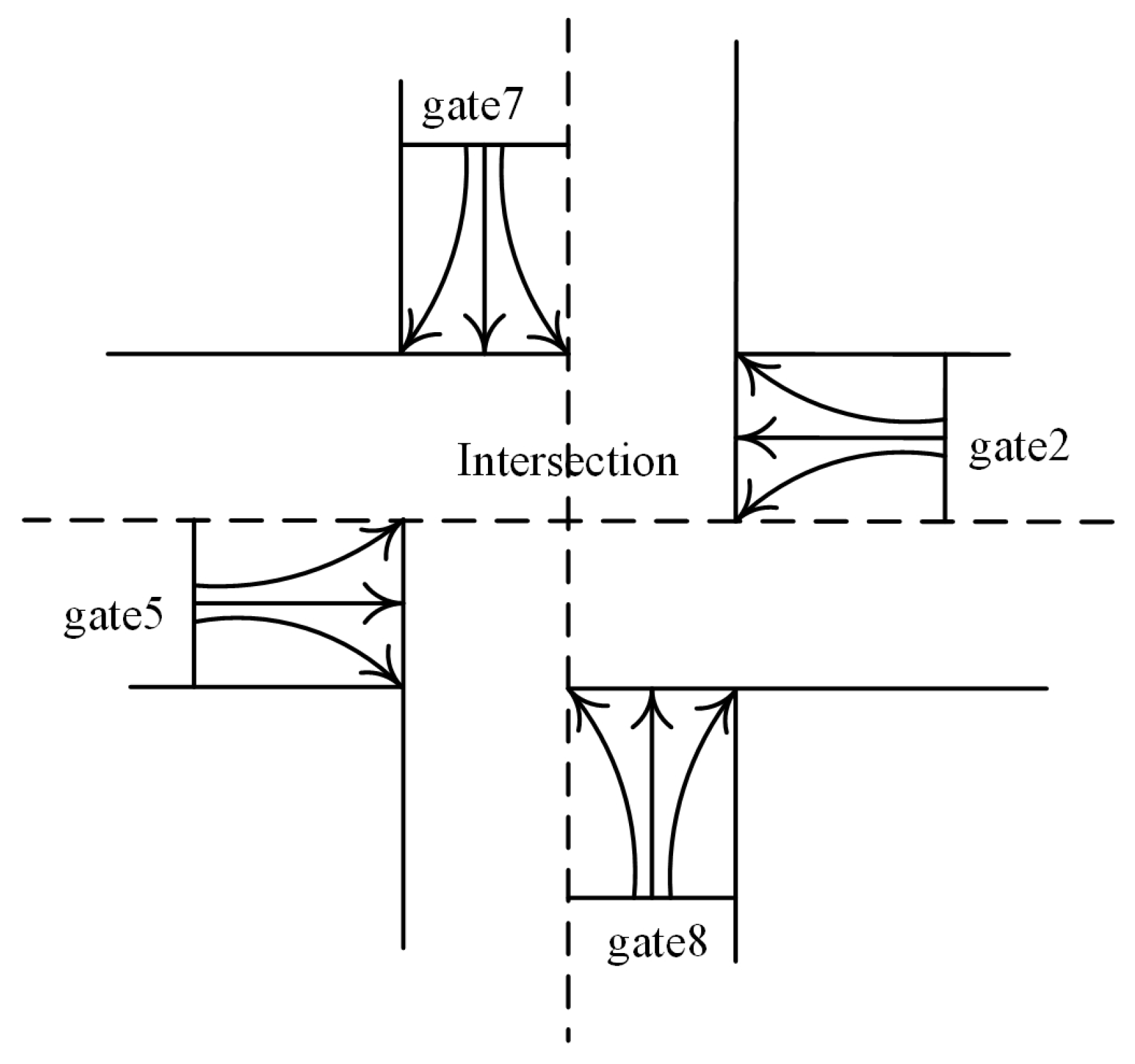
2.1. Signal Phases in Traffic Light Control Systems

In traffic light control systems, the signal phases are defined to avoid the conflict of traffic flow in different directions.

During a signal cycle in a traffic signal control system, a group of nonconflicting multidirectional traffic flows in the same signal phase go through the intersection under the preset order. Generally, the duration of signal cycle is divided into multiple time slices, which corresponds to the green-light signal for each signal phase. Thus, the scheduling objective of urban traffic light is the scheduling of time slices for the signal phases in the duration of a signal cycle. Meanwhile, the signal intersection could be classified based on the geometrical shape, including T shape, Y shape, X shape, ring cross shape and so on. Thus, a signal intersection can be viewed as an N-phase controlled intersection, where N represents the number of phases in an intersection.

For example, a typical intersection with four phases is displayed in Figure 1, in which the corresponding phases are shown in Figure 2. The preset order is $b\to a\to c\to d\to b$. Thus, a 4-phase controlled intersection can be formulated, in which the duration of a signal cycle is comprised of four time slices corresponding to the four phases of a green-light signal respectively.

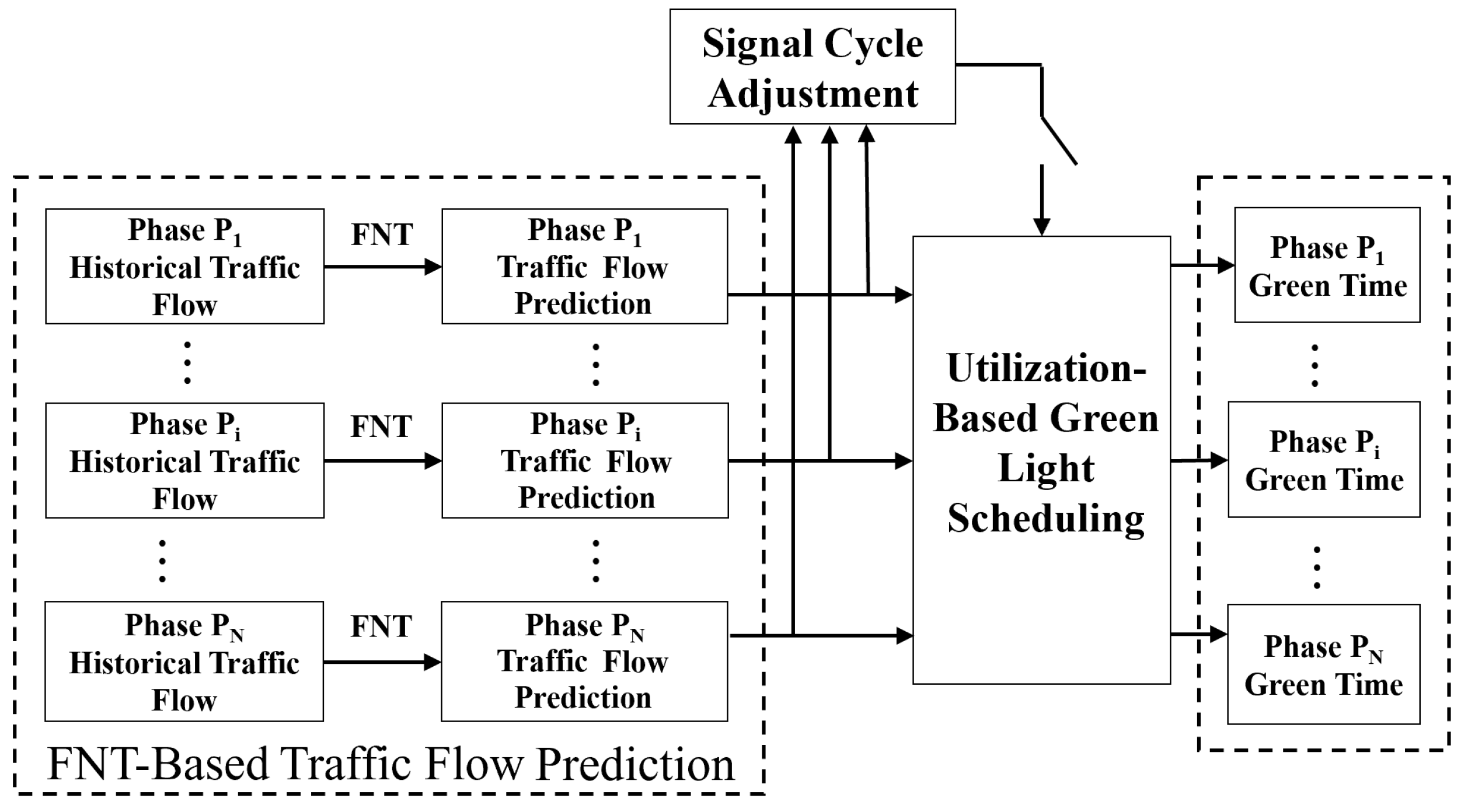
2.2. Framework for Traffic Light Adaptation Scheduling

The designed framework for traffic light scheduling is shown in Figure 3. It consists of three components: the FNT-based traffic flow prediction; the adjustment for the duration of the signal cycle; and the elastic utilization-based adaptive scheduling strategy for the intersection-phase green lights.

The first component of FNT-based traffic flow prediction provides the basic information for the other two components in the overall framework. In practice, the traffic light scheduling mainly depends on the upcoming traffic flow in each signal phase. In this component, a flexible neural tree model (FNT) is designed to predict the upcoming traffic flow $q_i\left(t\right)$ for the ith phase in an intersection in the next-time frame $T_f$. The previous traffic flow in each phase is collected to build the dataset. Here, many complicated factors are taken into consideration, such as weather and holidays.

Because the traffic flow changes over time in the next-time frame, an intersection may withstand the overload or lightweight traffic flow. While an overload or lightweight situation appears, the duration T of signal cycle could be adjusted before scheduling the green lights for each signal phase. Thus, an event-trigged strategy needs to be embedded into the adjustment component for the duration of signal cycle to enlarge or reduce the duration T. The duration T of signal cycle is the sum of the green-light duration of each phase, following that

$$T=\sum _{i=1}^N{T}_i,$$

(1)

where $T_i$ denotes the green-light duration of the ith phase in an intersection. At the beginning of the experiment, we assign an initial value of T and $T_i=T/N$. As the experiment progresses, the timing cycle will gradually approach the optimal timing cycle. Therefore, the second component is intended to adjust the duration of signal cycle based on the upcoming traffic flow.

Taking the most efficient utilization of the duration of signal cycle as the scheduling objectives, the component of elastic utilization-based adaptive scheduling strategy for signal-phase green lights is designed. Linking the prediction traffic flow of each phase directly to the green-light scheduling, a tradeoff scheduling optimization problem is formulated, in which the utilization U of the signal cycle depends on the sum of variance yields between the scheduling green time $T_i$ and the allowed maximum green light ${T_i}_{max}$, which is described as

$$U=\sum _{i=1}^N{({T_i}_{max}-T_i)}^2.$$

(2)

The smaller the value U under the necessary constrain condition, the better the utilization. Therefore, in this component, the adaptive scheduling strategy could provide the reasonable $T_i$ for each traffic phase to utilize the signal cycle effectively in the next-time frame.

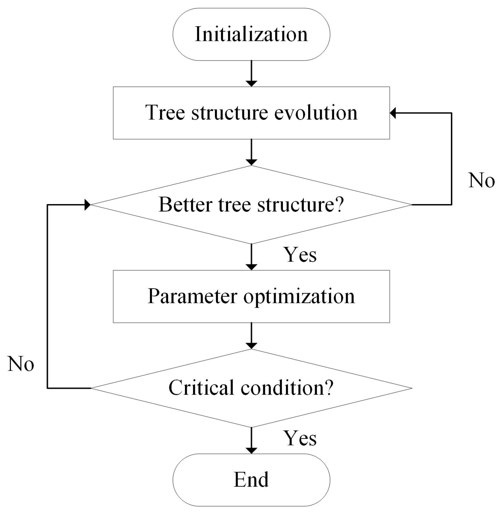
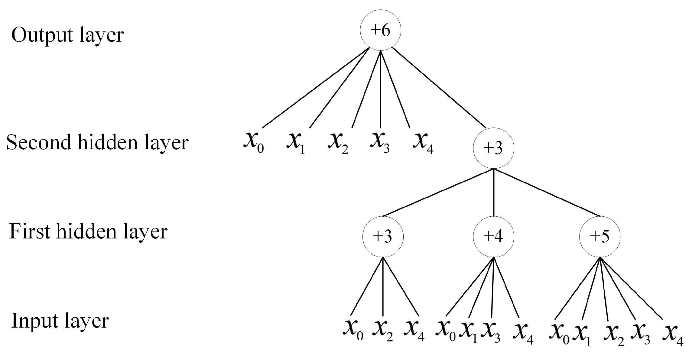
3. Signal Phase Traffic Flow Prediction via FNT

In this paper, the flexible neural tree is designed to predict the phase traffic flow in the next-time frame, which is an alternative tree structural neural network that solves the problem of structural design in the traditional neural networks [35,36]. A typical FNT model is displayed in Figure 4.

In order to generate the FNT structure and model, the function set F and terminal instruction set T are defined as

$$S=F\cup T=\{{+}_2,{+}_3,\dots ,{+}_N\}\cup \{x_1,\dots ,x_n\},$$

(3)

where $x_1,x_2,\dots ,x_n$ are the instructions of leaf nodes. The instructions ${+}_i(i=2,3,\dots ,N)$ are viewed as the flexible neuron operator. Once a nonterminal instruction is selected, the value i is randomly generated with two random adjustable parameters $a_i$ and $b_i$. Thus the output of ${+}_i$ is calculated by

$$Ou{t}_i=f(a_i,b_i,{\sum }_{i=1}^N{w}_j\times x_j)=e^{-{({\sum }_{i=1}^N{w}_j\times x_j-a_i/b_i)}^2},$$

(4)

where $x_j(j=1,2,3,\dots ,N)$ denote the inputs to node ${+}_i$ and $w_j(j=1,2,3,\dots ,N)$ denote the inertia weight to node ${+}_i$ obtained by PSO.

The process of generating a flexible neural tree consists of two main parts, namely the tree structure optimization and parameter optimization. This is shown in Figure 5. Grammar-guided genetic programming (GGGP) is employed to optimize the structure of the FNT, and particle swarm optimization (PSO) is introduced to optimize the relevant parameters. The pseudocode of PSO is shown in Algorithm 1.

In PSO algorithm, each particle represents a potential solution to the task within the search space. In the D-dimensional space, the position vector and velocity vector of the i-th particle can be expressed as $x_i=(x_{i1},x_{i2},\dots ,x_{iD})$ and $v_i=(v_{i1},v_{i2},\dots ,v_{iD})$, respectively. By using the random initialization of particles, the velocity and position of the ith particle are updated as follows

$$\begin{array}{c}{v}_i(t+1)=w{v}_i\left(t\right)+c_1{r}_1(p_i-x_i\left(t\right))+c_2{r}_2(p_g-x_i\left(t\right)),\hfill \\ x_i(t+1)=x_i\left(t\right)+v_i(t+1),\hfill \end{array}$$

(5)

where w is the inertia weight and can be used to control the influence of previous velocity on the new one; the parameters $c_1$ and $c_2$ are two constants which determine the weights of $p_i$ and $p_g$; $p_i$ represents the best previous position of the i-th individual and $p_g$ denotes the best previous position of all particles in current generation; $r_1$ and $r_2$ represent two separately generated random values which uniformly distribute in the range of $[0,1]$.

Algorithm 1: The particle swarm optimization (PSO)

1. Initialize popolation 2. for t = 1:maximun generation 3.    for i = 1:population size 4.       if $f\left(x_{i,d}\left(t\right)\right)<f\left(p_i\left(t\right)\right)$ then $(p_i\left(t\right)=x_{i,d}\left(t\right)$ 5.          $f(p_g\left(t\right)=min(f\left(p_i\left(t\right)\right)$ 6.       end 7.       for d = 1:dimension 8.          $v_i(t+1)=w{v}_i\left(t\right)+c_1{r}_1(p_i-x_i\left(t\right))+c_2{r}_2(p_g-x_i\left(t\right))$ 9.          $x_i(t+1)=x_i\left(t\right)+v_i(t+1)$ 10.          if $(v_{i,d}(t+1)>v_{max}$ then $(v_{i,d}(t+1)=v_{max}$ 11.          else if $(v_{i,d}(t+1)<v_{max}$ then $(v_{i,d}(t+1)=v_{min}$ 12.          end 13.          if $(x_{i,d}(t+1)>v_{max}$ then $(x_{i,d}(t+1)=x_{max}$ 14.          else if $(x_{i,d}(t+1)<v_{max}$ then $(x_{i,d}(t+1)=x_{min}$ 15.          end 16.       end 17.    end 18.  end

For predicting the upcoming traffic flow of signal phases, the dataset could be composed by the historical data of traffic flow for each signal phase, in which the traffic flow could be sliced based on the time frame $T_f$. After establishing the traffic flow dataset, the training data are normalized by using the following equation $x^{\prime }=(x-x_{min})/(x_{max}-x_{min})$. Meanwhile, datasets could be divided into $2/3$ as training set and $1/3$ for test set to obtain the structure of FNT for predicting the upcoming traffic flow for each phase. In order to obtain the near-optimal FNT, the following normalized mean squared error is designed as the fitness function, which is given by

$$Fi{t}_{FNT}=\frac{{\sum }_{k=1}^{N_{Tr}}{(x_k-{\widehat{x}}_k)}^2}{{\sum }_{k=1}^{N_{Tr}}{(x_k-\overline{x})}^2},$$

(6)

where $x_k$ and ${\widehat{x}}_k$ are the actual and output of FNT at kth sample; $\overline{x}$ represents the average value of traffic data; $Tr$ denotes the length of train samples.

Thus, based on FNT, the signal phase traffic flow prediction Algorithm 2 is described as follows.

Algorithm 2: Signal Phase Traffic Flow Prediction via FNT.

Require: The data set of historical traffic flow of each signal phase. 1. Normalize the traffic flow data: $x^{\prime }=(x-x_{min})/(x_{max}-x_{min})$; define the training set and test set; 2. Initialize the values of parameters used in GGGP and PSO; set the elitist program as $NULL$ and its fitness value as the biggest positive real number of the computer at hand. Then create the initial population; 3. Construct optimization using GGGP algorithm, in which the fitness function is calculated by root mean square error (RMSE); 4. If the better structure is found, then go to step 5, otherwise go back to step 3; 5. Optimize parameters using PSO algorithm; 6. If the maximum number of local search is reached, or no better parameter vector is found for a significantly long time, then go to step 7; otherwise go to step 5; 7. If the satisfied solution is found, then stop and save the prediction traffic flow $q_i$ of each signal phase; otherwise go to step 3; 8. Save and output $q_i$ as the prediction traffic flow of the ith phase.

The output $q_i$ of the trained FNT provides the decision-making information for the duration adjustment of signal cycle and the global utilization-based green-light adaption scheduling.

4. Adaptation Strategy for Urban Traffic Light Scheduling

4.1. Duration Adjustment for Signal Cycle Based on Traffic Flow Prediction

The duration depends not only on the upcoming traffic flow but also on the last duration of signal cycle. While obtaining the traffic flow prediction of each phases in an intersection, the evaluation q of the traffic load in the next-time frame could be calculated for the overall intersection, where $q={\sum }_{i=1}^N{q}_i$. Meanwhile, the evaluation q of traffic load and its one-step difference $\Delta q=q-q^{old}$ are employed to characterize the traffic load of overall intersection.

There are three scenarios for the traffic load q of overall intersection.

(1)

If the traffic load is too heavy (i.e., q is with large value) or is increased significantly (i.e., $\Delta q>0$ is with large positive number), the duration of signal cycle will be prolonged;

(2)

If the traffic load is too light (i.e., q is with small value) or is decreased significantly (i.e., $\Delta q<0$ is with large negative number), the duration of signal cycle will be reduced to save the intersection sources;

(3)

Otherwise, if the traffic load is neither heavy nor too light (i.e., q is with moderate value) or is changed smoothly (i.e., $\Delta q$ is with moderate value), the duration of signal cycle will be maintained and the green time for each phase will be scheduled directly in the next-time frame.

In order to cover the above scenarios of traffic load in overall intersection and guide the duration adjustment for signal cycle, the following traffic flow index is introduced to describe the variation trend in the next-time frame of traffic load, which is described as

$$TP=\alpha q+(1-\alpha )\Delta q,\alpha \in [0,1],$$

(7)

where $\alpha$ is the memory weight factor of traffic flow.

Based on the designed traffic load characterization in (6), the following three strategies are proposed for adjusting the duration of signal cycle in the next-time frame.

(1)

When $TP$ is bigger than a maximum threshold $T{P}^H$, the traffic flow is too heavy. Thus set T to its maximum $T_{max}$ according to

$$T^{new}=T_{max},with{T}_{max}={\sum }_{i=1}^N{T_i}_{max},$$

(8)

where ${T_i}_{max}$ is the allowed maximum green time of the ith phase in an intersection.

(2)

When $TP$ is smaller than a minimum threshold $T{P}^L$, the traffic flow is too light. Thus, set T to its minimum $T_{min}$ according to

$$T^{new}=T_{min},with{T}_{min}={\sum }_{i=1}^N{T_i}_{min},$$

(9)

where ${T_i}_{min}$ is the allowed minimum green time of the ith phase in an intersection.

(3)

Otherwise, i.e., $TP$ is between $T{P}^L$ and $T{P}^H$, set T between its upper and lower bounds according to

$$\begin{array}{c}{T}^{new}=T_{max}-\frac{T_{max}-T_{min}}{T{P}^H-T{P}^L}(TP-T{P}^L),ifT{P}^L<TP<T{P}^H.\hfill \end{array}$$

(10)

Based on the above strategies, the new duration $T^{new}$ of signal cycle in the next-time frame can be obtained.

4.2. Elastic Utilization-Based Adaptive Scheduling for Phase Green Light

As stated in the architecture of the overall framework, while setting the duration of signal cycle in the next-time frame, the green-light duration $T_i$ of each phase could be scheduled to make full use of the utilization of the presetting duration of signal cycle $T^{new}$.

Linking the utilization of duration of signal cycle with the prediction traffic flow of signal phases, the following quadratic programming problem is formulated first, which is given by

$$\begin{array}{c}min:E(T_1,T_2,\dots ,T_N)={\displaystyle \sum _{i=1}^N}{w}_i\left(t\right){(T_{i_{max}}-T_i)}^2,\hfill \\ s.t.:{\displaystyle \sum _{i=1}^N}{T}_{i_{max}}\ge T,{\displaystyle \sum _{i=1}^N}{T}_i=T,T_i\ge T_{i_{min}},T_i<T_{i_{max}},\hfill \\ i=1,2,\dots ,N,\hfill \end{array}$$

(11)

where $w_i\left(t\right)=q_i/{q_i}_{max}$ denotes relative traffic load of the ith phase in the next-time frame, in which ${q_i}_{max}$ represents the allowed maximum traffic flow of the ith phase in a time frame.

Remark 1.

In order to minimize the value of $E(T_1,T_2,\dots ,T_N)$ in (10), the allocated traffic green light $T_i$ is closer to ${T_i}_{max}$ with the corresponding relatively heavier traffic load $w_i\left(t\right)$.

Under the constrained conditions in (11), by using the Karush–Kuhn–Tucker (KKT) condition and the Lagrange multiplier method, the optimal analytical solution ${T_i}^{new}$ is produced while $\widehat{T}>T$ and $T_i>T_{i_{max}}$, where $\widehat{T}={\sum }_{T_i\ne T_{i_{max}}}{T}_{i_{max}}+{\sum }_{T_i\ne T_{i_{max}}}{T}_{i_{min}}$, and can be described as

$${T_i}^{new}=T_{i_{max}}-\frac{\frac{1}{w_i}(\widehat{T}-T)}{{\sum }_{T_j\ne T_{j_{min}}}(1/w_j)};$$

(12)

otherwise, ${T_i}^{new}=T_{i_{min}}$.

Thus the scheduling durations of green lights for signal phases are the analytical solution $T_1,T_2,\dots ,T_N$ obtained from (12).

4.3. Algorithm for Adaptation Scheduling for Urban Traffic Light

Following the output $q_i$ of FNT in Section 3, by integrating the duration adjustment for the signal cycle in (8)–(10), and the proposed elastic utilization-based adaptive scheduling for phase green light in (12), the Algorithm 3 for the adaptation scheduling of urban traffic lights is described as follows.

Algorithm 3: Adaptation Scheduling of Urban Traffic Lights.

Require: The set of signal phases, $P_1,P_2,\dots ,P_N$; the data set of historical traffic flow of each signal phase; the preset order of signal phases; the trained structure of FNT for prediction traffic flow for each phases. Obtain the prediction traffic flow $q_i$ of each phase via FNT; obtain the traffic flow index $TP$; Set the initial parameters of T, q, $\alpha$, $T_{max}$, $T_{min}$, $T{P}^L$, and $T{P}^H$; Set the constant of signal phases, $\overline{T}$, ${q_i}_{max}$, ${T_i}_{max}$ and ${T_i}_{min}$; Calculate the duration T of signal cycle: if$TP>T{P}^H$ then $T^{new}:=T_{max}$; else if$TP<T{P}^L$ then $T^{new}:=T_{min}$; else$T^{new}:=T_{max}-\frac{T_{max}-T_{min}}{T{P}^H-T{P}^L}(TP-T{P}^L)$; end if Update $T=T^{new}$, $w_i\left(t\right)=q_i/{q_i}_{max}$; Calculate the green light $T_i$ of signal phase: if$\widehat{T}>T$ and $T_i>T_{i_{max}}$ then ${T_i}^{new}=T_{i_{max}}-\frac{\frac{1}{w_i}(\widehat{T}-T)}{{\sum }_{T_j\ne T_{j_{min}}}(1/w_j)}$; else${T_i}^{new}=T_{i_{min}}$; end if Save and output the result $T_i={T_i}^{new}$.

5. Simulation Results and Analysis

An intersection, named Dongying Economic Development Zone located in Shandong Province in China, is employed to verify the effectiveness of the proposed algorithm for the adaptation scheduling of urban traffic lights, including four directions, four phases, and three lanes. Let us take one of the roads: the lanes in one direction are divided from left to right into one left-turning lane, one straight-going lane and one right-turning lane. The lanes are 3.5 m wide. Each vehicle follows a fixed route, which is engendered at random. The corresponding relationship between the four directions of intersection and each gate is shown in Figure 6.

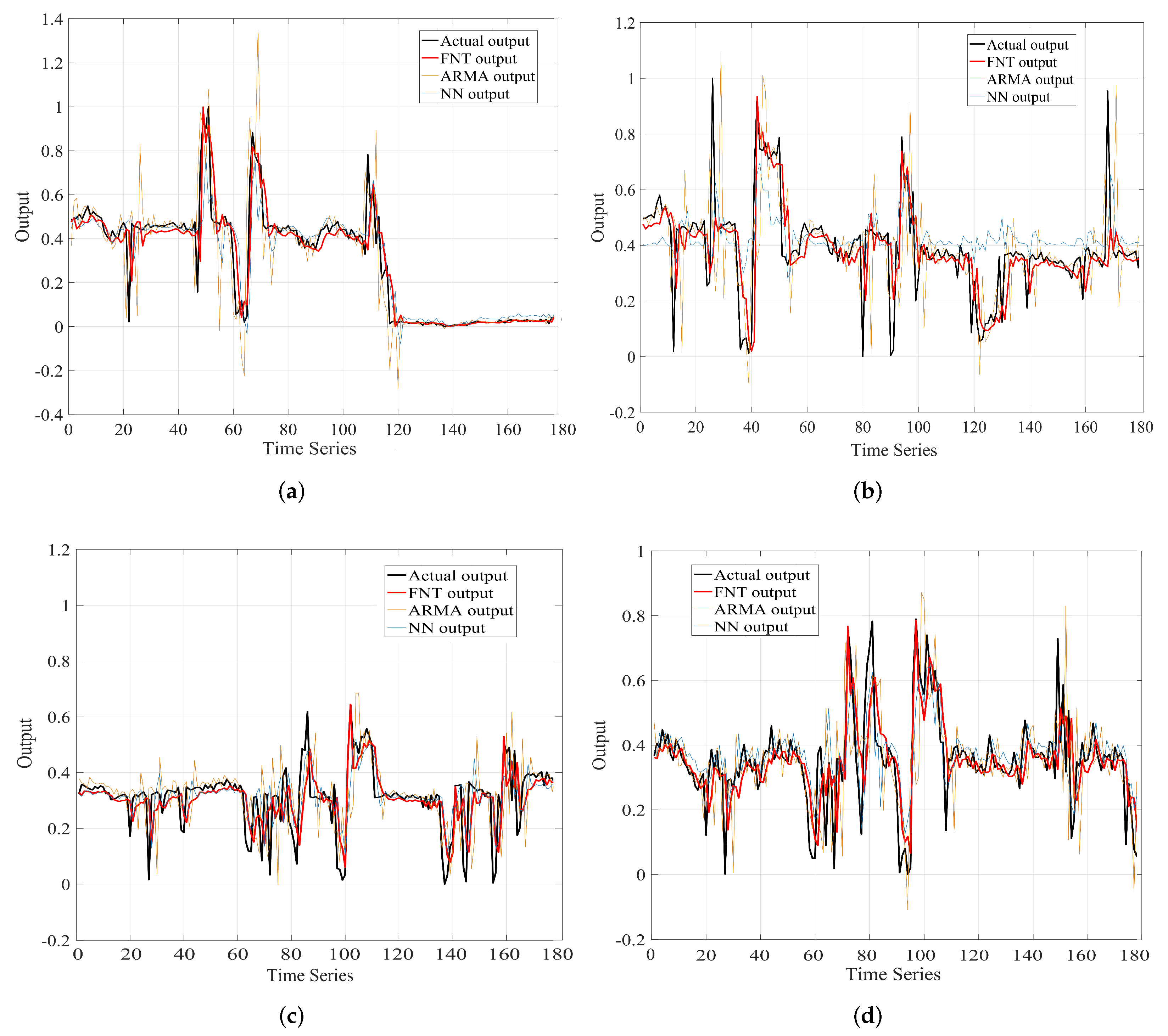
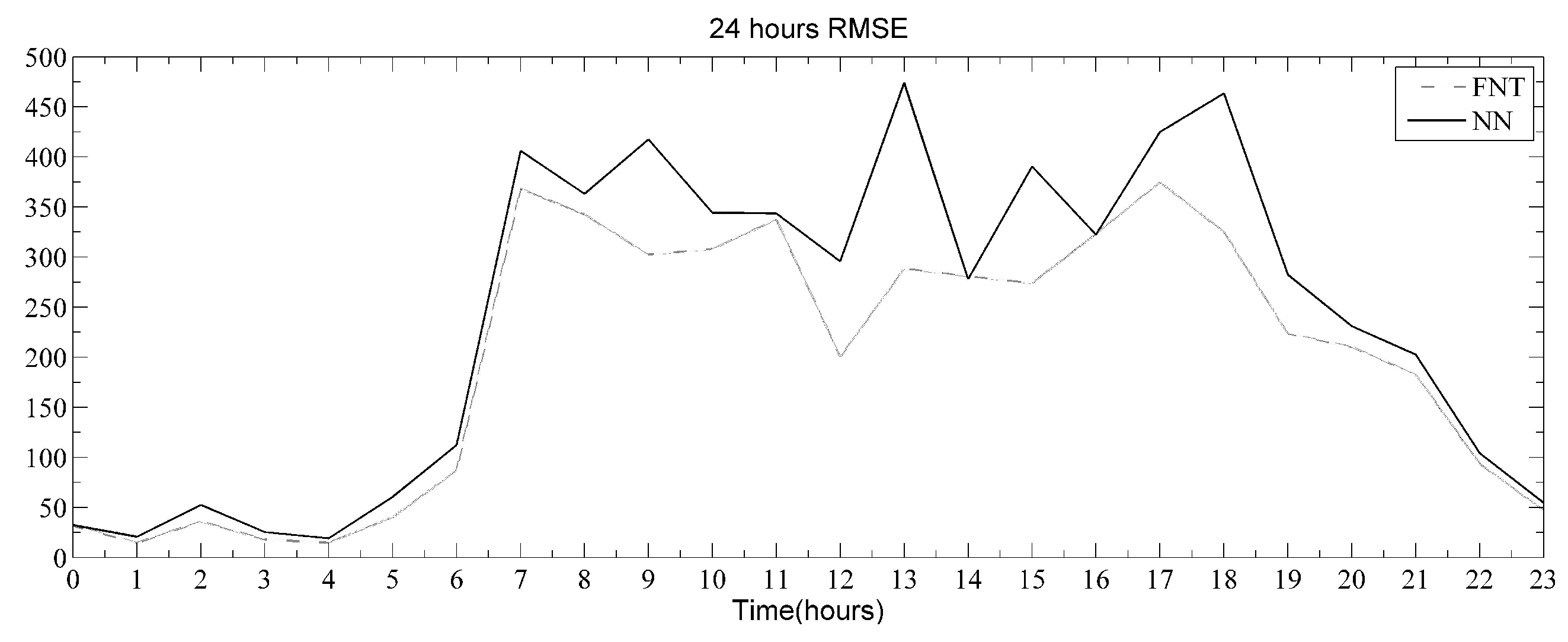
5.1. Performance of Traffic Flow Prediction via FNT

In this subsection, the performance of the designed traffic flow prediction algorithm is illustrated.

More specially, the data package contains 1 h’s worth of traffic flow from Monday to Friday. The length of this traffic data package is 18,000. Setting the prediction time interval $T_f$ as 1 h, the objective of FNT is to predict the traffic flow every hour on Monday. The function set F and terminal instruction set T of FNT are defined as $S=F\cup T=\{{+}_2,{+}_3,\dots ,{+}_6\}\cup \{x_0,x_1,\dots ,x_4\}$. The trained structure of flexible neural tree is shown in Figure 7.

After that, the comparison results under different prediction algorithms are displayed to prove the effectiveness of FNT, including autoregressive moving average method (ARMA), neural network (NN), and FNT. Furthermore, the prediction results of traffic flow on four gates at 8 o’clock, obtained from the ARMA, NN, and FNT, are shown in Figure 8, where the x-axis and y-axis represent the number of time series and the normalized prediction number of traffic flow, respectively. Figure 9 shows the 24 h RMSE values in gate 2 under FNT and NN, in which the x-axis represents the 24 h in a day, and y-axis represents the RMSE value for 1 hour. Meanwhile, the comparison results between real traffic flow data and forecast data of gate 2 are shown in

Table 1. The true and forecast traffic data in gate 2.

	Traffic Flow	(Vehicle)		Traffic Flow	(Vehicle)		Traffic Flow	(Vehicle)
Time (Hour)	True Data	Forescast Data	Time (Hour)	True Data	Forescast Data	Time (Hour)	True Data	Forescast Data
0	22	29	8	452	342	16	422	352
1	15	13	9	387	317	17	482	328
2	10	11	10	333	315	18	577	446
3	15	11	11	397	351	19	376	305
4	17	16	12	227	164	20	207	172
5	28	34	13	277	189	21	165	141
6	102	88	14	425	353	22	109	80
7	454	178	15	394	387	23	41	36

.

Observed from Figure 5, the prediction of variation tendency in three curves under ARMA, FNT, and NN are almost the same. However, compared to ARMA, the curves under the FNT model are closer to the actual traffic flow. It demonstrates that due to the complexity of the real traffic flow, linear models such as ARMA cannot predict as expected. Meanwhile, it could be found from Table 1 that the difference between the predicted data and the true traffic data under FNT is smaller than those under NN. Based on the above simulation results, the FNT-based algorithm for predicting traffic flow could provide the accurate traffic data for scheduling the traffic lights.

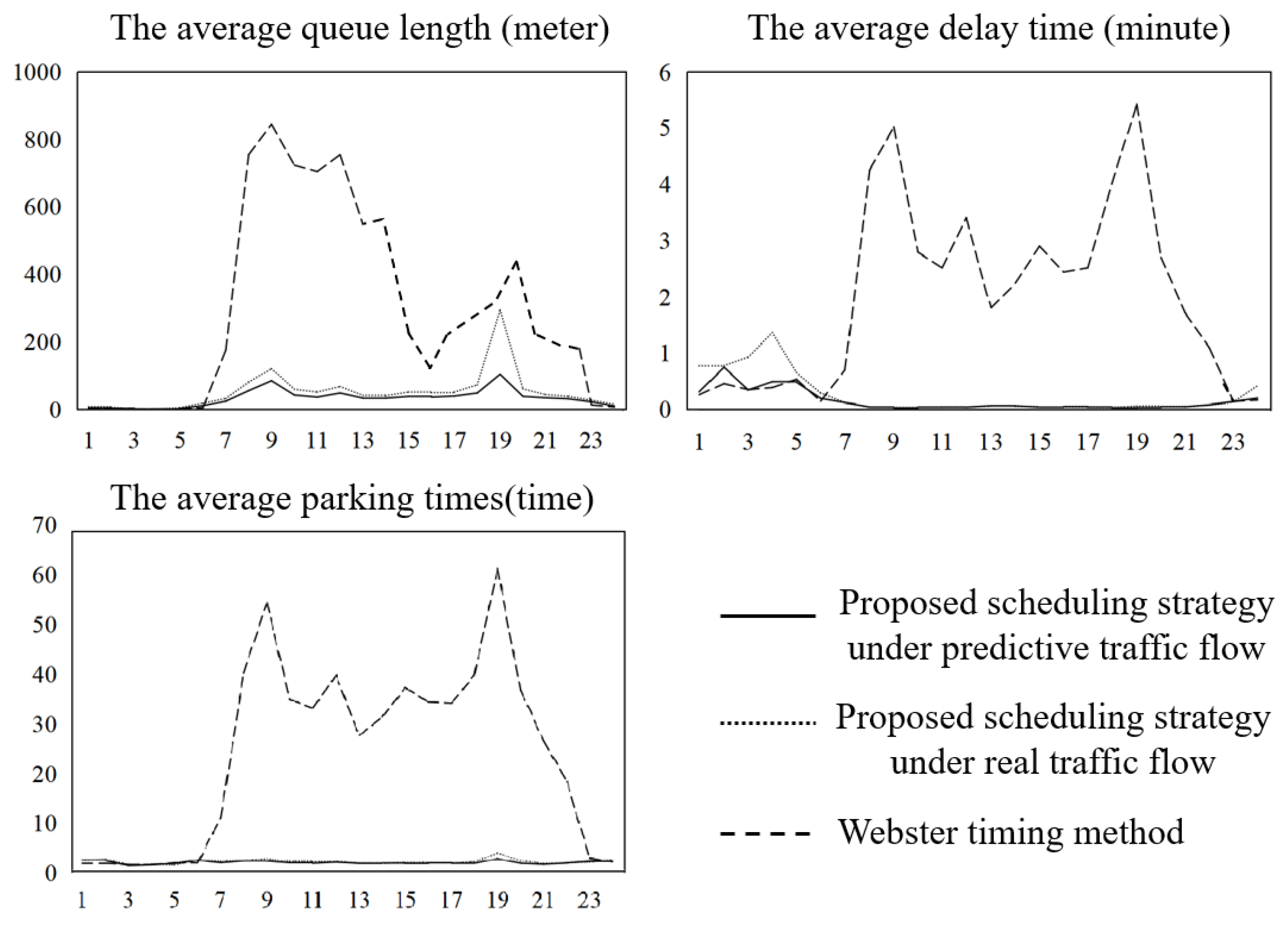
5.2. Performance of Adaptation Scheduling Algorithm of Urban Traffic Light

By simulating the traffic condition in Dongying Economic Development Zone under the proposed adaptation scheduling algorithm, simulation results are given and discussed in this subsection.

Three performance indices are selected to evaluate the scheduling traffic light methods, including the average queue length, the average delay time, and the average parking time. Based on the prediction results of traffic flow on a certain day obtained from Section 5.1, the comparison results under different traffic light methods are shown in Figure 10, including Webster timing method, the proposed scheduling algorithm under real and predictive traffic flow, where x-axes represent 24 h in 1 day.

Generally speaking, the shorter the length of the average queue, the shorter the time duration of the average delay, and the fewer the parking times, the better the scheduling strategy. From the comparison results in Figure 9, it could be seen clearly that the variation tendency of the proposed scheduling algorithm under real and predictive traffic flow were approximately the same. The Webster timing method is the worst. While the traffic flow is relatively large, the performance indices become poor. Even under a heavy traffic flow at 8 o’clock, the proposed scheduling strategy still shows good performance. Meanwhile, the proposed scheduling strategy has obvious advantages in the two performance indicators of average queue length and average parking times, especially at 18 o’clock. Meanwhile, the difference between the proposed scheduling algorithm under real and predictive traffic flow is mainly caused by the prediction error.

In summary, the proposed scheduling strategy performs better for matching the prediction of the traffic flow with the timing of the traffic light. Thus the average queue length, the average delay time and the average parking time with lower values could be obtained.

6. Conclusions and Future Work

In this paper, a strategy for traffic light scheduling has been proposed to enhance the flexibility of adaptation to traffic fluctuation. The FNT model was designed to predict the traffic flow of each phase at an intersection. A duration adjustment strategy of signal cycle has been designed to deal with the traffic scenarios of overload or lightweight traffic flow in the next-time frame. After that, an elastic adaption scheduling strategy of separate phases’ green lights has been proposed based on a designed tradeoff scheduling optimization problem. The fast-moving traffic at a single intersection may put extra pressure on other adjoining intersections. So, the next experiment will cover multiple intersections to achieve a fast traffic flow in the road network.

Due to the development of artificial intelligence technologies, in the future, it will be worthwhile to embed other intelligent methods into the framework proposed in this work to improve the performance of traffic light scheduling, such as combining the advanced graph neural network and mathematical model into the component of traffic flow prediction, integrating the reinforced learning into the component of traffic light scheduling, and so on.

References

1. Chen, L.-W.; Hu, T.-Y. Flow equilibrium under dynamic traffic assignment and signal controlan illustration of pretimed and actuated signal control policies. IEEE Trans. Intell. Transp. Syst. 2012, 13, 1266–1276. [Google Scholar] [CrossRef]
2. Pacheco, A.; Simoes, M.L.; Milheiro-Oliveira, P. Queues with server vacations as a model for pretimed signalized urban traffic. Transp. Sci. 2017, 51, 841–851. [Google Scholar] [CrossRef] [Green Version]
3. Spall, J.C.; Chin, D.C. Traffic-responsive signal timing for system-wide traffic control. Transp. Res. Part C Emerg. Technol. 1997, 5, 153–163. [Google Scholar] [CrossRef]
4. Li, Y.-Q.; Li, K.; Feng, Y.-J. Data-driven traffic-responsive green wave coordinated signal control. Control Theory Appl. 2016, 33, 588–598. [Google Scholar]
5. Jin, J.; Ma, X.; Kosonen, I. An intelligent control system for traffic lights with simulation-based evaluation. Control Eng. Pract. 2017, 58, 24–33. [Google Scholar] [CrossRef] [Green Version]
6. Zhao, D.; Dai, Y.; Zhang, Z. Computational intelligence in urban traffic signal control: A survey. IEEE Trans. Syst. Man Cybern. Part C Appl. Rev. 2012, 42, 485–494. [Google Scholar] [CrossRef]
7. Liang, X.; Du, X.; Wang, G.; Han, Z. A deep reinforcement learning network for traffic light cycle control. IEEE Trans. Veh. Technol. 2019, 68, 1243–1253. [Google Scholar] [CrossRef] [Green Version]
8. Vilarinho, C.; Tavares, J.P.; Rossetti, R.J.F. Design of a multiagent system for real-time traffic control. IEEE Intell. Syst. 2016, 31, 68–80. [Google Scholar] [CrossRef]
9. Shirvani, S.M.J.; Maleki, H.R. Maximum green time settings for traffic-actuated signal control at isolated intersections using fuzzy logic. Int. J. Fuzzy Syst. 2017, 19, 247–256. [Google Scholar] [CrossRef]
10. Wang, Y.; Zhou, J.; Wang, R.; Chen, L.; Chen, C.L.P.; Zhang, T.; Han, S. Transfer Collaborative Fuzzy Clustering in Distributed Peer-to-Peer Networks. IEEE Trans. Fuzzy Syst. 2022, 30, 500–514. [Google Scholar]
11. Grandinetti, P.; Canudas-de-Wit, C.; Garin, F. Distributed optimal traffic lights design for large-scale urban networks. IEEE Trans. Control Syst. Technol. 2019, 27, 950–963. [Google Scholar] [CrossRef] [Green Version]
12. Han, S.Y.; Zhou, J.; Chen, Y.H. Active fault-tolerant control for discrete vehicle active suspension via reduced-order observer. IEEE Trans. Syst. Man Cybern. Syst. 2021, 51, 6701–6711. [Google Scholar] [CrossRef]
13. Knorn, S.; Teixeira, A. Effects of jamming attacks on a control system with energy harvesting. IEEE Control Syst. Lett. 2019, 3, 29–34. [Google Scholar] [CrossRef]
14. Li, L.; Qin, L.; Xu, X.; Zhang, J.; Wang, Y.; Ran, B. Day-ahead traffic flow forecasting based on a deep belief network optimized by the multi-objective particle swarm algorithm. Knowl.-Based Syst. 2019, 172, 1–14. [Google Scholar] [CrossRef]
15. Tian, Y.; Zhang, K.; Li, J.; Lin, X.; Yang, B. LSTM-based traffic flow prediction with missing data. Neurocomputing 2018, 318, 297–305. [Google Scholar] [CrossRef]
16. Wu, Y.; Tan, H.; Qin, L.; Ran, B.; Jiang, Z. A hybrid deep learning based traffic flow prediction method and its understanding. Transp. Res. Part C Emerg. Technol. 2018, 90, 166–180. [Google Scholar] [CrossRef]
17. Habtemichael, F.G.; Cetin, M. Short-term traffic flow rate forecasting based on identifying similar traffic patterns. Transp. Res. Part C Emerg. Technol. 2016, 66, 61–78. [Google Scholar] [CrossRef]
18. Zhang, K.; He, F.; Zhang, Z.; Lin, X.; Li, M. Graph attention temporal convolutional network for traffic speed forecasting on road networks. Transp. B Transp. Dyn. 2021, 9, 622–640. [Google Scholar] [CrossRef]
19. Yu, J.Q.; Markos, C.; Zhang, S. Long-term urban traffic speed prediction with deep learning on graphs. IEEE Trans. Intell. Transp. Syst. 2021. [Google Scholar] [CrossRef]
20. Guo, K.; Hu, Y.; Sun, Y.; Qian, S.; Gao, J.; Yin, B. Hierarchical Graph Convolution Networks for Traffic Forecasting. Proc. AAAI Conf. Artif. Intell. 2021, 35, 151–159. [Google Scholar]
21. Guo, K.; Hu, Y.; Qiang, Z.S.; Liu, H.; Zhang, K.; Sun, Y.; Guo, J.; Yin, B. Optimized graph convolution recurrent neural network for traffic rrediction. IEEE Trans. Intell. Transp. Syst. 2021, 22, 1138–1149. [Google Scholar] [CrossRef]
22. Wu, Z.; Pan, S.; Long, G.; Jiang, J.; Zhang, C. Graph waveNet for deep spatial-temporal graph modelling. arXiv 2019, arXiv:1906.00121. [Google Scholar]
23. Carlos, Z.-G.; Chris, H. Expert system for traffic signal setting assistance. J. Transp. Eng. 1987, 113, 108–126. [Google Scholar]
24. Porto, W., Jr.; Ferreira, A.C.M. Suggestions for a new traffic signal setting. Inf. Tecnol. 1997, 8, 305–315. [Google Scholar]
25. Zhu, L.; Yu, F.R.; Wang, Y.; Ning, B.; Tang, T. Big data analytics in intelligent transportation systems: A survey. IEEE Trans. Intell. Transp. Syst. 2019, 20, 383–398. [Google Scholar] [CrossRef]
26. Wolshon, A.B. Analysis of intersection delay under real-time adaptive signal control. Transp. Res. Part C Emerg. Technol. 1999, 7, 53–72. [Google Scholar] [CrossRef]
27. Robertson, D.I.; Bretherton, R.D. Optimizing networks of traffic signals in real time-the scoot method. IEEE Trans. Veh. Technol. 1991, 40, 11–15. [Google Scholar] [CrossRef]
28. Aoyama, K. Universal Traffic Management System (UTMS) in Japan. In Proceedings of the VNIS’94—1994 Vehicle Navigation and Information Systems Conference, Yokohama, Japan, 31 August–2 September 1994; pp. 619–622. [Google Scholar]
29. Jayakrishnan, R.; Mahmassani, H.S. An evaluation tool for advanced traffic information and management systems in urban networks. Transp. Res. Part C Emerg. Technol. 1994, 2, 129–147. [Google Scholar] [CrossRef]
30. Ossama, Y.; Nader, M. Employing cyber-physical systems: Dynamic traffic light control at road intersections. IEEE Internet Things J. 2017, 4, 2286–2296. [Google Scholar]
31. Na, W.; Lee, Y.; Dao, N.N.; Vu, D.N.; Masood, A.; Cho, S. Directional link scheduling for real-time data processing in smart manufacturing system. IEEE Internet Things J. 2018, 5, 3661–3671. [Google Scholar] [CrossRef]
32. Tian, Y.; Jiang, X.; Levy, D.; Agrawala, A. Local adjustment and global adaptation of control periods for QoC management of control systems. IEEE Trans. Control Syst. Technol. 2012, 20, 846–854. [Google Scholar] [CrossRef] [Green Version]
33. Tian, Y.; Li, G. QoC Elastic scheduling for real-time control systems. Real-Time Syst. 2011, 47, 534–561. [Google Scholar] [CrossRef] [Green Version]
34. Liang, X.; Guler, S.I.; Gayah, V.V. An equitable traffic signal control scheme at isolated signalized intersections using Connected Vehicle technology. Transp. Res. Part C Emerg. Technol. 2020, 110, 81–97. [Google Scholar] [CrossRef]
35. Chen, Y.; Yang, B.; Dong, J.; Abraham, A. Time-series forecasting using flexible neural tree model. Inf. Sci. 2005, 174, 219–235. [Google Scholar] [CrossRef]
36. Yang, B.; Chen, Y.H.; Jiang, M.Y. Reverse engineering of gene regulatory networks using flexible neural tree models. Neurocomputing 2013, 99, 458–466. [Google Scholar] [CrossRef]
Figure 1. The geometric description of a four-phase intersection.
Electronics 11 00658 g001
Figure 2. Phases in an intersection.
Electronics 11 00658 g002
Figure 3. Framework for traffic light scheduling.
Electronics 11 00658 g003
Figure 4. The algorithm flowchart of FNT.
Electronics 11 00658 g004
Figure 5. The algorithm flow chart of FNT.
Electronics 11 00658 g005
Figure 6. The corresponding relationship between the four directions of intersection and each gate.
Electronics 11 00658 g006
Figure 7. The trained structure of FNT.
Electronics 11 00658 g007
Figure 8. Comparison results of the traffic flow prediction under ARMA, NN, and FNT at 8 o’clock. (a) The comparison results of traffic flow prediction on gate 2. (b) The comparison results of traffic flow prediction on gate 5. (c) The comparison results of traffic flow prediction on gate 7. (d) The comparison results of traffic flow prediction on gate 8.
Electronics 11 00658 g008
Figure 9. The 24 h RMSE values under FNT and NN in gate 2.
Electronics 11 00658 g009
Figure 10. Comparison average values of the queue length, delay time, and parking times.
Electronics 11 00658 g010