Abstract
Predicting stock market prices is an important and interesting task in academic and financial research. The volatile nature of the stock market means that predicting stock market prices is a challenging task. However, recent advancements in machine learning, especially in deep learning techniques, have made it possible for researchers to use such techniques to predict future stock trends based on historical financial data, social media news, financial news, and stock technical indicators (STIs). This work focused on the prediction of closing stock prices based on using ten years of Yahoo Finance data of ten renowned stocks and STIs by using 1D DenseNet and an autoencoder. The calculated STIs were first used as the input for the autoencoder for dimensionality reduction, resulting in less correlation between the STIs. These STIs, along with the Yahoo finance data, were then fed into the 1D DenseNet. The resultant features obtained from the 1D DenseNet were then used as input for the softmax layer residing inside the 1D DenseNet framework for the prediction of closing stock prices for short-, medium-, and long-term perspectives. Based on the predicted trends of the stock prices, our model presented the user with one of three suggested signals, i.e., buy, sell, or hold. The experimental results showed that the proposed approach outperformed the state-of-the-art techniques by obtaining a minimum MAPE value of 0.41.
1. Introduction
Predicting stock market prices has always been challenging [1,2] because of their long-term instability. The old market theory considers it difficult to forecast stock prices and that stocks perform at random. However, current scientific investigations indicate that high stock standards are reflected in earlier archives. Therefore, knowledge of the change developments is required to forecast values efficiently [3]. Furthermore, stock market companies and movements are influenced by numerous financial aspects, such as governmental proceedings, common commercial circumstances, product value indicators, stockholders’ anticipations, development of more stock markets, and the consciousness of shareholders [4]. The cost of stock units is calculated through high-level market capitalization. Various scientific factors allow numerical facts regarding the stock values [5]. Usually, stock indicators are increased from rates of stocks, along with high-level market assets, and they frequently evaluate the financial status in every nation. For instance, discoveries demonstrated that financial development in countries is certainly squeezed by stock market capitalization [6]. The description of a stock price change is vague and becomes risky for shareholders. Additionally, it is generally hard to identify the market significance for the administration. The stock principles are mostly vibrant, nonlinear, and non-parametric; hence, they regularly lead to the low performance of the mathematical models and incapacity to forecast the correct principles and developments [7].
Generally, traditional time-series forecasting techniques are based on static developments; thus, estimating stock values is the fundamental problem [8]. Additionally, predicting the stock trend is a major problem due to the included variables. Therefore, the market performs like a voting machine in the short term [9]. However, in the longer term, it acts as a weighing machine and, hence, there is scope for predicting the market movements for a more extended timeframe [10]. Machine learning (ML) is the most effective technique; it comprises various methods to improve a specific case study’s performance efficiently. According to previous research, ML can identify different patterns and effective information from the dataset [11]. Compared to traditional ML methods, the ensemble techniques are ML-based, where several ordinary procedures are employed to solve a specific challenge and were shown to outperform each of the approaches while calculating a time series [12,13]. For prediction challenges, boosting and bagging are efficient and prevalent techniques and ensemble methods.
The advancement of deep-learning-based methods in several fields, e.g., text analysis, trends prediction, and image analysis, have urged researchers to explore them in the field of stocks as well. Therefore, numerous DL-based approaches have been presented to predict the future trends of stocks. DL is the extended form of multilayer ANN-based ML approaches, which are empowered enough to enhance the prediction accuracy of algorithms. Due to the extensive advantages and power of DL techniques, these methods have shown better performance in stock price prediction.
Even though several studies [14,15,16] were presented regarding stock market prediction, most of them were focused on future price prediction only. Such studies do not contribute much to assist investors and buyers in their decision-making since the main focus of investors is on the reversal points of stocks instead of each changing price. More specifically, knowing whether a stock price will either increase or decrease quickly or remain constant for a specific time can help investors make their decision. Therefore, there is a need for such an automated system that can determine the future prices of several stocks and assist humans in deciding whether to buy, sell, or hold a particular stock. However, the ever-changing nature of stocks complicates the prediction process.
Several technical analysis approaches are extensively employed in determining the RP by utilizing several STIs. The technical analysis-based approaches are focused on predicting the stock behaviors by nominating several indicators and describing their evaluation conditions. Several new STIs have emerged that can assist in improving prediction accuracy. Taking advantage of DL and the latest STIs, we present a novel approach to predict closing stock prices. More descriptively, the proposed approach consists of three main steps. In the first step, ten years of stock data were gathered from Yahoo Finance, from which eighteen STIs were computed. The computed STIs were passed as input into the autoencoder for dimensionality reduction in the next step. Finally, the resultant STIs with lesser correlation and the Yahoo Finance data were passed as input into a 1D framework to calculate the deep features. Finally, the computed features were classified with the 1D DenseNet framework for short-, medium-, and long-term stock trends prediction in the form of closing stock prices. Here are the contributions of our work:
- Present a novel framework for stock price prediction, namely, AEI-DNET using 1D DenseNet and an autoencoder, reducing the training and testing time complexities.
- Propose a method to predict the buy/sell/hold signal based on the short-, medium-, and long-term predictions made by the 1D DenseNet framework.
- Propose a robust framework for stock market prediction due to efficient STIs selection using an autoencoder.
- Present a framework that predicted the future stock prices and helped the decision-makers decide their actions, i.e., buy, sell, or hold.
- Obtain state-of-the-art performance over the Yahoo Finance data due to the ability of DenseNet to present the complex price transformations in a viable manner.
The rest of the paper is organized as follows: Section 2 provides an overview of the research already carried out. Section 3 has a detailed description of the proposed method. Section 4 provides extensive dataset details, evaluation parameters, experimentation, and obtained results. In Section 5, we conclude the paper.
2. Related Work
This section presents existing work performed for predicting stock market trends via using stock technical indicators (STIs). The methods used for stock market price prediction are classified into two types: an ML-based approach or DL-based methods.
Liang et al. [17] proposed an ML-based approach to predict future stock prices. Initially, a detailed set of 40 financial ratios (FRs), along with 21 corporate governance indicators (CGIs), were collected for US companies. To obtain more robust results for stock prediction, six specific FRs and CGIs were selected to train the SVM classifier. The method [17] showed better stock prediction results than other methods; however, the model should be evaluated over a more challenging and larger dataset. In [18], 10 STIs were used to train three classifiers: SVM, KNN, and ANN. This method attained the best performance with the SVM classifier; however, the noisy samples severely affected forecasting accuracy. Chuna et al. [19] proposed a framework to examine the relationship between one-day-ahead stock instability and STIs. To accomplish this, the model-free implied volatility index (VKOSPI) and STIs were used to predict stock behavior. This work was robust regarding stock price prediction; however, performance still requires enhancements. Dai et al. [20] introduced a method for stock return predictability by introducing new STIs. The work used three recognized technical trading principles, i.e., exponential moving average rules, relative strength indices, and KDJ, to predict buy/sell signals using a complicated mathematical method that employed recent or previous data. Based on the new STIs, the work presented a two-step economic constraint model to predict stock returns. The work shows better stock movement prediction accuracy; however, evaluation is needed over a more challenging and standard dataset. Fayek et al. [21] introduced an ML-based approach, namely, the multi-objective genetic algorithm (MOGA) technique, to boost the parameters of four different STIs. The main purpose of this work was to predict annual profit, along with the Sharpe ratio. Over the 30 years of the DJIA (Dow Jones Industrial Average) stock index closing prices, the proposed work was trained. Evaluations confirmed that the boosted parameters could improve the model’s future stock movement prediction accuracy. However, this work required extensive training data. Maguluri et al. [22] proposed an approach for stock trend prediction. After performing the preprocessing step, 50 STIs were selected to train the non-linear SVM classifier. This work presented a low-cost solution to stock prediction; however, the performance degraded for noisy samples. Zhang et al. [23] introduced a technique for stock price prediction. The work introduced a two-stage ensemble ML framework, SVR-ENANFIS, to predict future stock movements by merging key points of support vector regression (SVR) with ensemble adaptive neuro-fuzzy inference system (ENANFIS). Initially, the SVR module was used for predicting the future values of STIs. In the next step, the ENANFIS module was employed to determine the closing price by using the output value of the first step. In the last step, the introduced framework, namely, SVRENANFIS, was evaluated on several stock data sets. The work improved the stock forecasting accuracy; however, it suffered from high computational costs due to its two-stage network.
Agrawal et al. [24] proposed a DL-based approach, namely, optimized long short-term memory (O-LSTM), to predict future stock movements by combining STIs. The model generated two results: (i) stock market price prediction and (ii) a decision to buy or sell something. The work presented a low-cost solution to stock market trend prediction; however, the performance needs further improvements. Another enhancement of the LSTM model was presented in [25], in which stock price reversal points were introduced via employing upward/downward reversal point keypoint sets. Initially, 27 STIs were generated by connecting the candlestick indicators and TIs. After this, a representative set of key points against each stock was calculated using URP/DRP prediction. The computed key points were used to train the LSTM framework to predict future stock trends. The approach was robust regarding stock price prediction; however, the prediction accuracy requires enhancements. Similarly, LSTM based approach was presented in [26] to give the prediction of stock prices using correlated STIs. This work improved the stock movement prediction performance; however, this was at the expense of increased computational cost. Lee et al. [27] introduced an approach for predicting stock prices by employing the concept of reinforcement. This work exhibited better future stock movement prediction accuracy; however, the concept should be evaluated over a large and challenging dataset.
Gu et al. [28] proposed an autoregressive RNN-based LSTM framework to incorporate the prediction loss during each step of model training. Moreover, several STIs were used as covariates to optimize the framework input at each step. This work took the stock price prediction task as a regression problem instead of a straightforward binary classification problem. The approach improved the stock price pattern prediction performance; however, it is an economically inefficient. Similarly, in [29], a DL-based approach was presented for stock prediction. After performing the preprocessing step, two approaches, namely, hierarchical NN and bidirectional encoder representations from transformers (BERT), were applied to deal with the textual representation of STIs. Then, the computed representations were used to train the LSTM framework to predict stock price patterns. The work enhanced the stock movements determination performance; however, the approach still lacks model qualitative interpretability. Vargas et al. [30] presented an approach for daily directional movements prediction of stock prices via employing a hybrid approach, namely, SI-RCNN. This model worked well for stock price prediction; however, the performance could degrade over events with substantial price changes. In [31], a graph-embedding layer-based LSTM approach was presented to predict a stock’s future prices. Several STIs were used to train the LSTM framework to determine the stock movements. The work was computationally efficient; however, the prediction accuracy needs further improvements for denser graphs. A small-sized ANN framework comprising one hidden layer was proposed in [32] to predict future stock behavior. The STIs from several published stock data were used to train the proposed solution to determine the future stock movements. The approach reduced the computational complexity; however, it lacks the generalization ability. Nabipour et al. [1] proposed a method to predict future stock prices. Initially, ten STIs from four stocks were selected, later used to train several ML- and DL-based models, namely, Adaboost, XGBoost, ANN, RNN, and LSTM, to predict future stock behavior. This approach obtained the best results using the LSTM model; however, evaluation was performed on only four types of stocks. Yıldırım et al. [33] proposed a hybrid model employing both technical and financial data to predict future stock trends. The framework used two types of LSTM: macroeconomic LSTM and a technical LSTM framework. The macroeconomic LSTM approach used numerous financial indicators, such as interest, funds, and inflation rates, to perform the financial analysis. The second network was the technical LSTM framework, which performed technical analysis using several technical indicators, such as moving average and convergence. Initially, financial and technical analysis were performed separately to check their impact on directional movement. The computed results from both modules were joined to give the stock future price prediction in the next step. The work was robust regarding stock price prediction; however, the performance degraded for real trading.
3. Proposed Methodology: AEI-DNET
The presented solution comprised of three main steps: (i) Initially, we gathered ten years of financial data from Yahoo Finance. Then we calculated eighteen stock technical indicators (STIs) from the obtained stock data. (ii) The computed STIs were passed as input into the autoencoder for dimensionality reduction in the next step. The resultant STIs with lower correlations and the Yahoo Finance data were passed into a 1D DenseNet framework to calculate the deep features. (iii) Finally, the computed features were used as input to train the softmax layer residing in the 1D DenseNet framework for stock trends prediction. The entire framework is presented in Figure 1, and step-wise pseudo code is presented in Algorithm 1.
| Algorithm 1: Steps for Stock Market Prediction. |
| START INPUT: STIs, StockData OUTPUT: Price prediction, Decision recommendation STIs: Stock technical indicators StockData: Yahoo Finance data Price prediction: Closing price of stocks Decision recommendation: Recommending decision to buy, hold, or sell a stock //STIs approximation α←STIsEstimation (StockData) //Dimension Reduction RSTIs←DimensionReduction (α) //Model training Training ID-DenseNet over RSTIs and StockData, and measure training accuracy and time r_dense, t_dense r_dense, t_dense, TrainedModel←ID-DenseNet (RSTIs, StockData) //Model testing For each stock S in→TestData (a) Compute keypoints (b) [Price prediction, Decision recommendation]←Predict (TrainedModel) (c) Compute test performance and time End For FINISH |
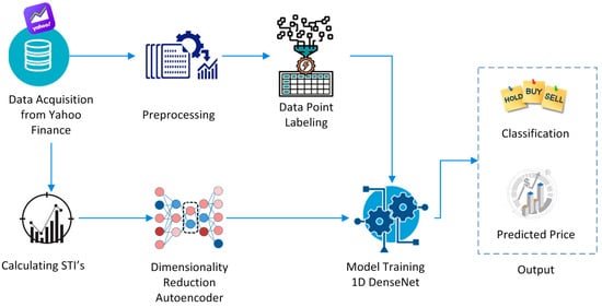
Figure 1.
Proposed methodology AEI-DNET.
3.1. Data Acquisition and Preprocessing
In this work, we took data of ten companies from a renowned financial web portal, namely, Yahoo Finance. For each stock, we took 2640 data points per trading day, where each datapoint comprised high and low prices, daily open and close values, paid dividends, trading volume, etc. After the data acquisition, we performed the data preprocessing step, which involved guessing the missing price values from the available adjacent price values via employing a linear regression approach. After gathering the data, we split it into two sets: the training and testing datasets.
3.2. Datapoints Labeling
Our work predicted the future stock prices by categorizing each stock into three classes: buy, hold, and sell. We assigned a class label to each data point based on the upcoming behavior of their closing prices and selected forecast horizon. Our work is based on a three-class classification problem, three types of labels, namely, ‘buy’ indicated as 10, ‘sell’ indicated as 01, and ‘hold’ indicated as 00, were assigned to each data point.
The labels were assigned by using the equation.
Here, d(t) is the initial day, while f(s) shows the selected forecast horizon. Moreover, and exhibit the closing prices on day d and d + f respectively, and δ indicates the threshold value. The label ‘buy’ is assigned to a datapoint if the related closing stock price goes up from the selected threshold, a data point is labeled as ‘sell’ if the corresponding closing stock price goes down from the selected threshold, and a data point is assigned as ‘hold’ if the change in the stock price remains between the negative and positive thresholds. The threshold value presents a slight relative change in the stock price, i.e., its rise or fall, which can be considered a directional movement [18]. Various chosen threshold values for our work over numerous forecast horizons are demonstrated in Table 1. The value of the threshold was selected so that each class contains about one-third of the data points. Moreover, the value of the threshold rises with the increase in the horizon as the price value also increases with time, which needs a large threshold number to put one-third of the data points into the ‘hold’ class.

Table 1.
Horizon with thresholds.
3.3. Stock Technical Indicators
Stock technical indicators are statistical features of stock data calculated by incorporating various mathematical formulas to establish a fair estimation of prices and volumes. Some of the most used technical indicators are various variants of a moving average, momentum oscillators, and various flow indices. The following subsections provide a brief description of each STI incorporated in our work.
3.3.1. Simple Moving Average (MA)
A common STI presents the price average over a selected range, mostly containing closing prices (Cp), using the total number of days in that range [20].
3.3.2. Weighted Moving Average (WMA)
This STI is used to generate the trade direction and make a buy or sell decision [34]. The WMA is calculated by multiplying each data observation by a predetermined weighting factor, which is described as
Here, Cp is the closing price each day over N days.
3.3.3. Exponential Moving Average (EA)
This STI is an enhanced form of the WMA, giving more importance to recent price data. It is used to track the stock prices at a specific time interval [35].
where is equal to 1.
3.3.4. Relative Strength Index (RSI)
It provides a comparison of the current gains with losses. The main aim of this indicator is to show the ups and downs in the price trends of stock by considering its closing prices in a specified time interval [36]. The mathematical representation of STI computation is given by
where EAn(DM+ve) and EAn(DM−ve) are calculated over a time interval of the N previous days equal to the IWL.
3.3.5. Chande Momentum Oscillator (CMO)
The CMO is another well-known STI that employs momentum to locate the relative behavior of stock by demonstrating its strengths and weaknesses in a particular period [37]. The CMO is computed using
Here, for N days, the Sh and Sl are the summations of the higher and lower closes.
3.3.6. Williams Percent Range (Williams %R)
This STI is used to measure the overbought and oversold levels and to identify the entry and exit points in the market using the following equation [18]:
Here, Cp is closed price, and HN and LN show the high and low prices over N days, respectively.
3.3.7. Price Rate of Change (PRC)
This STI is used to demonstrate the correlated differences between the Cp on forecasted data and the Cp computed on N previous days [38]. The PRC is given by
3.3.8. Hull Moving Average (HMA)
The HMA is a directional trend indicator that captures the current state of the market by using the recent price action to determine whether conditions are bullish or bearish [39]. The HMA is computed using
3.3.9. Triple Exponential Moving Average (TEA)
This STI smoothens the price fluctuation to make the trend identification easier, without the lag associated with the MA [40].
where .
3.3.10. Directional Movement Index (DMI)
This STI identifies the direction of price movement by comparing prior highs and lows [41].
where , , , and .
3.3.11. Psychological Line (PL)
This STI indicates the buying capability compared to selling by showing the fraction of numbers of rising days with the total days.
3.3.12. Commodity Channel Index (CCI)
This STI is employed to check the strength and trend direction of stocks, which can assist the buyers in decision making to avail a trade opportunity or not and to hold on to an existing trade [42]. The CCI is computed using
Here, Ts is the total sum of the closing high and low prices on day s. Moreover, the MAN is the MA of Ts calculated for N days.
3.3.13. Chaikin Money Flow Index (CMF)
This STI indicates the difference between the 3-day EA and the 10-day EA of the accumulation/distribution line [43].
3.3.14. Moving Average Convergence Divergence (MAD)
This is another influential STI that shows the relationship between two running averages of stock prices [44]. This STI is calculated by taking the difference of the EA of 26 days from the EA of 12 days.
3.3.15. Stochastic Oscillator %K (SO)
The SO indicator [45] shows the comparison of a specific closing price of a stock to a range of its prices for a specific period T and determines whether a stock is highly sold or bought, as given in the following equation:
Here, HM and LM are the mean highest high and low values over N days, respectively.
3.3.16. Moving Average Deviation (MD)
The MD indicator shows the deviation in price from the moving average (MA), and the computed deviated value is shown by histogram bars [46]. The mathematical calculation of MD is done using the following equation:
3.3.17. Rank Correlation Index (RCI)
The RCI indicator [47] is used to identify potential changes in market sentiment to expose turning points. RCI is the combination of price change data and time change data, which is given in the following equation:
3.3.18. Bollinger Bands (BB)
The BB STI [48] is a powerful indicator of stock market prediction that enables investors to properly identify the time when an asset is oversold or overbought. The mathematical description of BB is given as
3.4. Dimensionality Reduction
Once the STIs were calculated, the next step was to reduce the dimensions of the data features. This step is important in the sense that it helps reduce the required time for model training and storage space requirements. It helps remove multi-collinearity, which improves the interpretation of the parameters of the model. A model with very low dimensions is generally easier to train; it is also easier to visualize the output data.
Autoencoder
Despite the usage of DenseNet results in an efficient set of STI representations, the data still suffered from a high dimensional space. To deal with this issue, we employed the autoencoder technique. Autoencoder networks are feedforward NNs that can contain more than one hidden layer. This approach tends to reconstruct the input data to reduce the dimensions of input samples.
In an autoencoder [49], the input and output layers have similar dimensions; however, the hidden layers have different data dimensions since the data reduction occurs here. The encoder takes and compressed it to in the hidden layers via employing an activation function f(x) given by the following equation:
Here, W is a weight matrix.
The encoding process is achieved using the following equation:
while the decoding process is achieved using the following equation:
Here, g() is an activation function similar to f(x), and is another weighted matrix. Furthermore, denotes the decoded compressed input string.
The autoencoder computes the total reconstruction error for all samples using the following equation:
where is the weighted reconstruction error for an individual sample.
3.5. Model Training
After calculating the STIs, we used them as the autoencoder input for dimensionality reduction and a reduction in correlation among STIs. For this purpose, we used the 1D DenseNet framework instead of 2D vectors because of the textual nature of our dataset.
1D DenseNet
The 1D DenseNet framework was used for deep features extraction in the presented approach. The main reason to select the DenseNet framework over the ResNet approach is that, although the ResNet network is capable of dealing with the problem of vanishing gradient descent to some extent, the ResNet approach is computationally complex, as the network parameters increase exponentially with the increase in the depth of architecture. In contrast, DenseNet can better overcome the issues of the ResNet approach by introducing densely connected CNNs. Therefore, the main motivation for using the DenseNet framework is to present an efficient and effective solution for stock price prediction.
The DenseNet framework comprises a dense block, which is a transition layer along with the bottleneck layer. The architecture of the DenseNet framework is presented in Figure 2, where it can be seen that it consists of an (N − 1)-layered network and a composite function (CF). The CF further contains ReLU, batch normalization, and the convolution function. More specifically, the input data from the Yahoo Finance dataset was passed to the 1D DenseNet framework for feature computation. The convolution layers computed the deep features from the sample data by using a kernel window size of 3. The entire DenseNet framework contained four dense blocks, with each block comprising four convolution layers. Furthermore, each convolution layer applied four methods named batch normalization, ReLU activation, and squeeze and excite operations, as discussed in [50]. Initially, the number of filters was set to 32 and increased by 16 after each step, which, in turn, caused an increase in the feature vector size due to the concatenation operation. The transition layer was introduced after each DB to perform the down-sampling step to deal with this.
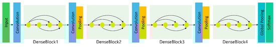
Figure 2.
Architecture of the 1D DenseNet framework.
The Nth layer of the framework had N inputs, as the Nth layer took the outputs of all previous N − 1 layers, as seen in Equation (26):
Here, are the feature maps from the previous N − 1 layers, which were joined to the Nth layer and indicated by .
Furthermore, the transition layer comprised convolution and pool layers. The bottleneck layer contained a 1 × 1 convolution layer, which was employed to minimize the size of feature maps and enhance computational efficiency.
4. Experimental Results
This section provides a detailed overview of the incorporated dataset, performed experiments, and evaluation parameters used for the evaluation of the experimental results. The model was implemented using the Python platform. The proposed technique was further evaluated by providing a comparative analysis with other models as well.
4.1. Dataset
This research work incorporated publicly available historical financial stock market data available at Yahoo Finance. The historical financial data obtained from the said platform has a total of seven columns containing Date, Open, High, Low, Close, Adj Close, and Volume. Description of these attributes is provided in Table 2.
Table 2.
Description of the historical stock dataset.
Additionally, we also calculated H − L (stock high minus low price) and O − C (stock open minus close price) for calculation purposes. Moreover, we also calculated some important stock technical indicators (STIs) and used them as input features for training the model. A detailed discussion regarding STIs was already done in the previous section. The dataset under consideration consisted of the ten previous years’ financial records of ten different stocks. Detail of the stocks and dataset is provided in Table 3. We took the historical stock price data and STIs as input to the training model. We selected the Standard and Poor’s 500 index series (S&P 500) as the base time-series measure related to financial time-series data. This series was built using the Yahoo Finance data posted over the past ten years. The information gained from this series served as the base for calculating the technical indicators and the target output, and the same was used as input into the training model. We created binary variables to indicate the expected output related to the target output. The value 10 indicated that the closing price was expected to go up compared with the closing price during the current day, meaning that the model shall indicate a buy signal. Similarly, the value 01 indicated that the close price was expected to go down the next day compared with the closing price reported on the current day, meaning that the model shall indicate a sell signal. Similarly, a 00 signal indicated that no significant short-term change in the closing price was expected, meaning that the model shall indicate a sell signal.
Table 3.
Brand-wise distribution of the dataset.
We present a case study based on the S&P 500 with ten US stocks: FB, TWTR, INTC, AAPL, MSFT, GOOG, TSLA, WMT, AMZN, and PYPL. As discussed earlier, we obtained ten years of stock trading data from Yahoo Finance posted during the past ten years, i.e., from 1 October 2011 to 30 September 2021 (subject to availability). The experimental data consisted of daily trade information including LO, HI, OP, CL, AD, and VO, representing low, high, opening price, closing price, adjusted close price, and volume.
For the sake of understanding, Figure 3 presents a visualization of the dataset distribution. Trading data for all stocks were divided into two parts, i.e., training and testing data with a 30%:70% ratio (approximately), resulting in 1760 trading days’ data for training and 756 trading days’ data for testing purposes, except for FB and TWTR, as these stocks started posting their stock data from 19 May 2012 and 11 July 2013, respectively. This resulted in 1601 and 1316 trading days’ data for FB and TWTR, respectively. We suspect that a relatively lower amount of training data for these two stocks may slightly affect the model performance.
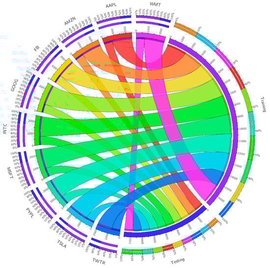
Figure 3.
A visualization of dataset distribution.
4.2. Evaluation Parameters
We measured the reliability of the experimental results by incorporating several criteria, including the mean absolute error (MAE), root mean square error (RMSE), mean absolute percentage error (MAPE), average mean absolute percentage error (AMAPE), and percentage of correct trend (PCT). The first performance metric, i.e., MAE was presented in, where it is a commonly used approach in forecasting; it can be calculated using Equation (27). The RMSE can be calculated using Equation (28). The third performance evaluation parameter was MAPE, which was used to calculate the percentage error between the actual and predicted values. MAPE is described using Equation (29). The next parameter, i.e., AMAPE is given in Equation (30). Finally, the metric named PCT is used to evaluate the accuracy of predicted ups and downs and can be calculated using Equation (31).
where denotes the actual value, denotes the predicted value, and a total number of data points is represented by .
4.3. Experimental Results
The utility of our proposed system was demonstrated by testing six models: autoregressive moving average (ARMA), generalized autoregressive conditional heteroskedasticity (GARCH), support vector machine (SVM), feed-forward neural network (FFNN), long short-term memory (LSTM), and the proposed 1D DenseNet. The value to be predicted was the closing price of the next day. We performed predictive experiments using Anaconda (Python), TensorFlow, and scikit-learn packages. There are various approaches for feeding the input variables into the model. The basic stock trading data (LO, HI, OP, CL, AD, and VO) were fed into the above-mentioned models as the input variables. Talking about the models, LSTM used four variations of input method: LSTIM-I, LSTIM-II, LSTIM-III, and LSTIM-IV. The LSTIM-I used the basic trading data. LSTIM-II took the trading data and technical indicators after being processed by the autoencoder. LSTIM-III took the trading data and technical indicators after all variables were processed by autoencoder. LSTIM-I and LSTIM-III did not involve any processing by the autoencoder. LSTIM-IV and the proposed 1D DenseNet took the trading data and technical indicators after processing only the STIs by the autoencoder.
These variations in the input method of LSTM are depicted in Figure 4. The first experiment aimed to predict the next day’s closing price in the S&P 500. The experiment mainly involved four variations of test data: 75 days for short-term prediction, 150 days for medium-term prediction, and 300 days for long-term prediction. For each type of test, the remaining data were used as training data. The experimental results obtained from the short-, medium-, and login-term trading data are presented in Table 4, Table 5, Table 6, Table 7, Table 8, Table 9, Table 10, Table 11, Table 12, Table 13, Table 14, Table 15, Table 16, Table 17 and Table 18. It is evident from the results that our proposed model had better accuracy compared with other models while predicting the closing price for short-, medium-, and long-term trading data. It is obvious that our model had the best performance regarding RMSE, MAPE, MAE, and AMAPE, which had the smallest values, and PCT, which had the highest values.
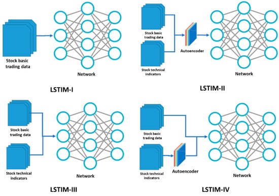
Figure 4.
Different input methods for the LSTM.
Table 4.
Prediction performance for 75 days: FB and TWTR.
Table 5.
Prediction performance for 75 days: INTC and AAPL.
Table 6.
Prediction performance for 75 days: MSFT and GOOG.
Table 7.
Prediction performance for 75 days: TSLA and WMT.
Table 8.
Prediction performance for 75 days: AMZN and PYPL.
Table 9.
Prediction performance for 150 days: FB and TWTR.
Table 10.
Prediction performance for 150 days: INTC and AAPL.
Table 11.
Prediction performance for 150 days: MSFT and GOOG.
Table 12.
Prediction performance for 150 days: TSLA and WMT.
Table 13.
Prediction performance for 150 days: AMZN and PYPL.
Table 14.
Prediction performance for 300 days: FB and TWTR.
Table 15.
Prediction performance for 300 days: INTC and AAPL.
Table 16.
Prediction performance for 300 days: MSFT and GOOG.
Table 17.
Prediction performance for 300 days: TSLA and WMT.
Table 18.
Prediction performance for 300 days: AMZN and PYPL.
It was also evident from the results that the fourth input method of LSTM, i.e., LSTIM-IV, had the overall second-best performance regarding MAPE, AMAPE, MAE, RMSE, and PCT. This was due to the involvement of the autoencoder for the dimensionality reduction of STIs before forwarding to the model.
Pictorial representations of the comparison between the predictive result and actual values are presented in Figure 5, Figure 6, Figure 7, Figure 8 and Figure 9 in the form of time-series charts. These charts show the performance on the testing data of 75, 150, and 300 trading days, respectively.
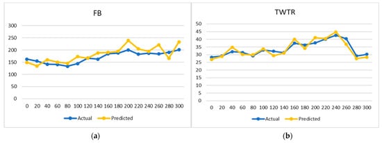
Figure 5.
Price predicting graph for (a) FB and (b) TWTR.
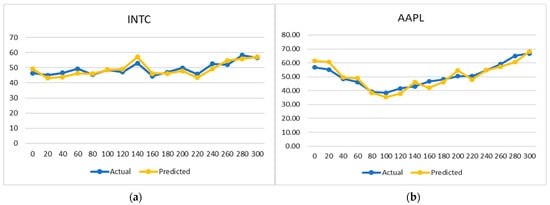
Figure 6.
Actual and predicted price graph for (a) INTC and (b) AAPL.
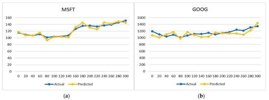
Figure 7.
Future price estimation graph (a) MSFT and (b) GOOG.
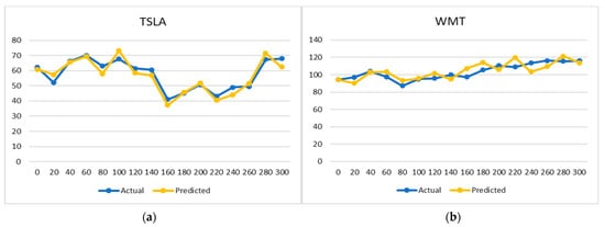
Figure 8.
Stock trend prediction for (a) TSLA and (b) WMT.
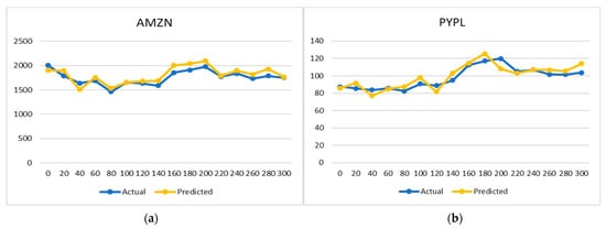
Figure 9.
Future Price determination for (a) AMZN and (b) PYPL.
Closer predicted results to the actual line present a more accurate prediction. The performance of the proposed model regarding accuracy is presented in Figure 5, Figure 6, Figure 7, Figure 8 and Figure 9. Additionality, an accuracy timeline for 300 trading days is presented in Figure 10. As expected, the model performance for the stock named FB was slightly degraded due to fewer training data for the said stock. As discussed earlier, this slight degradation in model training for the said class was due to the fact that FB and TWTR started appearing in the US stock markets from May 2012 and July 2013, respectively.
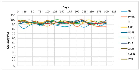
Figure 10.
Accuracy timeline.
Although the short-term and medium-term predictions in stock data are more desirable in the stock market, the long-term prediction is also significant, as a prediction of the direction of stock prices is normally more important for value investing in the long term, resulting in wiser decisions in the short- and medium-term perspectives. For the classification part, the trained model provides suggestions to the investor using one of the three signals, i.e., buy, hold, and sell, depending on the short-, medium-, and long-term stock trends under consideration. For instance, if the prices are expected to go up in the short- and medium-term, the model may generate a buy signal. Similarly, if the prices are expected to go up in the short term but they are expected to go down in the medium- and long-term, the model may generate a sell signal. Finally, if the prices are expected to go down in the short term but are expected to go up in the medium term, then the model may generate a hold signal. Again, the above scenario is just an example scenario, and it is presented only for the sake of understanding. The model may generate a signal purely based on short-, long-, and medium-term stock trends.
4.4. Comparison with ML-Based Methods
In this section, we compare our results against well-known ML-based approaches, namely, random forest, gradient boosting, and XGBoost, where the obtained results are reported in Table 19. We compared the approaches both in terms of precision results and computational time. It is quite clear from Table 19 that our approach was more robust regarding stock market prediction, both in terms of forecasting and computational complexity. More specifically, the random forest approach showed the lowest prediction results with MAPE and MAE values of 3.18 and 54.06, respectively, along with the execution time of 1.316 ms. Meanwhile, the second-lowest values were acquired by the gradient boosting approach, with the MAPE and MAE scores of 2.54 and 43.59, respectively, with the execution time of 1.483 ms. In comparison, the proposed approach attained MAPE and MSE values of 0.41 and 8.12, respectively, with an execution time of 1.051 ms. The main reason for our approach’s better stock prediction performance was its more accurate feature extraction power, which improved its recognition ability.
Table 19.
Comparison with ML-based methods.
4.5. Comparison with Other Techniques
In this section, we present the comparison of our technique with other existing methods using the same dataset. To demonstrate the performance comparison, we accomplished the comparative analysis by comparing our methods through metrics, namely, MAPE and MAE, with the reported results of the approaches [1,49,50,51]. The comparative results are given in Table 20. The reason for selecting the MAPE and MAE evaluation metrics was that researchers heavily explore these to demonstrate the stock prediction performance of the models. It is quite clear from the results reported in Table 20 that our work was more robust regarding stock market future trends predictions, as it shows lower MAPE and MAE values in comparison to the other latest approaches stated in [1,49,50,51]. The main reason for the better performance of the proposed solution was due to the reliable feature extraction power of the 1D DenseNet, which presents the complex price transformations in a viable manner. In comparison, the competitor approaches [1,51] deploy very complex network architectures, which causes the production of over-fitted training data, ultimately reducing their performance. Therefore, it can be said that our work is more effective regarding stock market prediction.
Table 20.
Comparison with state-of-the-art approaches.
4.6. Discussion
Stock trends prediction is an important topic of research and a challenging one due to the volatile, diverse, and dynamic nature of the stock market. Studies presented in recent years have revealed that STIs are a significant set of predictors for stock market future price estimation. However, the selection of more suitable STIs becomes a challenging task, as highly correlated STIs do not perform well in reliable feature extraction. To deal with the mentioned challenges, we presented a novel approach that employed both the STIs and stock data to make the final prediction. The main novelty of this work is that we are employing both STIs and finance data with a DL-based framework, which results in computing a more representative set of stock features. The evaluation results confirmed that the proposed approach attained robust prediction performance with reduced computational complexity. Therefore, we can say that our work can assist the business community in making timely beneficial decisions. The following are the advantages and limitations of our proposed method.
4.6.1. Advantages
- A novel framework employs STIs and stock data to predict future stock trends.
- Computationally efficient, as we employed an autoencoder framework for dimensionality reduction.
- A robust approach that can assist the business community in making timely beneficial decisions.
- The proposed approach predicts stock trends and provides intelligent decisions to hold, buy, or sell a product.
- Our method’s processing or prediction time was 1.051 ms, which is remarkable.
- Proposed a novel approach that opened a new research area in the field of natural language processing or text analysis.
4.6.2. Limitations
- The model needs evaluation on an unseen database to show its generalization ability better.
- This study is currently limited to the US stock market only. Therefore, a more generalized model shall enable us to include other stock markets, such as the Asian and European stock markets.
- More DL-based frameworks can be tested with the employed technique to enhance the prediction accuracy further.
5. Conclusions
Stock market price prediction is a challenging and interesting task regarding financial, scientific, and academic research. Recent developments in machine learning, especially DL, have made it possible to predict future stock price trends based on historical events. Advanced machine learning algorithms have enabled researchers to use intelligent methods to predict stock prices based on social media posts, financial news, and stock technical indicators (STIs). The main focus of this work is to predict the stock market prices by using STIs and stock market data, such as daily closing prices.
As already mentioned, this work focuses on predicting the stock market closing prices based on the STIs by using 1D DenseNet, followed by dimensionality reduction using an autoencoder. We first gathered ten years of financial stock trading data from Yahoo Finance, then calculated eighteen STIs from these data and then fed these STIs, along with the stock trading data, into the 1D DenseNet model after dimensionality reduction of the STIs from the autoencoder. Finally, the computed feature set obtained from the 1D DenseNet framework was used as input for training the softmax layer residing in the 1D DenseNet framework for short-, medium-, and long-term prediction of the closing stock prices. Although the prediction of short- and medium-term predictions in stock data are more desirable in the stock market, the long-term prediction is also significant as a prediction of the direction of stock prices and is normally more important for value investing in the long term, resulting in wiser decisions in short- and medium-term perspectives. Based on the predicted trends of the stock prices, our model provides suggestions to the user using one of three signals, i.e., buy, sell, or hold.
This research focused on predicting the stock prices of US stock markets. We aim to extend this study to Asian and European stock markets in the future. Additionally, this study was limited to the prediction of closing prices at daily intervals. We are investigating the possibility of predicting the stock price fluctuation on a time interval shorter than one day. This investigation will require more fine-grained historical stock market data, which was unavailable in the current dataset. This task demands implementing a separate investigation and a different set of experiments, which can be considered future work.
Author Contributions
Conceptualization, Formal Analysis, Data Analysis, Data Interpretation, Literature Search, Funding Acquisition, Project Administration, S.A.; Conceptualization, Software, Resources, Methodology, Writing—Original draft, T.N.; Validation, Visualization, Writing—Original draft, A.M.; Developed the contextualization of the state of the art, Supervision, Validation, Writing—review and editing. A.I.; Literature Search, Investigation, Validation, A.A.; Conceptualization, Supervision, Writing—review and editing, proofreading, W.A. All authors have read and agreed to the published version of the manuscript.
Funding
This research was funded by the Deanship of Scientific Research, Qassim University under the number (10302-coc-2020-1-3-I) during the academic year 1441 AH/2020 AD.
Acknowledgments
The authors gratefully acknowledge Qassim University, represented by the Deanship of Scientific Research, for the financial support for this research under the number 10302-coc-2020-1-3-I during the academic year 1441 AH/2020 AD.
Conflicts of Interest
The authors declare no conflict of interest.
References
- Nabipour, M.; Nayyeri, P.; Jabani, H.; Mosavi, A.; Salwana, E. Deep learning for stock market prediction. Entropy 2020, 22, 840. [Google Scholar] [CrossRef]
- Asadi, S.; Hadavandi, E.; Mehmanpazir, F.; Nakhostin, M.M. Hybridization of evolutionary Levenberg–Marquardt neural networks and data pre-processing for stock market prediction. Knowl.-Based Syst. 2012, 35, 245–258. [Google Scholar] [CrossRef]
- Akhter, S.; Misir, M.A. Capital markets efficiency: Evidence from the emerging capital market with particular reference to Dhaka stock exchange. South Asian J. Manag. 2005, 12, 35. [Google Scholar]
- Miao, K.; Chen, F.; Zhao, Z.G. Stock price forecast based on bacterial colony RBF neural network. J. Qingdao Univ. (Nat. Sci. Ed.) 2007, 2, 11. [Google Scholar]
- Lehoczky, J.; Schervish, M. Overview and history of statistics for equity markets. Annu. Rev. Stat. Its Appl. 2018, 5, 265–288. [Google Scholar] [CrossRef]
- Hoseinzade, E.; Haratizadeh, S. CNNpred: CNN-based stock market prediction using a diverse set of variables. Expert Syst. Appl. 2019, 129, 273–285. [Google Scholar] [CrossRef]
- Jiang, W. Applications of deep learning in stock market prediction: Recent progress. Expert Syst. Appl. 2021, 115537. [Google Scholar] [CrossRef]
- Weng, B.; Ahmed, M.A.; Megahed, F.M. Stock market one-day ahead movement prediction using disparate data sources. Expert Syst. Appl. 2017, 79, 153–163. [Google Scholar] [CrossRef]
- Bustos, O.; Pomares-Quimbaya, A. Stock market movement forecast: A Systematic review. Expert Syst. Appl. 2020, 156, 113464. [Google Scholar] [CrossRef]
- Shah, D.; Isah, H.; Zulkernine, F. Stock market analysis: A review and taxonomy of prediction techniques. Int. J. Financ. Stud. 2019, 7, 26. [Google Scholar] [CrossRef] [Green Version]
- Olivas, E.S.; Guerrero, J.D.M.; Martinez-Sober, M.; Magdalena-Benedito, J.R.; Serrano, L. Handbook of Research on Machine Learning Applications and Trends: Algorithms, Methods, and Techniques; IGI Global: Hershey, PA, USA, 2009; ISBN 1605667676. [Google Scholar]
- Aldin, M.M.; Dehnavi, H.D.; Entezari, S. Evaluating the employment of technical indicators in predicting stock price index variations using artificial neural networks (case study: Tehran Stock Exchange). Int. J. Bus. Manag. 2012, 7, 25. [Google Scholar]
- Tsai, C.-F.; Lin, Y.-C.; Yen, D.C.; Chen, Y.-M. Predicting stock returns by classifier ensembles. Appl. Soft Comput. 2011, 11, 2452–2459. [Google Scholar] [CrossRef]
- Corbet, S.; Eraslan, V.; Lucey, B.; Sensoy, A. The effectiveness of technical trading rules in cryptocurrency markets. Financ. Res. Lett. 2019, 31, 32–37. [Google Scholar] [CrossRef]
- Sezer, O.B.; Ozbayoglu, A.M. Algorithmic financial trading with deep convolutional neural networks: Time series to image conversion approach. Appl. Soft Comput. 2018, 70, 525–538. [Google Scholar] [CrossRef]
- Sobolev, D.; Chan, B.; Harvey, N. Buy, sell, or hold? A sense-making account of factors influencing trading decisions. Cogent Econ. Financ. 2017, 5, 1295618. [Google Scholar] [CrossRef]
- Liang, D.; Tsai, C.-F.; Lu, H.-Y.R.; Chang, L.-S. Combining corporate governance indicators with stacking ensembles for financial distress prediction. J. Bus. Res. 2020, 120, 137–146. [Google Scholar] [CrossRef]
- Shynkevich, Y.; McGinnity, T.M.; Coleman, S.A.; Belatreche, A.; Li, Y. Forecasting price movements using technical indicators: Investigating the impact of varying input window length. Neurocomputing 2017, 264, 71–88. [Google Scholar] [CrossRef] [Green Version]
- Chun, D.; Cho, H.; Ryu, D. Economic indicators and stock market volatility in an emerging economy. Econ. Syst. 2020, 44, 100788. [Google Scholar] [CrossRef]
- Dai, Z.; Dong, X.; Kang, J.; Hong, L. Forecasting stock market returns: New technical indicators and two-step economic constraint method. N. Am. J. Econ. Financ. 2020, 53, 101216. [Google Scholar] [CrossRef]
- Fayek, M.B.; El-Boghdadi, H.M.; Omran, S.M. Multi-objective optimization of technical stock market indicators using gas. Int. J. Comput. Appl. 2013, 68, 41–48. [Google Scholar]
- Maguluri, L.P.; Ragupathy, R. An Efficient Stock Market Trend Prediction Using the Real-Time Stock Technical Data and Stock Social Media Data. Int. J. Intell. Eng. Syst. 2020, 13, 316–332. [Google Scholar] [CrossRef]
- Zhang, J.; Li, L.; Chen, W. Predicting stock price using two-stage machine learning techniques. Comput. Econ. 2021, 57, 1237–1261. [Google Scholar] [CrossRef]
- Agrawal, M.; Khan, A.U.; Shukla, P.K. Stock indices price prediction based on technical indicators using deep learning model. Int. J. Emerg. Technol. 2019, 10, 186–194. [Google Scholar]
- JuHyok, U.; Lu, P.; Kim, C.; Ryu, U.; Pak, K. A new LSTM based reversal point prediction method using upward/downward reversal point feature sets. Chaos Solitons Fractals 2020, 132, 109559. [Google Scholar]
- Yang, C.; Zhai, J.; Tao, G. Deep learning for price movement prediction using convolutional neural network and long short-term memory. Math. Probl. Eng. 2020, 2020, 2746845. [Google Scholar] [CrossRef]
- Lee, J.W. Stock price prediction using reinforcement learning. In Proceedings of the 2001 IEEE International Symposium on Industrial Electronics Proceedings (Cat. No. 01TH8570), Pusan, Korea, 12–16 June 2001; IEEE: Piscataway, NJ, USA, 2001; Volume 1, pp. 690–695. [Google Scholar]
- Gu, Y.; Yan, D.; Yan, S.; Jiang, Z. Price forecast with high-frequency finance data: An autoregressive recurrent neural network model with technical indicators. In Proceedings of the 29th ACM International Conference on Information & Knowledge Management, Online, 19–23 October 2020; pp. 2485–2492. [Google Scholar]
- Chiewhawan, T.; Vateekul, P. Explainable deep learning for thai stock market prediction using textual representation and technical indicators. In Proceedings of the 8th International Conference on Computer and Communications Management, Singapore, 17–19 July 2020; pp. 19–23. [Google Scholar]
- Vargas, M.R.; dos Anjos, C.E.M.; Bichara, G.L.G.; Evsukoff, A.G. Deep leaming for stock market prediction using technical indicators and financial news articles. In Proceedings of the 2018 International Joint Conference on Neural Networks (IJCNN), Rio de janeiro, Brazil, 8–13 July 2018; IEEE: Piscataway, NJ, USA, 2018; pp. 1–8. [Google Scholar]
- Wu, J.M.-T.; Li, Z.; Herencsar, N.; Vo, B.; Lin, J.C.-W. A graph-based CNN-LSTM stock price prediction algorithm with leading indicators. Multimed. Syst. 2021, 1–20. [Google Scholar] [CrossRef]
- Adebiyi, A.A.; Ayo, C.K.; Adebiyi, M.; Otokiti, S.O. Stock price prediction using neural network with hybridized market indicators. J. Emerg. Trends Comput. Inf. Sci. 2012, 3, 1–9. [Google Scholar]
- Yıldırım, D.C.; Toroslu, I.H.; Fiore, U. Forecasting directional movement of Forex data using LSTM with technical and macroeconomic indicators. Financ. Innov. 2021, 7, 1. [Google Scholar] [CrossRef]
- Hunter, J.S. The exponentially weighted moving average. J. Qual. Technol. 1986, 18, 203–210. [Google Scholar] [CrossRef]
- Lawrance, A.J.; Lewis, P.A.W. An exponential moving-average sequence and point process (EMA1). J. Appl. Probab. 1977, 14, 98–113. [Google Scholar] [CrossRef]
- Ţăran-Moroşan, A. The relative strength index revisited. Afr. J. Bus. Manag. 2011, 5, 5855–5862. [Google Scholar]
- Di Lorenzo, R. Other Oscillators. In Basic Technical Analysis of Financial Markets; Springer: Berlin/Heidelberg, Germany, 2013; pp. 189–220. [Google Scholar]
- Seker, S.E.; Cihan, M.; Khaled, A.-N.; Ozalp, N.; Ugur, A. Time series analysis on stock market for text mining correlation of economy news. Int. J. Soc. Sci. Humanit. Stud. 2013, 6, 69–91. [Google Scholar]
- Letchford, A.; Gao, J.; Zheng, L. Optimizing the moving average. In Proceedings of the 2012 International Joint Conference on Neural Networks (IJCNN), Brisbane, Australia, 10–15 June 2012; IEEE: Piscataway, NJ, USA, 2012; pp. 1–8. [Google Scholar]
- Raudys, A.; Lenčiauskas, V.; Malčius, E. Moving averages for financial data smoothing. In Proceedings of the International Conference on Information and Software Technologies, Kaunas, Lithuania, 10–11 October 2013; Springer: Berlin/Heidelberg, Germany, 2013; pp. 34–45. [Google Scholar]
- Lam, W.-S.; Chong, T.T.-L. Profitability of the directional indicators. Appl. Financ. Econ. Lett. 2006, 2, 401–406. [Google Scholar] [CrossRef]
- Maitah, M.; Procházka, P.; Cermak, M.; Šrédl, K. Commodity channel index: Evaluation of trading rule of agricultural commodities. Int. J. Econ. Financ. Issues 2016, 6, 176–178. [Google Scholar]
- Thomsett, M.C. CMF--Chaikin Money Flow: Changes Anticipating Price Reversal; FT Press: Upper Saddle River, NJ, USA, 2010; ISBN 0132492067. [Google Scholar]
- Hung, N.H. Various moving average convergence divergence trading strategies: A comparison. Invest. Manag. Financ. Innov. 2016, 13, 363–369. [Google Scholar] [CrossRef]
- Markus, L.; Weerasinghe, A. Stochastic oscillators. J. Differ. Equ. 1988, 71, 288–314. [Google Scholar] [CrossRef] [Green Version]
- Halimawan, A.A.; Sukarno, S. Stock Price Forecasting Accuracy Analysis using Mean Absolut Deviation (MAD) and Mean Absolute Percentage Error (MAPE) on Smoothing Moving Average and Exponential Moving Average Indicator (Empirical Study 10 LQ 45 Stock with Largest Capitalization from pe. Indones. J. Bus. Adm. 2013, 2, 68283. [Google Scholar]
- Hernández-Aguirre, A.; Villa-Diharce, E.; Barba-Moreno, S. An estimation distribution algorithm with the spearman’s rank correlation index. In Proceedings of the 10th Annual Conference on Genetic and Evolutionary Computation, Atlanta, GA, USA, 12–16 July 2008; pp. 469–470. [Google Scholar]
- Bollinger, J. Using bollinger bands. Stock. Commod. 1992, 10, 47–51. [Google Scholar]
- Kowsari, K.; Jafari Meimandi, K.; Heidarysafa, M.; Mendu, S.; Barnes, L.; Brown, D. Text classification algorithms: A survey. Information 2019, 10, 150. [Google Scholar] [CrossRef] [Green Version]
- Azar, J.; Makhoul, A.; Couturier, R. Using DenseNet for IoT multivariate time series classification. In Proceedings of the 2020 IEEE Symposium on Computers and Communications (ISCC), Rennes, France, 7–10 July 2020; IEEE: Piscataway, NJ, USA, 2020; pp. 1–6. [Google Scholar]
- Chung, H.; Shin, K. Genetic algorithm-optimized long short-term memory network for stock market prediction. Sustainability 2018, 10, 3765. [Google Scholar] [CrossRef] [Green Version]
- Lu, W.; Li, J.; Wang, J.; Qin, L. A CNN-BiLSTM-AM method for stock price prediction. Neural Comput. Appl. 2021, 33, 4741–4753. [Google Scholar] [CrossRef]
- Majumder, I.; Dash, P.K.; Bisoi, R. Short-term solar power prediction using multi-kernel-based random vector functional link with water cycle algorithm-based parameter optimization. Neural Comput. Appl. 2020, 32, 8011–8029. [Google Scholar] [CrossRef]
Publisher’s Note: MDPI stays neutral with regard to jurisdictional claims in published maps and institutional affiliations. |
© 2022 by the authors. Licensee MDPI, Basel, Switzerland. This article is an open access article distributed under the terms and conditions of the Creative Commons Attribution (CC BY) license (https://creativecommons.org/licenses/by/4.0/).