Explainable Computational Intelligence Model for Antepartum Fetal Monitoring to Predict the Risk of IUGR

Abstract

Intrauterine Growth Restriction (IUGR) is a restriction of the fetus that involves the abnormal growth rate of the fetus, and it has a huge impact on the new-born’s health. Machine learning (ML) algorithms can help in early prediction and discrimination of the abnormality of the fetus’ health to assist in reducing the risk during the antepartum period. Therefore, in this study, Random Forest (RF), Support Vector Machine (SVM), K Nearest Neighbor (KNN) and Gradient Boosting (GB) was utilized to discriminate whether a fetus was healthy or suffering from IUGR based on the fetal heart rate (FHR). The Recursive Feature Elimination (RFE) method was used to select the significant feature for the classification of fetus. Furthermore, the study Explainable Artificial Intelligence (EAI) was implemented using LIME and SHAP to generate the explanation and to add comprehensibility in the proposed models. The experimental results indicate that RF achieved the highest accuracy (0.97) and F1-score (0.98) with the reduced set of features. However, the SVM outperformed it in terms of Positive Predictive Value (PPV) and specificity (SP). The performance of the model was further validated using another dataset and found that it outperformed the baseline studies for both the datasets. The proposed model can aid doctors in monitoring fetal health and enhancing the prediction process.

1. Introduction

Each year 15 million babies are born around the world, and 11.4% of the pregnancies end up in early deliveries, which is around 1 in 10 [1]. Of these, 15–20% are medically indicated as having Preeclampsia, Intrauterine Growth Restriction (IUGR) or Abruption. Furthermore, babies born between 32–33 weeks have a 95% chance of survival, and these chances decrease along with the birth term down to a 17% chance for babies born in the 23rd week [2]. These chances of survival are associated with the complication of the born babies, and 20% of them might face temperature, breathing and feeding problems. Similarly, 5% most likely face development complications. Additionally, the delivery cost of premature baby is, on average, 7.4% higher when compared with the normal health newborn.

IUGR is a dangerous condition that occurs during pregnancy and that indicates that the fetus is growing slowly and weighs less than the 10% for gestational age. The weight and development of the neonatal depends on the number of gestational weeks [3]. Comparing IUGR fetuses’ weights to the healthy neonate helps to identify the critical point of Fetal Heart Rate (FHR) and when to intervene to maintain the newborn’s life [4]. Early analysis and monitoring of HR and prenatal (antepartum) data of the fetus will help the doctors take the necessary actions by intervening at the right time to prevent deaths of premature babies. Effective analysis of these significant parameters of premature babies will definitely increase the number of healthier babies and reduce the risk of further complications.

An automatic intelligent system based on artificial intelligence (AI), machine learning (ML) and deep learning (DL) has revolutionized the diagnostic process. The ML system has demonstrated the significant performance in various fields including health using different types of data, such as clinical data, X-ray, computerized tomography (CT) scan, cardiotocography (CTG), electromyography (EMG) and genomic data [5,6,7,8,9,10]. Notwithstanding the implication of ML models in healthcare, it also lacks comprehensibility and transparency and is considered a black box technique [11]. Consequently, it is necessary to develop a model with enhanced interpretability. Therefore, in the proposed study, EAI was used along with the ML techniques for early diagnosis of fetal health using FHR for Antepartum Fetal Monitoring (AFM) to classify the fetus as healthy or IUGR. A number of studies using ML and DL techniques in healthcare have been reported; however, very few of them used EAI [12].

This paper is organized as follows: Section 2 consists of literature reviews of related work; Section 3 consists of material and methods, including the dataset description and a description of the classifiers; Section 4 consists of experiments, results and discussion; finally, Section 5 contains the conclusion.

2. Review of Related Literatures

The use of FHR for AFM to predict fetal health is an important method adopted in clinical practice to preserve fetal well-being during gestation. In this section, we outline several studies that employ machine learning to classify the IUGR and healthy fetuses by using the FHR parameters.

Gurgen et al. [4] used Support Vector Machines (SVM) to explore the risks of IUGR, which is associated with fetal hypoxia, leading to fetal development disorders. In the study, IUGR was predicted in two stages: during the first stage by using indicators such as non-invasive Doppler pulsatility index (PI), resistance index (RI), middle cerebral artery (MCA), etc., analyzing them and then using SVM to classify the fetus as “reactive” or “non-reactive and/or fetal distress (FD)”. The second stage involved verifying the correctness of the diagnosis through a nonstress test (NST) tool. The model was tested using 44 preterm pregnancies, with and without IUGR. They found that features such as Doppler indicators PI, RI and MCA are significant in achieving the greatest accuracy (0.81), specificity (0.933), sensitivity (0.625) and positive predictive value (PPV) (0.862).

In addition, Signorini et al. [13] used several ML techniques such as Random Forest (RF), Classification Trees (CT), Logistic Regression (LR) and SVM for antepartum fetal monitoring and detected the pathology during pregnancy using physiology-based heart rate features. The dataset consisted of 60 IUGR and 60 healthy fetus and had time, frequency and non-linear parameters. Similarly, the models were trained with 11 cardiac rate features extracted from prenatal Cardiotocographic (CTG) recording. They found that RF and CT achieved the greatest accuracy (0.911).

Furthermore, another study [14] was conducted on children born under IUGR conditions to identify the latent risk clinical attribute. The dataset consisted of 41 IUGR (18 male) and 34 healthy (22 male). The features were collected through 24 h monitoring of blood pressure and the electrocardiogram (ECG). Moreover, the same features were collected 9 years after birth. Several classifiers, such as LR, Extreme Gradient Boosting (XGBoost) and SVM, were assembled, and these achieved 0.947 accuracy. The proposed model will help in predicting latent risks of IUGR children through monitoring the collected attributes during their development.

Similarly, Zhao et al. [15] study aimed to propose a system for computerized analysis of FHR signal to assist medical services in decision making. The proposed system extracted 47 features from a collection of (linear and nonlinear) domains: morphological, time and frequency. Three ML algorithms were used: DT, SVM and Adaptive Boosting (AdaBoost). To enhance the system’s performance, several feature selection methods were used: Mann–Whitney–Wilcoxon Statistical Test (ST) using the p-value as a difference determination; Principal Component Analysis (PCA). The data was obtained from CTU-UHB in the obstetrics ward at the University Hospital in Brno, Czech Republic, from 2009 until 2012. It comprises a subset, which includes 9164 intrapartum CTG recordings; out of these recordings, 552 CTG signals were selected. The results have proved that AdaBoost outperformed the other classifier. The selected feature using Mann–Whitney–Wilcoxon ST gave better results when compared to the original dataset, with an accuracy and sensitivity of 0.92. In conclusion, the results have shown the efficiency and effectiveness of the proposed solution, with a comprehensive analysis of FHR signal to assist the medical services in their decision-making through intelligent prediction. However, to the best of the authors’ knowledge, more features should be added to enhance the system’s performance level.

Furthermore, a study [16] was conducted with the aim of finding a limited set of parameters that could be used to identify the early recognition of IUGR fetuses. The data set was the FHR Signals of 120 women (60 IUGRs and 60 normal) during their pregnancy. Several classifiers, such as LR, Naïve Bayes (NB), SVM-RBF, SVM Linear and Classification trees, were used. The study achieved the highest accuracy (0.925) using LR and linear SVM. These results show that the method should be widely used in clinics for predicting IUGR Fetuses. Similarly, Comert and Kocamaz’s [17] study used several ML techniques, such as Artificial Neural Networks (ANN), SVM, Extreme Learning Machines (ELM), Radial Base Function Networks (RBFN) and RF. Their dataset was created by SisProto software and consisted of 2126 instances and 21 features. The FHR signals were classified as either normal or hypoxic. All algorithms showed acceptable performance level. However, ANN achieved more accurate and reliable performance, with a sensitivity of 0.997 and specificity of 0.97.

Moreover, Signorini and Magenes’ [18] study aimed to show and discuss the acquired outcomes from Normal and IUGR populations of fetuses based on the time series of the FHR signal analysis by using Phase Rectified Signal Analysis (PRSA) to identify indices that can reduce the risk of diseases early in the pregnancy duration. The dataset consisted of 122 subjects (61 healthy and 61 IUGR) between 32–35 weeks of pregnancy, and the parameters were STV, LTI, and delta. On the other hand, the ApEn and SampEn were both calculated and used as nonlinear indices with the Lempel Ziv parameter, which is used to recognize the patterns of the FHR signal. By using LR, the study achieved an accuracy of 0.925. There are several influential factors that affect FHR variability, and these may vary between linear and nonlinear, so that only the multivariate approach can improve the differentiation between the healthy and distressed fetuses.

Chaaban et al. [19] noted that one of the complications of Hypertensive Disorders of Pregnancy (HDP) is IUGR, which changes the behavior of features extracted from FHRs. The study aimed to extract a new set of kurtosis-based features and classical time-based features, such as Sample Entropy and Fuzzy Entropy, from the FHR signal. These features were used to discover their effect on HDP and IUGR. K-means and SVM algorithm were used on 50 IUGR and 50 normal pregnancies. The study found that kurtosis-based features and SVM achieved the highest specificity and precision (1) and a sensitivity of 0.67. Similarly, Moreira et al. [20] presented an analysis of ML methods that can assist in detection of the fetus problem, especially the low-birth-weight problem. DT, SVM, K Nearest Neighbor (KNN), Boosting, Bagging and subspace KNN algorithms were used. The dataset consisted of 104 pregnant women suffering from hypertensive disorder during the gestation. The study found that bagged tree algorithm is the best one when compared with the other algorithms; it achieved an accuracy of 0.849.

Krupa et al. [21] discussed an approach for FHR interpretation based on Empirical Mode Decomposition (EMD) and SVM to classify obtained FHR records as “at risk” or “normal”. The FHR records were obtained from 15 subjects and the dataset consisted of 90 randomly selected records of specific duration. These records were labeled as “normal” or “at risk” by specialized doctors. The proposed approach used EMD standard deviation as an input to SVM for the classification of FHR samples. The study achieved the geometric mean of 0.815 and the Kappa value was 0.684. This method has shown an acceptable level of validity to be implemented for the FHR classification signals. However, in order to obtain a significant clinical accurate result, the method requires validation on a larger dataset, as well as further investigation of the use of EMD and SVM classifying approaches for studying the effects of sampling rates on extracted features.

Similarly, Pini et al. [22] developed an SVM model to predict late IUGR using the FHR. The study was performed using the CTG of 160 healthy and 102 late IUGR-pregnant women. A radial-based kernel method was used in the SVM. However, the features were selected using the RFE method. In addition to the feature extracted from the CTG, they also considered some additional features, such as GA, maternal age and the fetal gender. As a result of the non-availability of the fetus gender in most of the countries they performed experiments with and without the fetus gender. However, no significant difference appeared between this and the outcome of the classifier performance during the two previously mentioned experiments. They have achieved the highest accuracy (0.84), a sensitivity of 0.843 and a specificity of 0.85.

The studies have shown the significance of ML in monitoring fetus health during the gestation period [10,23,24]. Furthermore, as there are different approaches in interpreting FHR, cardiotocography is widely implemented in hospitals to provide fetal monitoring. However, some studies have been conducted for antepartum fetal monitoring using fetal heart rate data. The studies have achieved good results but can be further improved and investigated using other ML algorithms. Furthermore, there is a need to find the most significant features that can help in the early prediction of IUGR fetus. Therefore, in this study, we aimed to develop a model with enhanced performance and that would reduce the number of features for monitoring fetal health. Moreover, EAI was used to enhance the interpretability of the ML models, to generate confidence in the prediction, to add to comprehensibility and to help doctors in their decision-making. To the best of our knowledge, EAI techniques have never been used to predict IUGR before.

3. Materials and Methods

This section will discuss the methodology of the proposed study, such as description of the dataset, preprocessing and the description of the classifiers.

3.1. Dataset Description

The study has used two datasets: dataset I, which was introduced by Signorini et al. [25], to detect and predict the IUGR case at an early stage; dataset II, which was introduced by Pini et al. [22], to predict the healthy and late IUGR. Both the datasets contain “linear and non-linear indices for discriminating healthy and IUGR fetuses”. These datasets are proposed by the same authors: first dataset I was published, later dataset II. The initial dataset was generated by analyzing 30 min of CTG, but the second dataset contains 40 min of CTG recordings. Therefore, we performed two experiments during the study, first with the first-published dataset (dataset I) and later with dataset II. Since the features extracted in both the datasets were from different CTG durations, the dataset was not combined in the study. The models were trained on dataset I and tested on dataset I and dataset II.

In the first dataset each model consists of 60 CTG recordings for more than 30 min obtained in various weeks of pregnancy from pregnant mothers. It has also been classified into three indexes: time, frequency and non-linear domain (i.e., Short Term Variability (STV) categorized as a time-domain parameter, ARPS as a non-linear domain parameter). The data was collected and transformed using Hewlett Packard CTG fetal monitoring (Series 1351A) and a PSD Power Spectral Density tool connected to a computer PC during the general tests for non-stress with FHR 2 Hz sampled (one value per 500 ms). The dataset contains 60 samples for IUGR and 60 for normal fetus with 13 attributes. The statistical analysis of the dataset attributes is shown in

Table 1. Statistical Description of the dataset I.

Nomenclature	Description	Mean(µ) ± Std-Dev (σ)	Min ± Max
GA_CTG	Gestational Age	33.7 ± 2.25	28–39
DELTA	Delta	36.6 ± 12.4	10.73–74.10
II	Interval Index	0.9 ± 0.06	0.73–1.01
STV	Short-term Variability	5.6 ± 2.24	1.72–16.09
LTI	Long-term irregularity	19.6 ± 4.95	10.42–52.84
LF_pow	Low-frequency power	83.5 ± 4.61	65.05–93.3
MF_pow	Mid-frequency power	11.0 ± 2.84	3.41–22.63
HF_pow	High-frequency power	5.5 ± 2.95	1.12–18.37
LF/(MF + HF)	-	5.5 ± 1.90	1.86–13.92
ApEn (1, 0.1)	Approximate entropy	1.3 ± 0.16	0.95–1.81
LZC (2, 0)	Lempel & Ziv complexity	1.0 ± 0.09	0.68–1.11
APRS	Acceleration Phase Rectified Slope	0.1 ± 0.04	0.04–0.26
DPRS	Deceleration Phase Rectified Slope	(−0.1) ± −0.04	(−0.25) − (−0.04)

. The mean GA of the pregnant women in the dataset is 33.7 week, while the minimum GA is 28 and the maximum is 39. The delta attribute indicates the heart rate of the fetus per minute. In the dataset I, the mean delta is 36.6. The inter quartile range of the total heart rate of the fetus in 3 min window size is represented by the interval Index (II) attribute. However, FHR variability was monitored in the smallest window size of 1 min and is represented in the dataset as STV. Furthermore, the FHR frequency was further normalized into three ranges (low frequency (LF), mid frequency (MF) and high frequency (HF)) using z-scale normalization. These features were used to monitor and analyze the heart rate variability. Approximate entropy (ApEn) was used to predict the uncertainty and irregularities in the CTG data. This is one of the statistical measures used to analyze irregularities in time series data. In addition, LZC attribute used the Lampel and Ziv method to analyze the time series data in terms of complexity by finding the number of unique patterns and the repetition of those patterns in the time series data. Finally, the acceleration phase rectified slope and deceleration phase rectified slope were extracted. The correlation of the attributes with the target variable is shown in the Figure 1.

However, the second dataset contains the data from 160 healthy and 102 late IUGR. The CTG data was collected using the Avalon FM30 fetal monitoring device. The women with other complications, such as diabetes, hypertension, or who were taking some other medical or other comorbidities were excluded from the study. The dataset was collected from 34 weeks GA. Furthermore, the other features were extracted by analyzing the CTG duration of 40 min. Initially the dataset contains 31 features, including demographic data, and morphological, temporal, frequency and complexity attribute extracted from CTG. However, in the study we used the attributes of dataset I, which are similar to those of dataset II. In dataset II, there are three demographic attributes: GA, maternal Age (MA) and fetus gender. The GA in dataset II was in days, we converted the GA into weeks. The mean MA of the pregnant women in dataset II is 32.94 and Std-dev is 5.41. However, the minimum age is 19 in this dataset, and the maximum is 49. Furthermore, there is a fetus gender attribute with 135 male and 127 female records. The percentage of healthy fetuses is high compared to the IUGR for the males (65%), while the healthy IUGR for female fetuses is 57%. Nonetheless, the gender attribute of the fetus is not used when training the model, since most countries did not allow the gender of the fetus to be shared. The statistical description of the common attributes of dataset II is presented in

Table 2. Statistical description of the selected attributes in the dataset II.

Attribute	Mean(µ) ± Std-Dev (σ)	Min ± Max
GA_CTG	37.58 ± 0.922	36 ± 40
DELTA	39.72 ± 9.217	13.23 ± 71.35
II	0.842 ± 0.05	0.7 ± 1.01
STV	6.283 ± 1.826	1.88 ± 12.34
LTI	21.01 ± 5.056	9.26 ± 37.69
LF_pow	82.58 ± 4.671	67.33 ± 91.02
MF_pow	12.56 ± 3.238	5.22 ± 22.74
HF_pow	4.762 ± 2.511	1.23 ± 11.81
LF/(MF + HF)	5.149 ± 1.574	2.24 ± 10.13
ApEn (1, 0.1)	1.298 ± 0.158	0.85 ± 1.79
LZC (2, 0)	1.04 ± 0.024	0.98 ± 1.09
APRS	0.083 ± 0.029	0.01 ± 0.17
DPRS	(−0.09) ± (0.031)	(−0.19) ± (−0.03)

, while Figure 2 represents the selected attribute correlation heatmap for dataset II.

3.2. Predictive Models

Several machine learning models have been used and compared to find the best model for antepartum fetal monitoring and to predict whether the fetus is normal or IUGR. The description of the classifiers is given below.

3.2.1. Support Vector Machine

Support Vector Machine (SVM) algorithm is one of the most widely used classification and regression algorithms. SVM uses a maximum margin concept to categorize the data into different labels. The classifier aims to build a maximum optimal hyperplane. An optimal hyperplane is a line that has the maximum margin between the vectors of the two classes. However, sometimes the data in not linearly separable; therefore, different kernel function is used to convert the non-linearly separable data into linearly separable. SVM has the capacity to perform better with the high dimension datasets. In this study, a “linear” kernel was used. The SVM model contains a huge number of parameter and an optimal selection of these parameters greatly enhances the performance of the algorithm [26]. Therefore, Grid search optimization technique was used. Grid search was applied on the “C” and “Gamma” parameters using the selected features. Moreover, Figure 2 indicates the rank test score results of the model with grid search on C and Gamma parameters and provides the best rank value = 1 with those value pairs of parameters (C = 1, Gamma = 0.1), (C = 5, Gamma = 0.1), (C = 0.5, Gamma = 0.1), and (C = 2, Gamma = 0.1). Finally, C = 1 and Gamma = 0.1 were selected for model training.

Figure 3 contains the SVM test score for different values of C and Gamma parameters. Furthermore,

Table 3. Optimum parameters for Support Vector Machine.

Parameters	Value
C	1
Gamma	0.1
Kernel	rbf.

contains the optimum parameter vales for SVM using selected features.

3.2.2. Random Forest

Random Forest (RF) is also one of the commonly used ML algorithms for classification, regression and feature selection. RF is an ensemble model that uses “bagging ensemble” and the random selection of features. RF usually yields better results and is more robust for model overfitting. The base model for the RF must be heterogenous. RF also performs implicit feature selection by generating multiple decision trees, which are specified as parameters in the beginning. Each individual decision tree contributes to a classification. The classification accuracy of the RF can be improved via randomization. Randomization would produce the appearance of correlated trees, which may influence the performance of random forest by minimizing the correlation between certain trees.

One of the greatest benefits of this method is its capacity to catch the non-linear relationship of patterns within predictors and responses. The general representation of the Random Forest is shown in the following equation.

$${\acute{C}}_{rf}^B=majority vote{\left\{{\acute{C}}_b\left(x\right)\right\}}_1^B$$

In the above equation, (x) represents the input vector and ${\acute{C}}_b\left(x\right)$ represents the classification result by a decision tree for (x). One of the key benefits of RF is its ability to handle large datasets with a high number of features and records [27]. Similar to SVM, Grid search optimization was applied to the parameters, such as the number of estimators, the maximum depth, the minimum samples split, the minimum samples leaf and the maximum features parameters. As shown in Figure 4, the Rank Test Score results of applying grid search to the parameters has given the best rank value = 1 with the following pairs (n_estimators = 300, max_depth = 5, min_samples_split = 2, min_samples_leaf = 1, max_features = 10), (n_estimators = 500, max_depth = 5, min_samples_split = 2, min_samples_leaf = 1, max_features = 10) and (n_estimators = 800, max_depth = 5, min_samples_split = 2, min_samples_leaf = 1, max_features = 10). Finally, (n_estimators = 300, max_depth = 5, min_samples_split = 2, min_samples_leaf = 1, max_features = 10).

Table 4. Optimum parameters for the proposed RF model.

Parameters	Optimal Value Chosen
n_estimators	300
max_depth	5
min_samples_split	2
min_samples_leaf	1
max_features	10

indicates optimal parameters for RF.

3.2.3. K Nearest Neighbor

K-Nearest Neighbor (KNN) is the ML algorithm used for supervised and unsupervised learning. Moreover, it can be used for classification, regression, clustering and data imputation. KNN is a classifier first described in the 1950s and is used for pattern recognition [28]. KNN works by comparing a new test case to other, similar cases in the training set, and for this reason it is called learning by analogy.

Once KNN is defined by the n attributes, each row will represent a point in the n-dimensional space and all test cases will be stored. Then, for a new test case, the KNN starts searching in the stored pattern space for the k test cases that are similar to the new one. Thus, these test cases will be considered as the k-nearest neighbors of the new test case. The nearest neighbors are calculated using several distance metrics, such as Euclidean distance, Minkowski, Manhattan, etc. Euclidian distance measure is one of the most widely used distance measures. The equation below represents the Euclidian distance equation.

$$dist\left(X_1,X_2\right)=\sqrt{{\displaystyle \sum }_{i=1}^n{(x_{1i}-x_{2i})}^2}$$

The value of K has an impact on the performance of the algorithm. In this study we used K equal to 5 and the Euclidian distance measure. Figure 5 represents the performance of KNN with different values of K. As shown in the figure, the model produced the best results when K = 5.

3.2.4. Gradient Boosting

Gradient boosting (GB) is an ensemble-based supervised learning algorithm used for classification and regression. GB uses a boosting technique to train the model on a subset of data in each iteration. The tree in each successive iteration is trained on the basis of the information from the previous iteration tree. The data that is not correctly classified will be used in the next iteration. The model incrementally reduces the classification error [29].

GB characterizes boosting as an optimization problem whereby the aim is to reduce the loss function incrementally, adding trees using gradient descent (GD). GD is a first-order iterative optimization algorithm used to minimize loss function. GB is more prone to model overfitting and can better generalize the model. A GB model can work well on the data with missing values.

Like SVM and RF, GB also contains certain parameters, such as learning rate, maximum_depth and N _estimators, etc. Grid search was applied to optimize GB.

Table 5. Optimum parameters for the Gradient Boosting.

Parameters	Value
Learning_rate	0.01
Max_depth	3
N_estimators	500

contains the optimal parameter for GB. The learning rate parameter is related to the weights assigned to the tree in the next iteration. N_estimator represents the number of the tress in the GB model, whereas Max_depth indicates the no. of leaves in each tree.

4. Experiments and Results

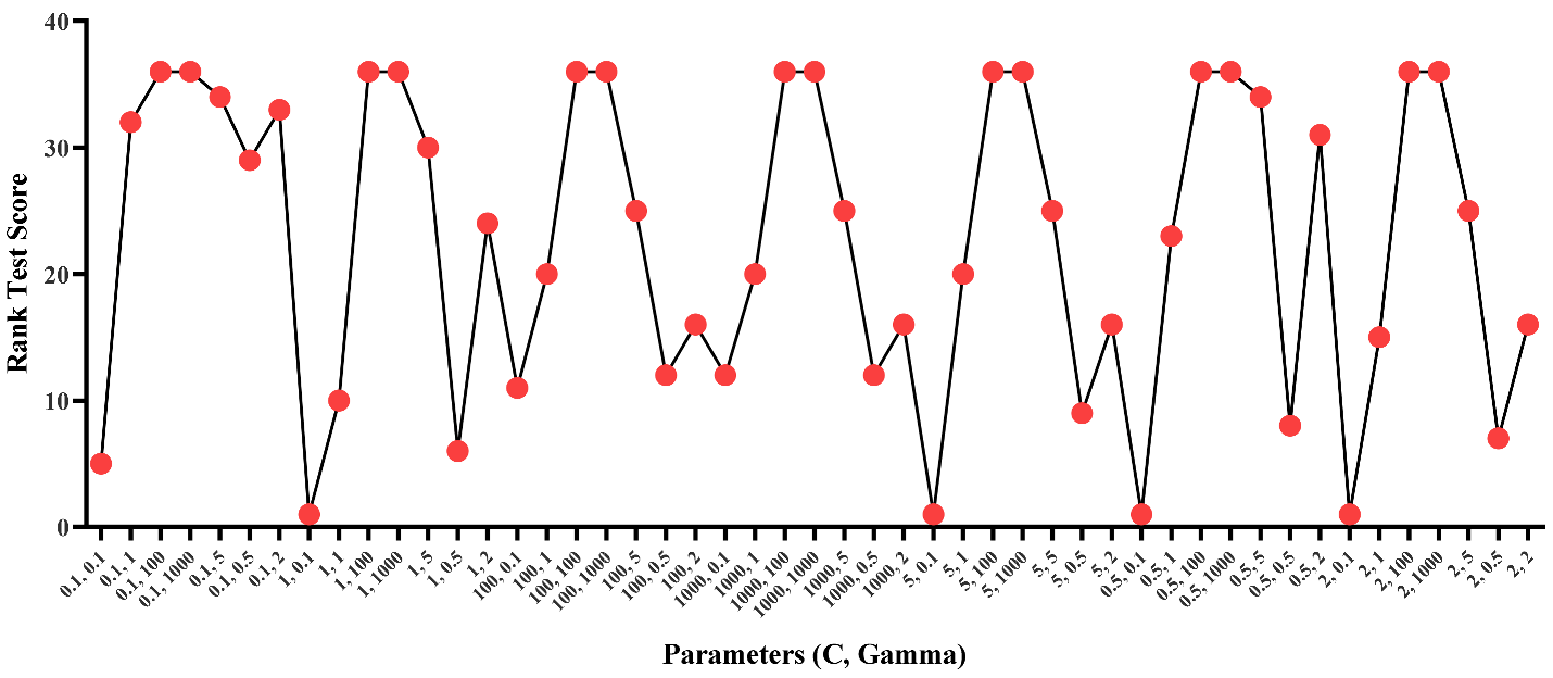
The study was implemented in Python 3.8.9. Sklearn library ver. 0.23.2 was used to implement ML models. Other libraries included NumPy ver. 1.18.5, Pandas ver. 1.3.3, matplotlib ver. 3.3.1 and Dalex ver. 1.4.1. The dataset was partitioned into training and testing using 70–30 distribution. A normalization technique was applied to SVM, since it is a linear-based model, to make it normally distributed in a standard scaler. Furthermore, a Recursive Feature Elimination (RFE) feature selection technique was applied while grid search and cross-validation were performed to find the best values for each algorithm parameter. 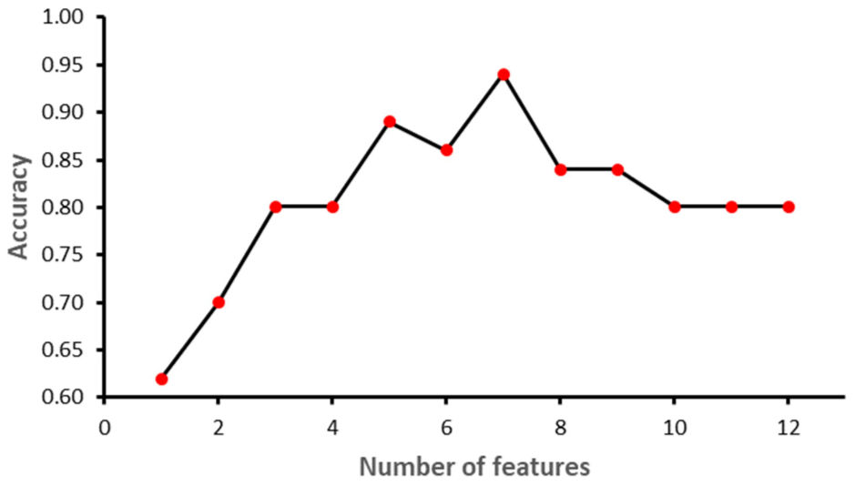Figure 6, Figure 7, Figure 8 and Figure 9 show the outcome of the RFE for each classifier. 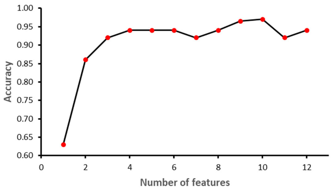Figure 6 shows that with seven features, while the SVM model achieved the highest performance in terms of accuracy. Initially, the performance of the model improved with the increase in the number of features, but with eight features the performance deteriorated. The selected features for SVM model were: ‘II’, ‘STV’, ‘LTI’, ‘MF_pow’, ‘HF_pow’, ‘LF/(MF + HF)’ and ‘ApEn(1, 0)’. However, for the RF model, the best performance was achieved with 10 features: ‘GA_CTG’, ‘DELTA’, ‘STV’, ‘LTI’, ‘LF_pow’, ‘HF_pow’, ‘LF/(MF + HF)’, ‘ApEn(1, 0.1)’, ‘LZC(2, 0)’ and ‘APRS’. 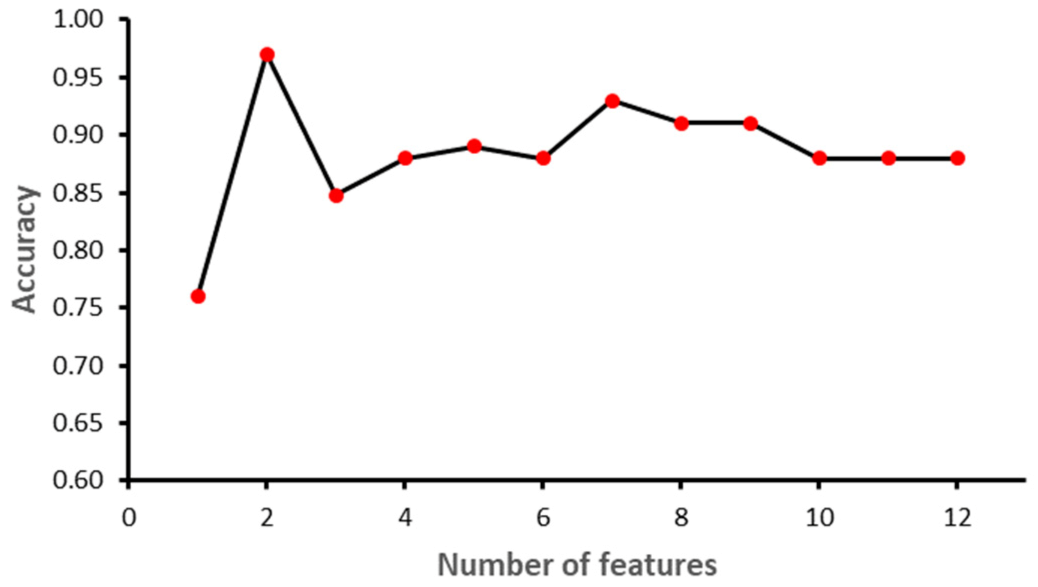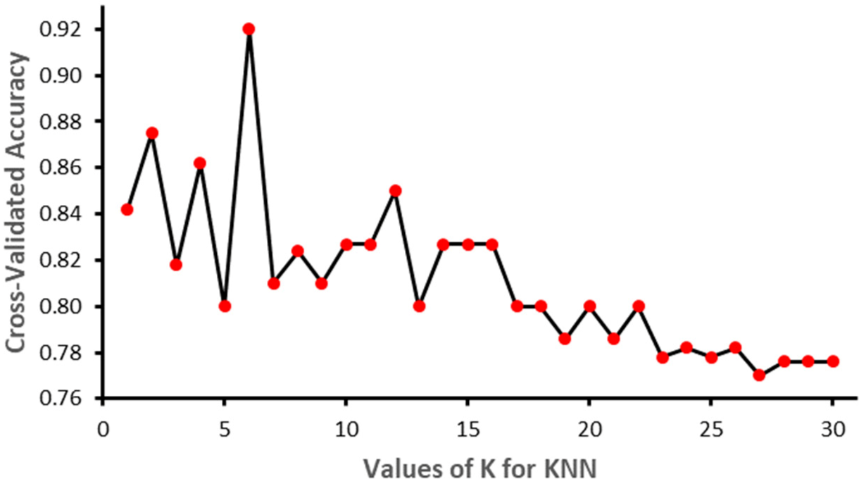Figure 7 shows the impact of feature selection on the performance of the RF model. The performance of the RF algorithm initially increased as the features were added, but after six features the performance degraded slightly; however, by eight features the performance start to increase again. 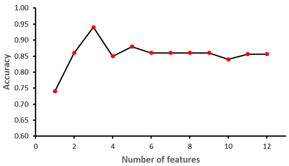Similarly, KNN achieved the best performance with two features, namely GA_CTG’ and ’LZC (2,0), as shown in the Figure 8. Finally, the GB model produced the best performance with three features: ‘GA_CTG’, ‘STV’ and ‘LTI’, as shown in Figure 9.

Table 6. Selected Features using Recursive Feature Elimination for each classifier.

Model	Selected Features
SVM	‘II’, ‘STV’, ‘LTI’, ‘MF_pow’, ‘HF_pow’, ‘LF/(MF + HF)’, ‘ApEn(1, 0)’
RF	‘GA_CTG’, ‘DELTA’, ‘STV’, ‘LTI’, ‘LF_pow’, ‘HF_pow’, ‘LF/(MF + HF)’, ‘ApEn(1, 0.1)’, ‘LZC(2, 0)’, ‘APRS’
KNN	GA_CTG’, ’LZC (2,0)
GB	‘GA_CTG’, ‘STV’, ‘LTI’

contains the selected features using RFE for each classifier.

The evaluation parameters used for comparing the classifiers’ performance in the study are Accuracy (ACC), Sensitivity (SN), Specificity (SP), Positive Predicted Value (PPV), Negative Predicted Value (PPV) and F1-score. The formula for the evaluation measures is represented in the equations below.

$$Accuracy \left(ACC\right) = \frac{sum of correctly predicted healthy fetus and IUGR fetus}{sum of all the samples used for the prediction}$$

$$Sensitivity \left(SN\right) = \frac{sum of correctly predicted IUGR fetus}{sum of all IUGR fetus samples used for the prediction}$$

$$Specificity \left(SP\right) = \frac{sum of correctly predicted Ihealthy fetus}{sum of all healthy fetus samples used for the prediction}$$

$$Positive Predictive Value \left(PPV\right) = \frac{sum of correctly predicted IUGR fetus}{sum of all the samples predicted as IUGR fetus}$$

$$Negative Predictive Value \left(PPV\right) = \frac{sum of correctly predicted healthy fetus}{sum of all the samples predicted as healthy fetus}$$

$$F1 = \frac{2\times \left(SN\times PPV\right)}{SN+PPV}$$

Table 7. Performance comparison of the models for antepartum fetus monitoring using dataset I.

Models	Feature Selection	No of features	ACC	SN	SP	F1	PPV	NPV
SVM	×	13	0.81	0.74	0.92	0.83	0.94	0.67
	√	7	0.94	0.9	1	0.95	1	0.89
RF	×	13	0.94	1	0.86	0.96	0.92	1
	√	10	0.97	1	0.92	0.98	0.96	1
KNN	×	13	0.81	1	0.63	0.83	0.71	1
	√	2	0.94	1	0.86	0.96	0.92	1
GB	×	13	0.86	0.95	0.73	0.89	0.83	0.92
	√	3	0.94	1	0.86	0.96	0.92	1

indicates the performance comparison of classifiers with and without feature selection technique using dataset I.

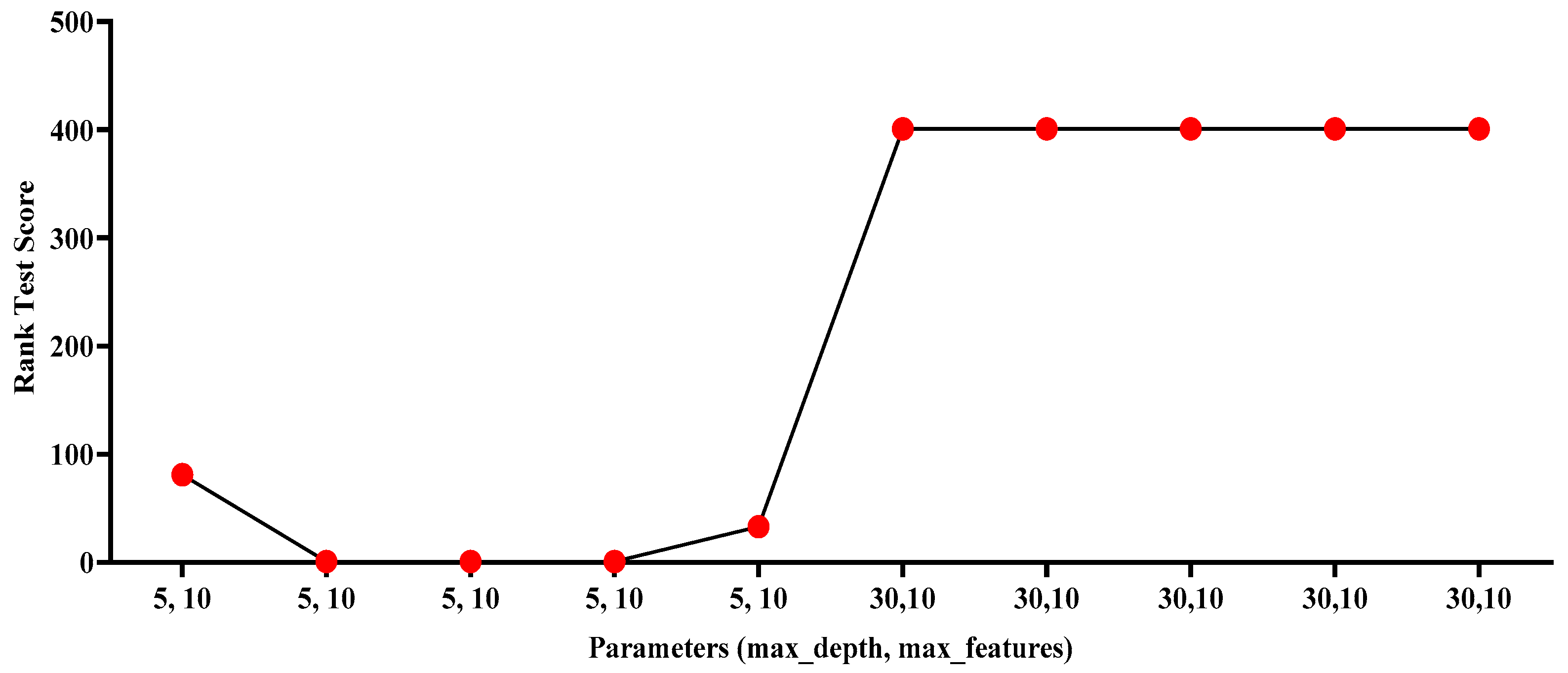
After applying feature selection with RFE, the accuracy increased to 0.92 in SVM, with n = 7 selected features; however, after optimizing the model with grid search by using the C and gamma parameters, the results increased to 0.94. In the case of RF, we applied feature selection with RFE and achieved the same with an accuracy of 0.94 with random state = 45 to have fixed accuracy results in each run and with n = 10 selected features. After that, the model was optimized with grid search by using the number of estimators, the maximum depth, the minimum samples split, the minimum samples leaf and the maximum features. The results increased to an accuracy of 0.97 with random state = 50 and n = 10 selected features. However, KNN model performance gives the same result with and without optimization. Due to the fact that KNN model is a lazy learner model and there are not huge parameters in the model. There was a minor increase in PPV and F1-score. However, the performance of the GB model was greatly improved after the optimization and feature selection. 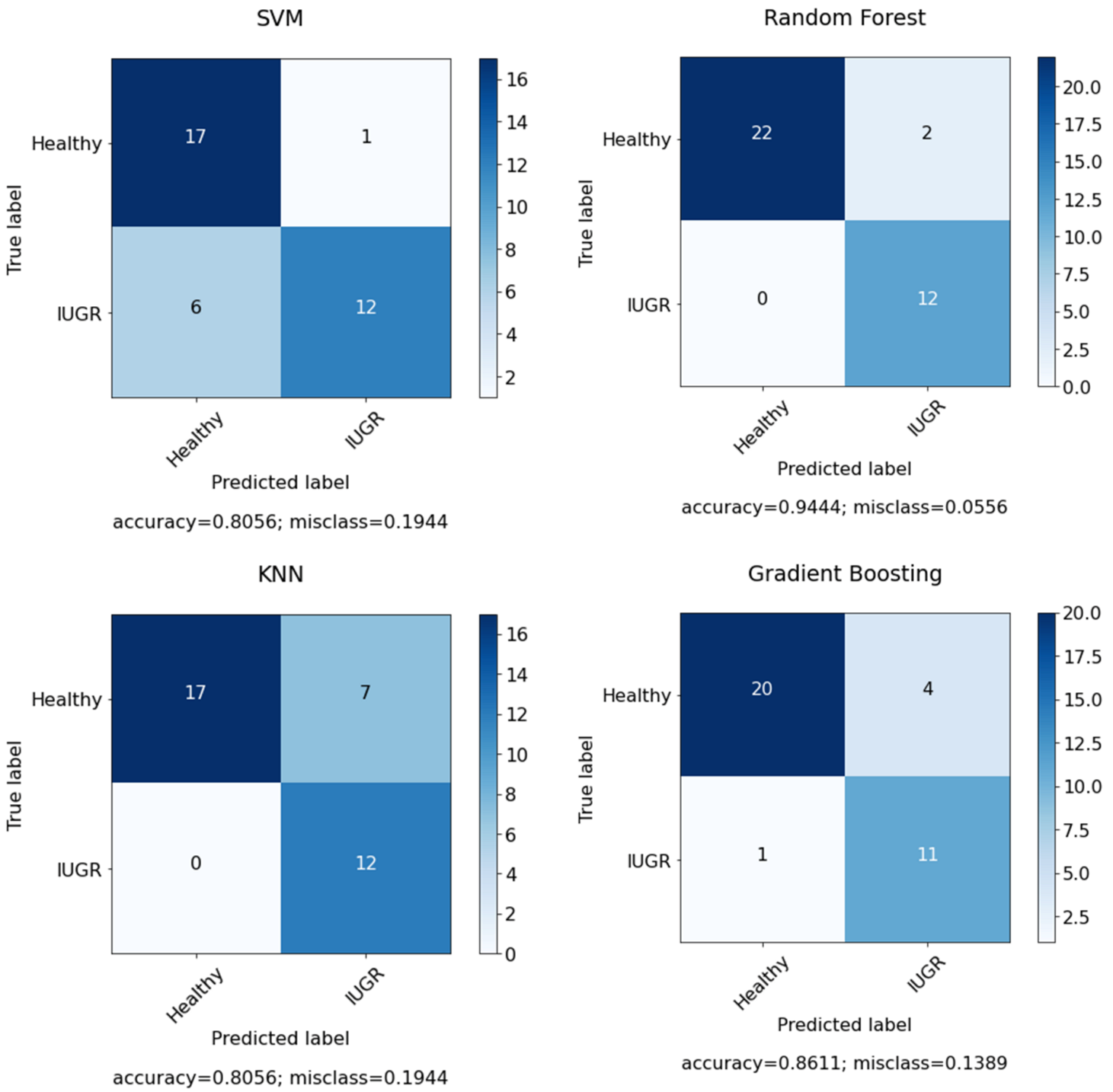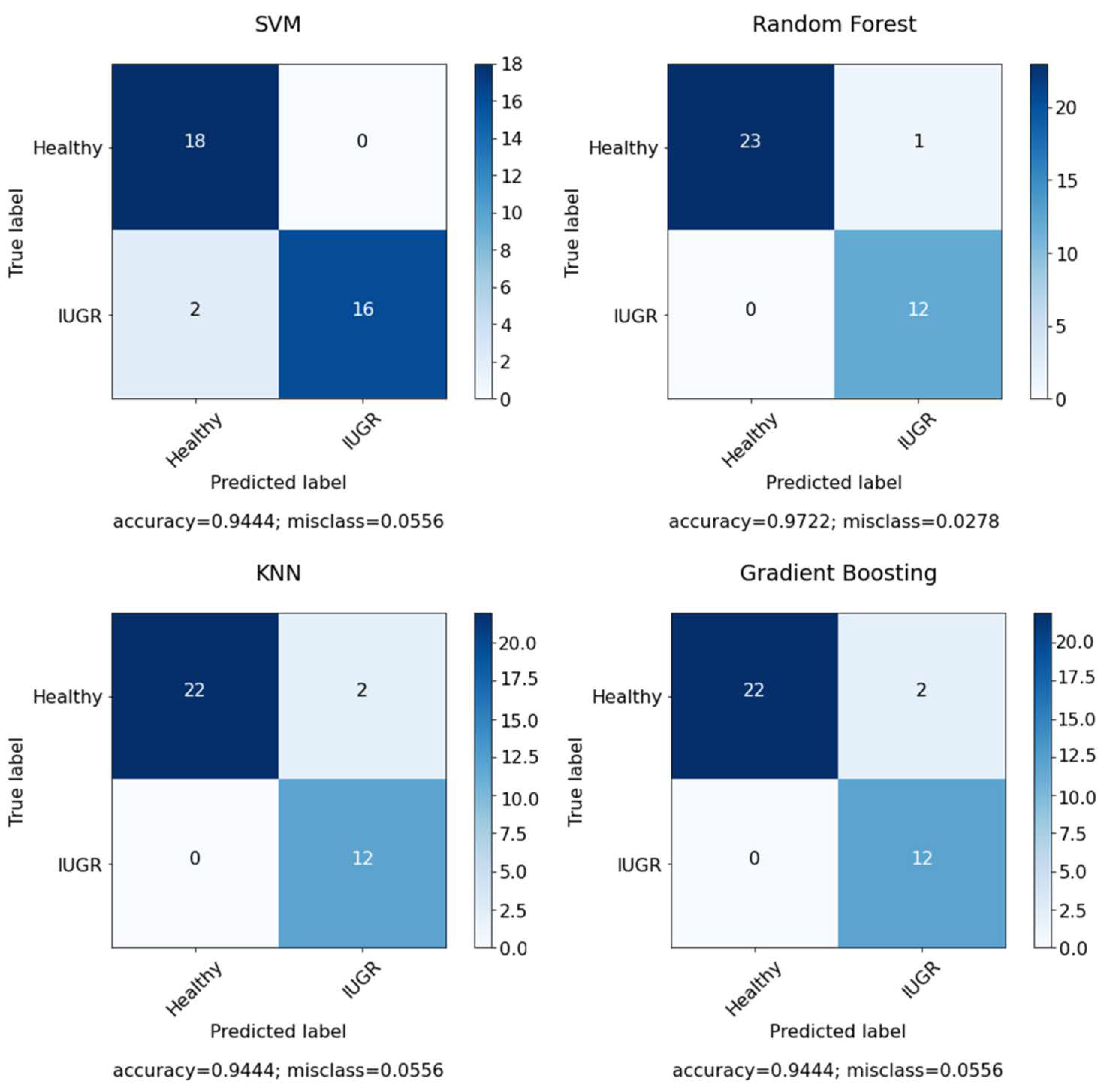Figure 10 presents the confusion matrix for the selected features using dataset I. However, Figure 11 shows the confusion matrix for the selected features and optimized models using dataset I.

The performance of the models was also compared with the baseline study. Initially, the performance of the model was compared with Signorini et al. [13], and later the best performing model was tested on Pini et al.’s [22] dataset using the selected features. Similar to baseline, RF outperformed the other models in terms of ACC, SN, PPV and NPV, while the SP value of the baseline study is similar to that of the proposed study. Furthermore, the number of features were also reduced, although Pini et al. [22] achieved the highest results with SVM by using the radial based kernel function. The proposed RF model has achieved better results in term of ACC, SP, PPV and NPV. However, the SN of the proposed model is slightly higher than that of Pini et al. [22].

Table 8. Comparison of the proposed model with the baseline study.

Study	Dataset	No of Features	Model	ACC	SN	SP	PPV	NPV
[13]	Dataset I	11	RF	0.911	0.902	0.919	0.936	0.918
Proposed Study		10	RF	0.97	1	0.92	0.96	1
[22]	Dataset II	10	SVM	0.84	0.843	0.85	0.9	0.77
Proposed		10	RF	0.87	0.85	0.92	0.96	0.73

presents the comparison of the proposed study and the baseline study.

Generating Explanation Using Explainable Artificial Intelligence (EAI)

Despite the significant outcome of the ML and DL models in the prediction, these techniques are also considered as a black box and lack interpretability and comprehensibility [30]. In the current study the explanation was generated using Shapley Additive Explanations (SHAP) and Local Interpretable Model-agnostic Explanations (LIME) to explain the prediction. SHAP uses game theory to generate the explanations to identify how each feature contributes to the prediction. Figure 12 shows the global mean importance mean (SHAP values). However, Figure 13 presents the information on one of the samples that is decomposed into attributes and the impact of each attribute, as well as the combined impact of the attributes for that particular sample. LIME is used to generate the explanation.

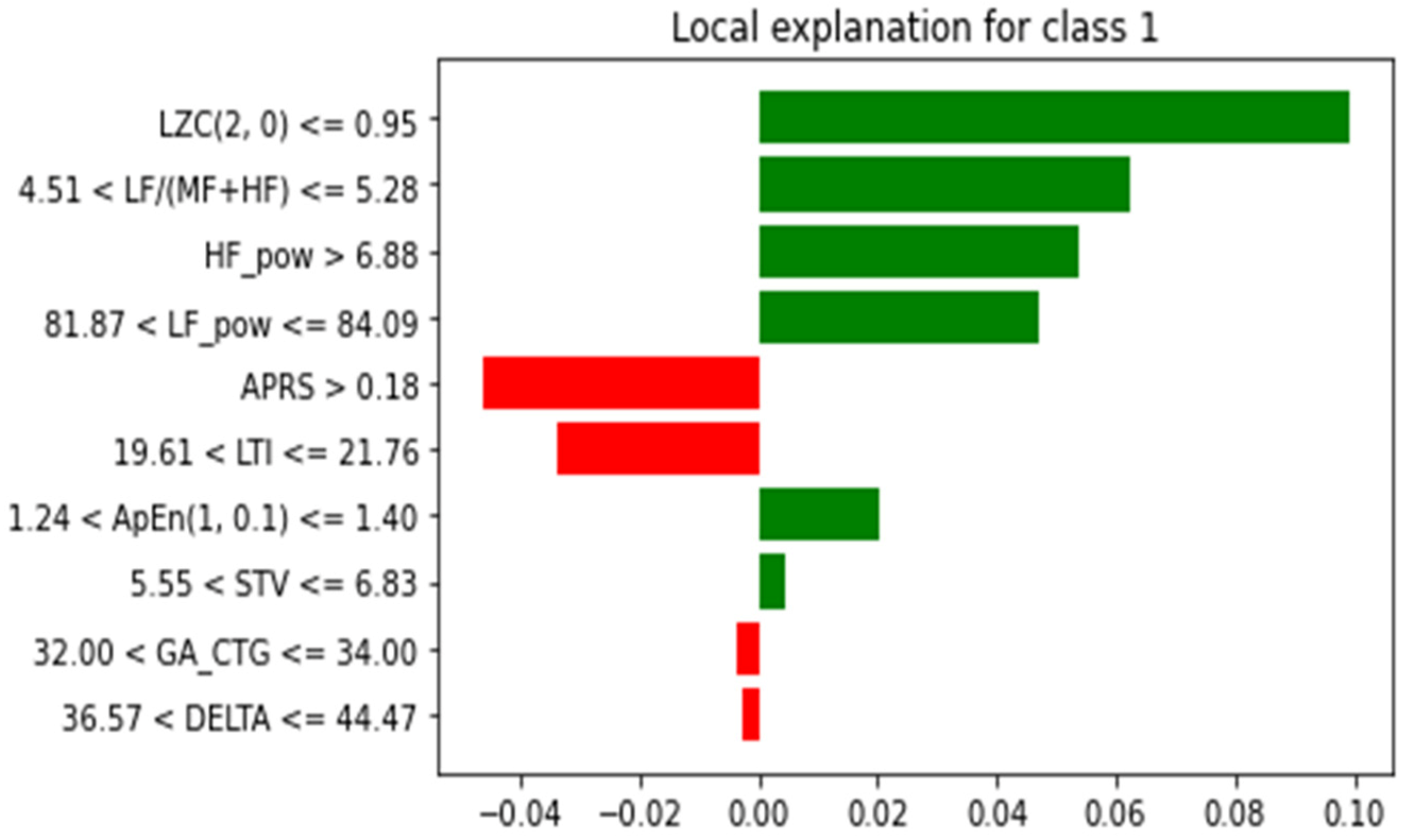
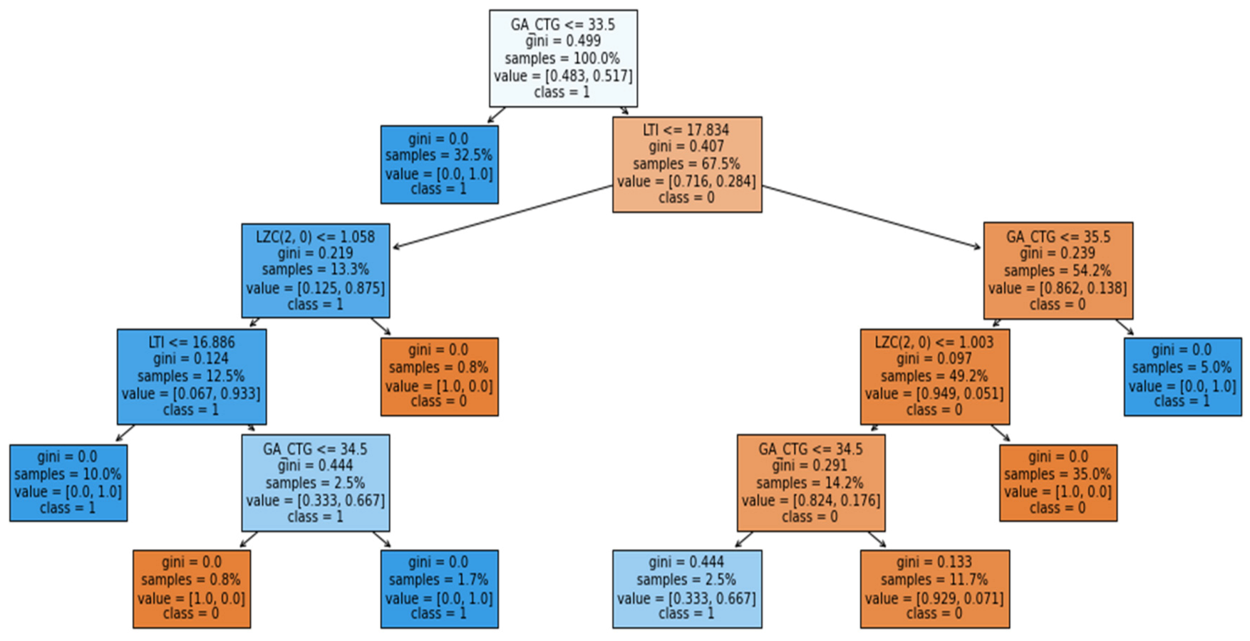
As can be seen from Figure 13, for predicting the IUGR represented as class 1, the green bar indicates that it supports the model that makes the prediction. In the figure, the name of the attribute is mentioned along with some value and range. This indicates that, during prediction, these specific values of the attributes help the model make the prediction (represented by the green bar). However, when represented by red, they indicate that the specific values of these attributes, such as APRS > 0.18, 81.87 < LF_pow <= 84.09, 32.00 < GA <= 34.00 and 36.57 < DELTA <= 44.47, not very well supported. However, this does not mean that these attributes are not significant; it only explains the prediction of that particular sample using the proposed RF model. In addition, for further interpretation the explanation of the RF model was generated in terms of the tree structure, as shown in Figure 14.

The main contribution of the study is:

• To introduce Explainable Artificial Intelligence (EAI) in fetus antepartum monitoring using FHR.
• To propose an enhanced model with improved performance and a reduced set of features.
• To further validate the model with another dataset. Indeed, the model outperformed the two baseline models.

In spite of all these advantages, there is one limitation and that is the size of the dataset.

5. Conclusions

Analysis of the FHR for Antepartum Fetal health monitoring to determine the Healthy/IUGR fetus is a standard technique used in clinical practice to maintain fetal health during pregnancy. The study used several machine learning algorithms, such as SVM, RF, KNN and GB. Feature selection was performed using RFE and optimization by using a grid search technique. The experiments were made using two datasets, and RF achieved the highest results in terms of all the measures. Furthermore, explanations were generated using LIME and SHAP, and the induced tree was employed to extract rules from the classifiers. It is worth mentioning that the proposed study outperformed the baselines in terms of all the performance measures using reduced number of features. Conclusively, the proposed model can assist the doctor in predicting the fetus as normal or IUGR and will help in providing the essential medical treatment at the proper time to maintain the fetus’ well-being. Notwithstanding these benefits, the proposed model needs to be further investigated via its huge dataset.

References

1. WHO. Preterm-Birth. Available online: http://www.who.int/en/news-room/fact-sheets/detail/preterm-birth (accessed on 26 May 2021).
2. Premature-Birth-Facts-and-Statistics. Available online: https://www.verywellfamily.com/premature-birth-facts-and-statistics-2748469 (accessed on 25 May 2021).
3. Committee on Practice Bulletins–Gynecology, American College of Obstetricians and Gynecologists. Intrauterine growth restriction: Clinical management guidelines for obstetrician-gynecologists. Int. J. Gynaecol. Obs. 2001, 72, 85–96. [Google Scholar] [CrossRef]
4. Gürgen, F.; Zengin, Z.; Varol, F. Intrauterine growth restriction (IUGR) risk decision based on support vector machines. Expert Syst. Appl. 2012, 39, 2872–2876. [Google Scholar] [CrossRef] [Green Version]
5. Corizzo, R.; Dauphin, Y.; Bellinger, C.; Zdravevski, E.; Japkowicz, N. Explainable image analysis for decision support in medical healthcare. In Proceedings of the 2021 IEEE International Conference on Big Data (Big Data), Orlando, FL, USA, 15–18 December 2021; pp. 4667–4674. [Google Scholar] [CrossRef]
6. Tonkovic, P.; Kalajdziski, S.; Zdravevski, E.; Lameski, P.; Trajkovik, V. Literature on applied machine learning in metagenomic classification: A scoping review. Biology 2020, 9, 453. [Google Scholar] [CrossRef] [PubMed]
7. Bote-Curiel, L.; Muñoz-Romero, S.; Gerrero-Curieses, A.; Rojo-Álvarez, J.L. Deep learning and big data in healthcare: A double review for critical beginners. Appl. Sci. 2019, 9, 2331. [Google Scholar] [CrossRef] [Green Version]
8. Ngiam, K.Y.; Khor, I.W. Big data and machine learning algorithms for health-care delivery. Lancet Oncol. 2019, 20, e262–e273. [Google Scholar] [CrossRef]
9. Sidey-Gibbons, J.A.M.; Sidey-Gibbons, C.J. Machine learning in medicine: A practical introduction. BMC Med. Res. Methodol. 2019, 19, 64. [Google Scholar] [CrossRef] [PubMed] [Green Version]
10. Oprescu, A.M.; Miró-Amarante, G.; García-Díaz, L.; Beltrán, L.M.; Rey, V.E.; Romero-Ternero, M. Artificial intelligence in pregnancy: A scoping review. IEEE Access 2020, 8, 181450–181484. [Google Scholar] [CrossRef]
11. Doran, D.; Schulz, S.; Besold, T.R. What does explainable AI really mean? A new conceptualization of perspectives. arXiv 2017, arXiv:1710.00794. [Google Scholar]
12. Lötsch, J.; Kringel, D.; Ultsch, A. Explainable artificial intelligence (XAI) in biomedicine: Making AI decisions trustworthy for physicians and patients. BioMedInformatics 2022, 2, 1–17. [Google Scholar] [CrossRef]
13. Signorini, M.G.; Pini, N.; Malovini, A.; Bellazzi, R.; Magenes, G. Integrating machine learning techniques and physiology based heart rate features for antepartum fetal monitoring. Comput. Methods Programs Biomed. 2020, 185, 105015. [Google Scholar] [CrossRef] [PubMed]
14. van Nguyen, S.; Lobo Marques, J.A.; Biala, T.A.; Li, Y. Identification of latent risk clinical attributes for children born under iugr condition using machine learning techniques. Comput. Methods Programs Biomed. 2020, 200, 105842. [Google Scholar] [CrossRef] [PubMed]
15. Zhao, Z.; Zhang, Y.; Deng, Y. A comprehensive feature analysis of the fetal heart rate signal for the intelligent assessment of fetal state. J. Clin. Med. 2018, 7, 223. [Google Scholar] [CrossRef] [PubMed] [Green Version]
16. Magenes, G.; Bellazzi, R.; Fanelli, A.; Signorini, M.G. Multivariate analysis based on linear and non-linear FHR parameters for the identification of IUGR fetuses. In Proceedings of the 2014 36th Annual International Conference of the IEEE Engineering in Medicine and Biology Society, Chicago, IL, USA, 26–30 August 2014; pp. 1868–1871. [Google Scholar] [CrossRef]
17. Cömert, Z.; Kocamaz, A.F. Comparison of machine learning techniques for fetal heart rate classification. Acta Phys. Pol. A 2017, 132, 451–454. [Google Scholar] [CrossRef]
18. Signorini, M.G.; Magenes, G. Reliable nonlinear indices for fetal heart rate variability signal analysis. In Proceedings of the 2014 8th Conference of the European Study Group on Cardiovascular Oscillations (ESGCO), Trento, Italy, 25–28 May 2014; pp. 213–214. [Google Scholar] [CrossRef]
19. Chaaban, R.; Issa, W.; Bouakaz, A.; Zaylaa, A.J. Hypertensive disorders of pregnancy: Kurtosis-based classification of fetal doppler ultrasound signals. In Proceedings of the 2019 Fifth International Conference on Advances in Biomedical Engineering (ICABME), Tripoli, Lebanon, 17–19 October 2019. [Google Scholar] [CrossRef] [Green Version]
20. Moreira, M.W.L.; Rodrigues, J.J.P.C.; Furtado, V.; Mavromoustakis, C.X.; Kumar, N.; Woungang, I. Fetal birth weight estimation in high-risk pregnancies through machine learning techniques. In Proceedings of the 2019 IEEE International Conference on Communications (ICC), Shanghai, China, 20–24 May 2019. [Google Scholar] [CrossRef]
21. Krupa, N.; Ali, M.; Zahedi, E.; Ahmed, S.; Hassan, F.M. Antepartum fetal heart rate feature extraction and classification using empirical mode decomposition and support vector machine. Biomed. Eng. Online 2011, 10, 6. [Google Scholar] [CrossRef] [PubMed] [Green Version]
22. Pini, N.; Lucchini, M.; Esposito, G.; Tagliaferri, S. A machine learning approach to monitor the emergence of late intrauterine growth restriction. Front. Artif. Intell. 2021, 4, 622616. [Google Scholar] [CrossRef] [PubMed]
23. Caly, H.; Rabiei, H.; Coste-Mazeau, P.; Hantz, S.; Alain, S.; Eyraud, J.; Chianea, T.; Caly, C.; Makowski, D.; Hadjikhani, N.; et al. Machine learning analysis of pregnancy data enables early identification of a subpopulation of newborns with ASD. Sci. Rep. 2021, 11, 6877. [Google Scholar] [CrossRef] [PubMed]
24. Benhamou, S. Artificial intelligence and the future of work. Rev. D’Econ. Ind. 2020, 169, 57–88. [Google Scholar] [CrossRef]
25. Signorini, M.G.; Pini, N.; Malovini, A.; Bellazzi, R.; Magenes, G. Dataset on linear and non-linear indices for discriminating healthy and IUGR fetuses. Data Brief 2020, 29, 105164. [Google Scholar] [CrossRef] [PubMed]
26. Cortes, C.; Vapnik, V. Support-vector networks. Mach. Learn. 1995, 20, 273–297. [Google Scholar] [CrossRef]
27. Zhang, C.; Ma, Y. (Eds.) Ensemble Machine Learning; Springer: New York, NY, USA, 2012. [Google Scholar]
28. Han, J.; Pei, J.; Kamber, M. Data Mining: Concepts and Techniques; Morgan Kaufmann Publishers: San Francisco, CA, USA, 2001. [Google Scholar]
29. Janek, T. Gradient Boosting in Automatic Machine Learning: Feature Selection and Hyperparameter Optimization. Ph.D. Thesis, Ludwig Maximilian University of Munich, Munich, Germany, 2019. [Google Scholar]
30. Linardatos, P.; Papastefanopoulos, V.; Kotsiantis, S. Explainable AI: A review of machine learning interpretability methods. Entropy 2021, 23, 18. [Google Scholar] [CrossRef] [PubMed]
Figure 1. Attribute’s correlation heatmap for dataset I.
Electronics 11 00593 g001
Figure 2. Selected attribute’s correlation heatmap for dataset II.
Electronics 11 00593 g002
Figure 3. SVM Rank Test Score with different values of C and Gamma.
Electronics 11 00593 g003
Figure 4. Rank Test Score—RF with optimization values.
Electronics 11 00593 g004
Figure 5. Different value of K and the accuracy of the algorithm.
Electronics 11 00593 g005
Figure 6. Recursive Feature Elimination for Support Vector Machine.
Electronics 11 00593 g006
Figure 7. Recursive Feature Elimination for Random Forest.
Electronics 11 00593 g007
Figure 8. Recursive Feature Elimination for K Nearest Neighbor.
Electronics 11 00593 g008
Figure 9. Recursive Feature Elimination for Gradient Boosting.
Electronics 11 00593 g009
Figure 10. Confusion matrix for classifiers using all features in the dataset.
Electronics 11 00593 g010
Figure 11. Confusion matrix for classifiers using selected features in the dataset.
Electronics 11 00593 g011
Figure 12. Global feature importance mean ([SHAP value]).
Electronics 11 00593 g012
Figure 13. LIME for explaining the prediction for individual sample.
Electronics 11 00593 g013
Figure 14. Induced Decision Tree representation for the IUGR prediction Dataset I.
Electronics 11 00593 g014