Evaporation Forecasting through Interpretable Data Analysis Techniques

Abstract

Climate change is increasing temperatures and causing periods of water scarcity in arid and semi-arid climates. The agricultural sector is one of the most affected by these changes, having to optimise scarce water resources. An important phenomenon within the water cycle is the evaporation from water reservoirs, which implies a considerable amount of water lost during warmer periods of the year. Indeed, evaporation rate forecasting can help farmers grow crops more sustainably by managing water resources more efficiently in the context of precision agriculture. In this work, we expose an interpretable machine learning approach, based on a multivariate decision tree, to forecast the evaporation rate on a daily basis using data from an Internet of Things (IoT) infrastructure, which is deployed on a real irrigated plot located in Murcia (southeastern Spain). The climate data collected feed the models that provide a forecast of evaporation and a summary of the parameters involved in this process. Finally, the results of the interpretable presented model are validated with the best literature models for evaporation rate prediction, i.e., Artificial Neural Networks, obtaining results very similar to those obtained for them, reaching up to $0.85R^2$ and $0.6MAE$. Therefore, in this work, a double objective is faced: to maintain the performance obtained by the models most frequently used in the problem while maintaining the interpretability of the knowledge captured in it, which allows better understanding the problem and carrying out appropriate actions.

1. Introduction

Access to water is a fundamental right of today’s societies. It is a vital resource for living beings but also for the economic performance, growth, and viability of many business sectors [1]. However, it is also a finite and shared resource, whose indiscriminate consumption, whether by individuals, companies, or economic sectors, can have dramatic consequences for the common good. Therefore, optimising the use of water resources is a determining factor for the social and economic stability of modern societies [2]. The application of new technologies in these sectors, such as agriculture, guides the revolution of a society with an active role to face the related water scarcity problems [3].

Irrigated agriculture accounts for 20% of total cultivated land and contributes 40% of the total food produced in the world [4]. Fortunately, the agricultural sector is increasingly applying new technologies that improve its services and processes to increase profits, reduce costs, and make the system more sustainable [5]. Precision agriculture promotes the deployments of new technologies such as IoT or Artificial Intelligence in the sector of agriculture. This discipline covers issues ranging from pest detection to water saving, frost risk management, harvesting, and climate control of greenhouses, among others. Water shortage concerns are growing exponentially in many places around the world but, particularly, in arid or semi-arid regions such as southeastern Spain. These regions are suffering high temperatures and a lack of precipitation that causes periods of drought.

This climate scenario also impacts on the water storage used in irrigation due to evaporation increases [6]. Evaporation is the main component within the hydrological cycle and plays an important role in the planning, operation, and management of available water resources for agriculture [7]. In particular, evaporation losses can represent a significant part of the amount of water stored in a reservoir in semi-arid and arid regions with low rainfall. That makes it essential to consider evaporation estimates in the design of water management systems [8]. The evaporation rate can be calculated using direct or indirect methods [9]. Direct methods measure evaporation by means of pan or Piche evaporimeters. These methods are valid and reliable, but they are difficult to maintain, as manual and daily measurements are necessary. In contrast, indirect methods use meteorological variables to estimate the evaporation rate, which are based on mathematical models such as Penman–Monteith and Priestley–Taylor [10]. However, both methods are not able to achieve acceptable results for estimating evaporation data [11,12] as the physical process of evaporation is a highly non-linear problem; hence, the methods to be applied must take this aspect into account.

Machine learning (ML) techniques are efficient tools for solving complex, dynamic, and non-linear problems; they are capable of predicting different parameters through the relationships between inputs and outputs without considering the internal mechanisms of the system [13]. ML has been particularly applied in the field of agriculture [14] for crop management [15], yield prediction [16], disease detection [17], weed detection [18], crop recognition [19], crop quality [20], water management [21], soil management [22], and livestock management [23]. Regarding the evaporation prediction through ML models, some works have been proposed but mainly using ML methods as black box, i.e., the internals. The internals of these models are hidden, and therefore, users cannot understand the interactions between features. This hinders the estimation of the importance of each feature in the model predictions [24]. However, simpler models such as decision trees (DTs) may offer less predictive accuracy, and, in some complex scenarios, they are even able to model the inherent complexity of the dataset, but they are much easier to interpret and allow understanding the interactions in the modelling process [25,26]. This is particularly important when the system is intended to model physical phenomena, such as evaporation that has socioeconomic implications. Indeed, users need to know not only the prediction of the target variable (e.g., evaporation) but also the causes of the phenomenon in order to take corrective measures.

In this paper, we present an interpretable model, based on multivariate DTs, for the daily evaporation forecasting. We also validate this model by using an artificial neural network (ANN) model. Both models have been trained, validated, and tested with data from an IoT infrastructure deployment in an irrigated agricultural plot located in a semi-arid area of the Region of Murcia (Spain) that measures different meteorological and irrigation events and provides a two-year dataset, covering two dry and hot summer periods. In addition, for these two periods, the evaporation in the field has been recorded manually on a daily basis. In what follows, the main research objectives of this manuscript are addressed:

• Saving water in evaporation scenarios: The main objective of this work is to design and deploy a hardware and software infrastructure that, based on the monitoring of different meteorological components in irrigated plots, can predict the evaporation rate in following days to take actions that reduce water loss.
• Using an accurate and interpretable model: To achieve the above objective, the use of a multivariate DT model is proposed and subsequently evaluated to provide daily predictions of the evaporation rate. A white box model has been chosen; i.e., the influence of the input variables on the evaporation prediction can be understood.
• Data characterization: A two-year dataset of data from a real irrigated agricultural plot has been generated. This dataset has been used to develop the exposed models and is made available for the reproducibility of the results presented here.
• Assessment with black box methods: In addition to the interpretable method, a black box method has been used, specifically ANN, that is the most commonly used for this type of problem in the literature. The aim is to validate the interpretable model results by means of the black box method results.

The rest of the paper is structured as follows. First of all, Section 2 shows related works and the background necessary to better understand the main contribution of this paper. Section 3 shows the in situ IoT infrastructure deployed on the irrigation plot, the dataset layout generated, and the ML models used, their configuration and measures to assess results. Finally, Section 4 shows the performance and the result discussion of the methods targeted before the conclusions and future work are provided in Section 5.

2. Background

Since the early 1990s, ML techniques have started to be used in a wide range of problems related to water resources management such as precipitation forecasting, rainfall-runoff modelling, groundwater modelling, water quality assessment, sediment load prediction, and evaporation modelling. However, evaporation is considered the most difficult hydrological component to estimate. Although there are many works studying and assessing evaporation forecast, there is not any method that has demonstrated strong performance in all cases. In addition, the use of a particular method depends on the data availability, quality, and the application objectives. In general, studies show that ANN-based models perform better than more traditional techniques because they capture the non-linear nature of the problem [27]. However, since the evaporation problem is complex, researchers continue to work on obtaining accurate and reliable predictive models, highlighting the importance of reducing the number of measures used to obtain simpler models.

If we make a non-exhaustive study, in recent years, the analysis of various methods of evaporation forecasting from data using ML techniques has been carried out. Most of the studies explore the capabilities of ML techniques in various climates because each climate has its own characteristics of non-stationarity and stochasticity [28]. In addition, most of the studies analysed which combinations of weather measures are most suitable for building the models and compare the results obtained by ML models with the ones obtained by various empirical methods. The results in all of them indicate that ML models perform better than empirical ones.

In [8], the authors analysed the use of several ML techniques such as ANN, Least Squares–Support Vector Regression (LS-SVR), Fuzzy Logic, and ANFIS techniques to forecast the evaporation in subtropical climates. The most suitable set of measures to carry out evaporation forecasting was previously analysed by Gamma test. The authors concluded that the predictions made by ML models improved the results of the traditional Hargreaves and Samani and the Stephens–Stewart methods. The best results were obtained by Fuzzy Logic and LS-SVR techniques, and the measures needed in the estimations were minimum and maximum temperature, minimum and maximum humidity, rainfall, and sunshine hours.

The authors of [12] used an RBNN and an SVM to predict the evaporation rate in Malaysia taking into account two different scenarios. In the first scenario, they used time-series historical data, considering time increments to examine different patterns of data input and output. The second scenario used the mean temperature together with the historical evaporation rate. The best results were obtained by the RBNN.

In [29], evaporation forecasting with RBNN, self-organising map neural network, and multiple linear regression was carried out in Pantnagar (India). First, they carried out a selection of the most suitable combination of measures for the models using a Gamma test; then, they calibrated and validated the models for these combinations, and the results obtained were compared with empirical models. The best results were obtained with six variables and RBNN.

In [30], the authors carried out evaporation forecasting using SVR and ANN, and a combination of them with wavelet transforms at stations in Iran and Turkey. At the Iran station, the best result was obtained by ANN with temperature and solar radiation measures. At the Turkish station, the best result was obtained by ANN with temperature, relative humidity, and solar radiation measures. The combination with wavelet transforms was not substantially positive in reducing the error in either model.

In [27], the estimation of daily evaporation was performed using a combined MLP and krill herd optimisation model. They were applied to two stations in northern Iran. The results were compared with the measured ones with MLP and SVM models. The results obtained showed that the combined model had lower error. The bio-inspired krill herd optimisation algorithm was used to find the optimal neural network parameters.

Wu et al. [31] explored the benefits of coupling an extreme learning machine model with two new meta-heuristic algorithms, i.e., the whale optimisation algorithm and flower pollination algorithm for monthly pan evaporation prediction. Mohamady et al. [32] developed several models for monthly pan evaporation prediction. Particularly, they use optimisation approaches to train the adaptive neuro-fuzzy interface system (ANFIS), multilayer perceptron (MLP) model, and radial basis neural network (RBNN) model.

Another paper that also used the multilayer neural network and SVM was presented in [7]. The authors presented a hybrid model with a multilayer neural network and the Firefly algorithm that was used to predict daily evaporation using meteorological data from two stations in northern Iran. The Firefly algorithm was used to obtain the parameters of the multilayer neural network. The proposed model was compared with an unoptimised multilayer network and the SVM technique, with the hybrid model obtaining the best result.

In [11], the authors used four ML models for evaporation forecasting in Iraq from data provided by two weather stations in different climatic zones. A comparison of the different models in terms of accuracy was carried out, and the most appropriate set of measures to carry out the prediction was analysed. The paper concluded that in countries where there was not an adequate maintenance of weather stations, evaporation prediction by ML models was very interesting. The best results were obtained using the model obtained by SVM. Regarding the most interesting weather measures in the models, in each studied station, the set was different.

In [28], the authors worked with data obtained from two stations in Malaysia and apply three ML models: Extreme Gradient Boosting, ElasticNet Linear Regression, and Long Short-Term Memory and compared them with the empirical Stephens–Stewart and Thornthwaite techniques. The models were run on different types of measures, and the best results were obtained with Long Short-Term Memory. All machine learning models improved the empirical models.

The authors of [33] presented a study of ML techniques using climatological variables in three stations located in the Golestan province (Iran). The techniques used had been the Gaussian process, the K-nearest neighbours, the Random Forest, and the SVM for regression. The Gaussian process technique obtained better results with fewer climatic variables.

The previous literature review shows ML techniques have better performance than empirical ones. In addition, ANNs are a good option for modelling the evaporation forecast by using climate variables. However, ANN models act as a black-box and do not allow interpreting and understanding the model. Thus, it is not possible to extract knowledge from the process or the model. It would be interesting to obtain results comparable to those obtained with ANN models but with techniques that generate highly interpretable models. In this paper, we present an evaporation study with a twofold objective: good accuracy and interpretability.

3. Materials and Methods

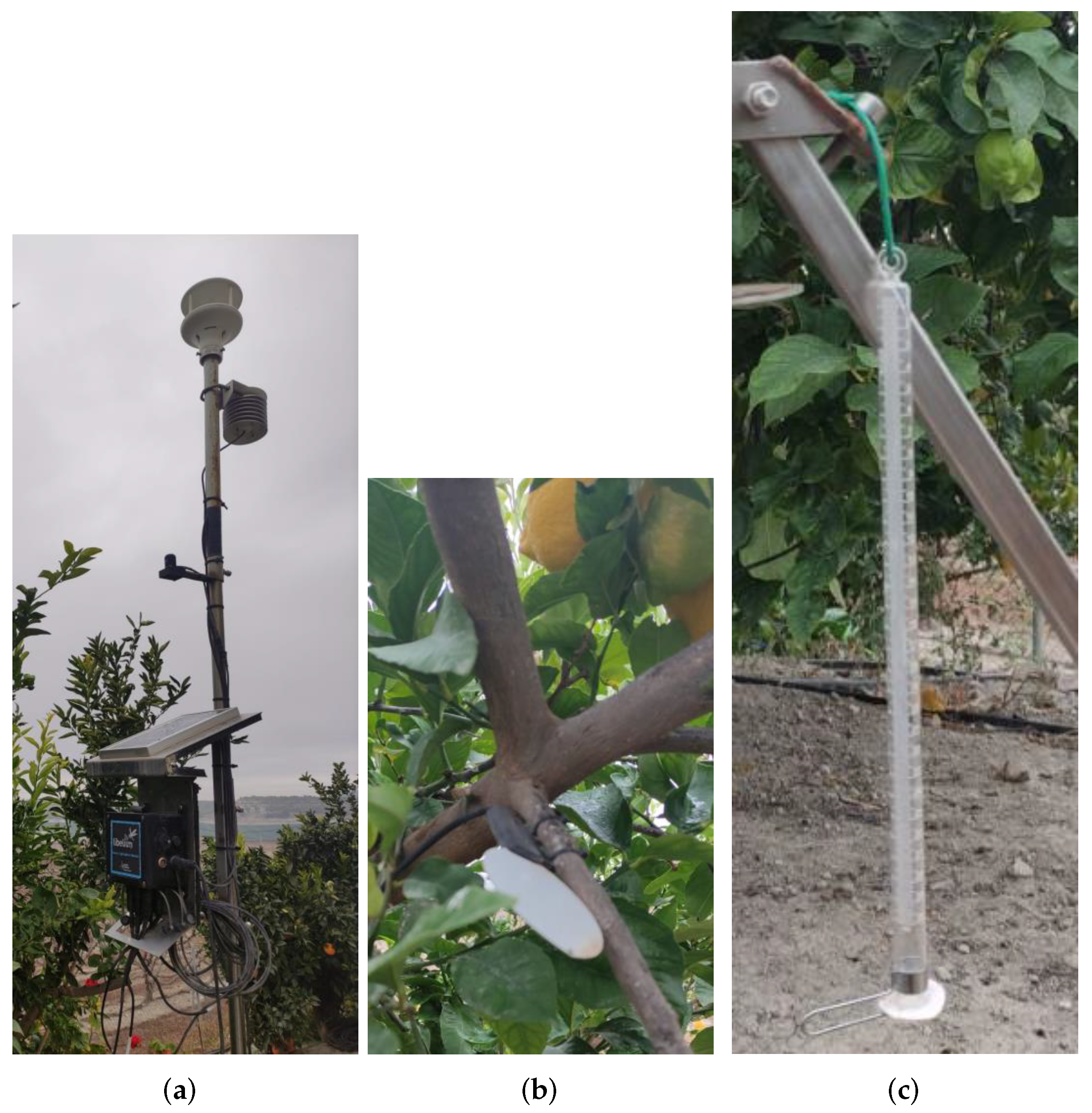
3.1. IoT Infrastructure

This study uses data from an IoT system deployed in a southeast Spain plot. The infrastructure was deployed and explained in [34]. The IoT system measures and saves periodical climate data. Libelium company (http://www.libelium.com/ (accessed on 23 December 2021)) provided and installed a Smart Agriculture Xtreme device in the plot. It enables the monitoring of multiple environmental parameters in a wide range of applications, from plant growth analysis to weather observation. Sensors are available for atmospheric, soil monitoring, and plant health. Figure 1 shows part of the IoT infrastructure and some sensors in detail. The sensors used in this study are as follows:

• Apogee SQ-100x: Collects photosynthetically active radiation expressed as photosynthetic photon flux density (photon flux in units of micromoles per square meter per second).
• Meter ATMOS 14: Measures air temperature in Celsius degrees, air humidity in percent, barometric pressure, and vapour pressure in kilo Pascals.
• Teros 12: Measures soil temperature in Celsius degrees, soil conductivity, and soil permeability in deciSiemens.
• MaxiMet GMX: Measures wind velocity in meters per second.

The IoT infrastructure has three main sub-modules with three sensors connected to each of them (i.e., humidity, temperature, and wind speed). Each sub-module communicates with the central module (actuator) using LoRa technology. LoRa enables long-distance communications, which allows the sensors to be dispersed in the agricultural field, keeping the connection to the local network. Finally, the module sends data to the cloud; specifically, the data are stored in an Amazon Web Services database. In addition to IoT infrastructure, we measure daily evaporation using a Piche evaporimeter; see Figure 1c. From it, we collected two seasons of data manually every day during the warmer and drier months in the region of Murcia.

3.2. Dataset

The IoT infrastructures and instrumentation described above have been used to generate a real dataset from an irrigated plot located in Cieza (Murcia, Spain). The dataset is structured as follows. Firstly, continuous meteorological data are available from the deployed Libelium IoT infrastructure since February 2020 at a 15-min granularity. As the objective of this paper focuses on the daily evaporation forecast, these data have been processed and grouped to generate the daily mean of these variables. Moreover, the dataset has been completed with the evaporation rate measured manually using the evaporimeter described above. In particular, it has been collected during the driest periods of the hydrological year in the study region. They started to be obtained from 3 August to 27 October 2020 and from 15 April to 5 September 2021.

Some authors include “Hydrometrical deficit or balance” (HD) as a variable to predict evaporation. The HD is calculated on the basis of certain climate variables, where the most common equation is $E=K\times HD$, where K sets out the relation with other climate variables such as wind velocity, air temperature, etc. [35]. In our case, we are going to include in the dataset the variable HD to study if it is relevant. However, the above equation is not going to be used, since in this work, the evaporation prediction is going to be done by other techniques. Thus, $HD$ is defined as the difference between the saturated vapour pressure at the free surface $Ea$ and at the ambient conditions $VP$.

$$HD=(Ea-VP)$$

(1)

Unfortunately, the in situ infrastructure described above does not provide $Ea$ as such. However, it is known that Relative Humidity ($RH$) can be obtained from $RH=\frac{VP}{Ea}\times 100$, from which $Ea=\frac{VP}{RH}\times 100$.

Replacing this value $Ea$ in Equation (1), $HD$ can be rewritten as $HD=\frac{VP\times 100}{RH}-VP$, which allows us to obtain $HD$ from the measurements provided by our infrastructure.

Summing up, the dataset under study brings together these meteorological and evaporation data, which includes 216 total observations. The dataset includes the following variables: “Soil Temperature” ($ST$), “Soil Permeability” ($SP$), “Soil Conductivity” ($SC$), “Air Temperature” ($AT$), “Wind Velocity” ($WV$), “Vapour Pressure” ($VP$), “Relative Humidity” ($RH$), “Air Pressure” ($AP$), “Solar Radiance” ($SR$), “Hydrometrical deficit” ($HD$), and the output variable “Evaporation” (E). The measurement units for the different climatic variables are °C, dS/s, dS/s, °C, m/s, kPa, %, kPa, μmol/m²/s, kPa, and mm, respectively. Therefore, each instance is described by the values of 10 climate variables and 1 output variable.

3.3. Techniques Used, Their Configuration, and Measures to Assess Results

This section briefly describes the techniques used for the regression process: an Artificial Neural Network and a Decision Tree. Although one of the more popular techniques to solve the regression task is the conventional regression analysis method, due to the rise of ANN and DT techniques, researchers are starting to use them, obtaining good results [36]. In addition, the configurations used in the experiments are detailed, and the different measures used to asses results are indicated.

3.3.1. Artificial Neural Network Technique

ANN models are one of the most widely used ML models. They imitate the way that biological neurons learn. The most common learning algorithm for this classifier is known as backpropagation. In the training phase, it adjusts the values of the weights of its neurons so that an input pattern generates a target output [37,38].

One of ANN’s difficulties is to choose a correct architecture, i.e., the number of hidden layers, neurons per layer, learning rate, etc. For this purpose, the optimal architecture has been defined by testing different values of its hyperparameters: among them, the $relu$ and $tanh$ activation functions have been tested, being the functions that activate neurons within the ANN; constant and adaptive learning rate, it is the rate schedule for weight updates; the solver function that optimises weights, such as $sgd$ and $adam$; internal validation percentages of $10\%$ and $20\%$ [39]; with or without early stopping, to terminate training when the validation score does not improve; and different values for maximum iterations, penalty parameter alpha, and the number of hidden neurons has been tested. The ANN architecture and hyperparameters configuration used in this work will be given in Section 4. All parameters and hyperparameters have been optimised by performing a set of additional tests to get the most optimal ones for the given problem.

In addition, the Python library sklearn has been used to create the ANN, where the model used is the MLPRegressor [40].

3.3.2. Decision Tree Technique

A DT is a tree structure in which each internal node corresponds to a question about one of the variables and each leaf node corresponds to a prediction for the output variable. A DT can be seen as a rules set of the form “if x then y”, where each rule is a branch from the root node to each leaf node of the DT. The DT model-base techniques allow both classification and regression tasks to be performed [41]. The DTs for the regression task obtain numerical values at the leaf nodes. The M5P technique obtains DTs for regression [42]. This technique builds regression trees with the characteristic that the leaf nodes contain multivariate regression models, which are used to obtain the numerical values as predictions [43]. Specifically, the M5P technique obtains leaf nodes of the form $w_1\times att{r}_1+\dots +w_n\times att{r}_n+w$, and therefore, the rules (branches of the regression tree) show relationships of the form:

if ($att{r}_1=v_1$) and … and ($att{r}_p=v_p$) then $Y=w_1\times att{r}_1+\dots +w_n\times att{r}_n+w$.

The M5P technique has been run using Weka workbench [44]. The stop condition in the construction of a branch of the regression tree is “number of instances M in the node”. The values of the parameter M that obtain the different results will be given in Section 4.

3.3.3. Measures Used to Assess Results, Validating Experiments

For all experiments, 5-fold cross-validation averaged 3 times (denoted 3 × 5 cv) is performed. That is, the dataset is divided into 5 equal parts, and 5 different models are obtained by taking 4 parts to learn the model and the remaining part as a test. This process is repeated 3 times. The measure used to evaluate shows the average value of the 15 models obtained [45]. In addition, an evaluation with a complete training dataset is carried out. Given the real data for variable X (evaporation) and their predictions Y (obtained by the corresponding techniques), different measures [46] are used to evaluate the predictions quality. These measures are defined as follows:

• Coefficient of determination ($R^2$) between two samples, observed values X and predictor values Y, measures the proportion of the variance in the sample X that is predictable from the sample Y. It is defined as $R^2(X,Y)=1-\frac{{\sum }_{i=1}^n{(x_i-y_i)}^2}{{\sum }_{i=1}^n{(x_i-\overline{X})}^2}\in [0,1]$ where $\overline{X}$ is the mean of the sample. High values of the measure indicate a behaviour highly reliable for future forecast of X by Y.
• Pearson Correlation Coefficient ($CC$) between two samples, X and Y, measures the linear statistical correlation between X and its prediction Y. This measure is defined as $CC(X,Y)=\frac{Cov(X,Y)}{{\sigma }_X{\sigma }_y}\in [-1,1]$ where $Cov$ is the covariance between X and Y, and ${\sigma }_X$ and ${\sigma }_Y$ are the standard deviation of X and Y, respectively. If $CC(X,Y)\in [0.5,1]$, there is a strong positive correlation (when X is increased, there is also an increase in Y) and if $CC(X,Y)\in [-1,-0.5]$, there is a strong negative correlation (there is a inverse relation between X and Y, when X is increased, Y is decreased).
• Mean absolute error ($MAE$) between samples of observed values X and predictor values Y is defined as $MAE(X,Y)=\frac{1}{n}{\sum }_{i=1}^n|x_i-y_i|$.
• Mean squared error ($MSE$) between samples of observed values X and predictor values Y is defined as $MSE(X,Y)=\frac{1}{n}{\sum }_{i=1}^n{(x_i-y_i)}^2$.

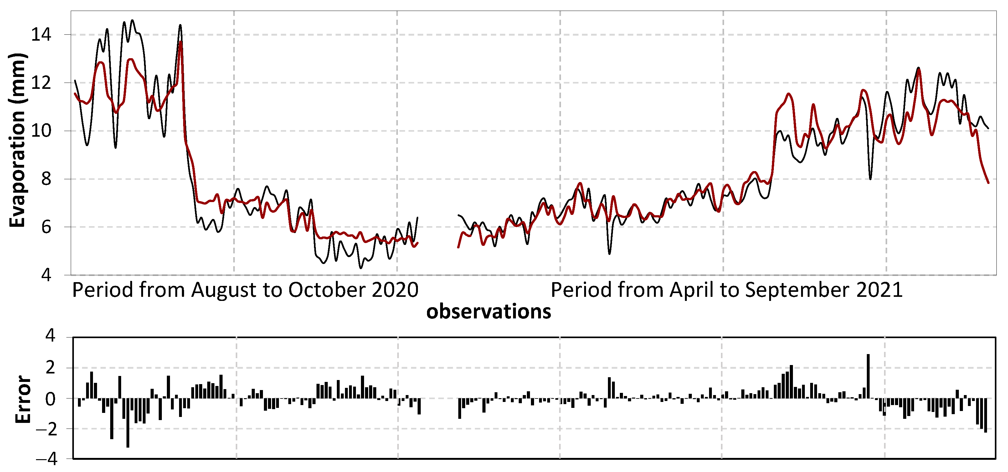
4. Results and Discussion

4.1. Preliminary Analysis

Table 1. Variable descriptive statistics. Mean, standard deviation (std), minimum (Min) and maximum (Max), and correlation with the measured evaporation (CC).

Variable		Mean	std	Min	Max	CC
Evaporation (E)		8.18	2.51	4.30	14.60	—
Soil Temperature ($ST$)		22.54	3.69	13.61	27.80	0.7814
Soil Permeability ($SP$)		8.40	0.96	7.04	13.25	−0.0974
Soil Conductivity ($SC$)		0.02	0.03	0.00	0.16	−0.2126
Air Temperature ($AT$)		29.18	5.25	12.20	40.60	0.7369
Wind Velocity ($WV$)		1.57	0.50	0.57	3.66	0.1711
Vapour Pressure ($VP$)		1.53	0.40	0.63	2.59	0.4835
Relative Humidity($RH$)		58.20	12.68	23.03	88.28	−0.3032
Air Pressure ($AP$)		97.68	0.36	96.23	98.46	−0.2648
Solar Radiance ($SR$)		484.85	156.72	10.94	949.18	0.2314
Hydrometrical deficit ($HD$)		1.16	0.53	0.16	2.72	0.6541

shows a descriptive analysis (mean, standard deviation, minimum and maximum) for all variables included in the dataset. Moreover, the linear correlation coefficient of each variable in the dataset with the manually measured evaporation is included.

Table 1 also describes how the variables with the highest correlation with respect to evaporation are soil temperature and air temperature followed by hydrometrical balance and vapour pressure. Weakly and inversely correlated with evaporation are the variables, in decreasing order, solar radiation, wind velocity, soil permeability, soil conductivity, air pressure, and relative humidity.

4.2. Black Box and Interpretable Models

Next, by applying the ANN and DT techniques presented, the relationship between all the input variables and the evaporation output is studied. To do that, two tests are performed using different dataset variables. The two dataset configurations, denoted $datase{t}_1$ and $datase{t}_2$, differ in different variables derived from the use or not of the variable $HD$ (these datasets are available on the website http://www.vielca.com/web/pages/proyectos/idi/gestion_recursos_waterot.php (accessed on 23 December 2021)).

• $datase{t}_1$: Obtained from nine variables (all variables of the dataset except the variable $HD$) to predict the output variable E.
• $datase{t}_2$: Obtained from eight variables (all variables of the dataset except the variables $VP$ and $RH$) to predict the output variable E.

The models obtained with the different dataset configurations are denoted by (Model A)${}_t$ and (Model B)${}_t$ indicating with the subscript t the technique (ANN or DT) used.

4.2.1. Artificial Neural Networks for Regression

Table 2. Artificial Neural Network hyperparameters.

Parameter	Value	Parameter	Value
$hidden\_layer\_sizes$	(120, 80, 40)	$learning\_rateinit$	0.01
$activation$	relu	$alpha$	0.0001
$solver$	adam	$early\_stopping$	True
$learning\_rate$	adaptive	$validation\_fraction$	0.2
$max\_iter$	3000

shows the best optimised parameters for (models A)${}_{ANN}$ and (model B)${}_{ANN}$.

Table 3. Artificial Neural Network results. Values (mean and standard deviation) of the different measures when using a 3 × 5-fold cross-validation and when using the whole dataset as training are shown.

	${\left(\mathbf{Model}\mathbf{A}\right)}_{\mathit{ANN}}$		${\left(\mathbf{Model}\mathbf{B}\right)}_{\mathit{ANN}}$
	$3\times 5\mathbf{cv}$	Training	$3\times 5\mathbf{cv}$	Training
$R^2$	$0.8265$ ($0.0128$)	$0.8842$	$0.8287$ ($0.0156$)	$0.8870$
$CC$	$0.9091$ ($0.0070$)	$0.9405$	$0.9103$ ($0.0086$)	$0.9419$
$MAE$	$0.5800$ ($0.1030$)	$0.6286$	$0.6170$ ($0.0876$)	$0.6152$
$MSE$	$1.0391$ ($0.1089$)	$0.7289$	$1.2030$ ($0.0554$)	$0.7115$

shows the results for models A and B obtained by the ANN. It is noteworthy that at the $R^2$ level, both models are equivalent, but at the level of the MAE and MSE metric, model A obtains lower error.

4.2.2. Decision Tree for Regression

In the DT M5P, the best optimised parameters of M are 16 and 23 for $datase{t}_1$ and $datase{t}_2$, respectively.

Table 4. Decision Tree results. Values (mean and standard deviation) of the different measures when using a 3 × 5-fold cross-validation and when using the whole dataset as training are shown.

	${\left(\mathbf{Model}\mathbf{A}\right)}_{\mathit{DT}}$		${\left(\mathbf{Model}\mathbf{B}\right)}_{\mathit{DT}}$
	$3\times 5\mathbf{cv}$	Training	$3\times 5\mathbf{cv}$	Training
$R^2$	$0.8448$ ($0.0056$)	$0.9004$	$0.8391$ ($0.0111$)	$0.8670$
$CC$	$0.9198$ ($0.0034$)	$0.9503$	$0.9162$ ($0.0062$)	$0.9390$
$MAE$	$0.7033$ ($0.0059$)	$0.5737$	$0.7449$ ($0.0451$)	$0.6217$
$MSE$	$0.9767$ ($0.0353$)	$0.6268$	$1.0128$ ($0.0701$)	$0.7529$

presents the results obtained by the DT M5P. The model that obtains better values (higher values for $R^2$ and $CC$, and lower values for $MAE$ and $MSE$ with smaller standard deviations) is the one that uses all variables except the variable $HD$ (model A)${}_{DT}$.

4.3. Analysis and Discussion

The results obtained by the ANN are satisfactory, and the models are robust and consistent, as indicated in the literature. However, ANN models are black box models, and it is not possible to draw a conclusion about which variables are the most significant or important. Thus, DT are proposed to improve the model’s interpretability. The results of the ANN and the DT are at the same level of accuracy, robustness, and satisfiability, and both models can be used as a predictive level. However, regarding the interpretability, the best model is the DT. Analysing the accuracy and fit of the two DT models, the best model is (model A)${}_{DT}$. This model is shown in Figure 2.

For illustrative purposes, Figure 3 shows the behaviour of (Model A)${}_{DT}$ in predicting the output variable E for the two used time periods. At the bottom of the figure is the residual error graph, showing for each observation the difference between the predicted value and the true value. As can be seen, the errors are minimal, and the obtained prediction is quite satisfactory.

Analysing the results in detail, (Model A)${}_{DT}$ obtains very satisfactory results: high value of the coefficient of determination ($R^2$) and an average error of 0.6 mm in the evaporation rate. The detailed analysis of the interpretable model (Model A)${}_{DT}$ is as follows:

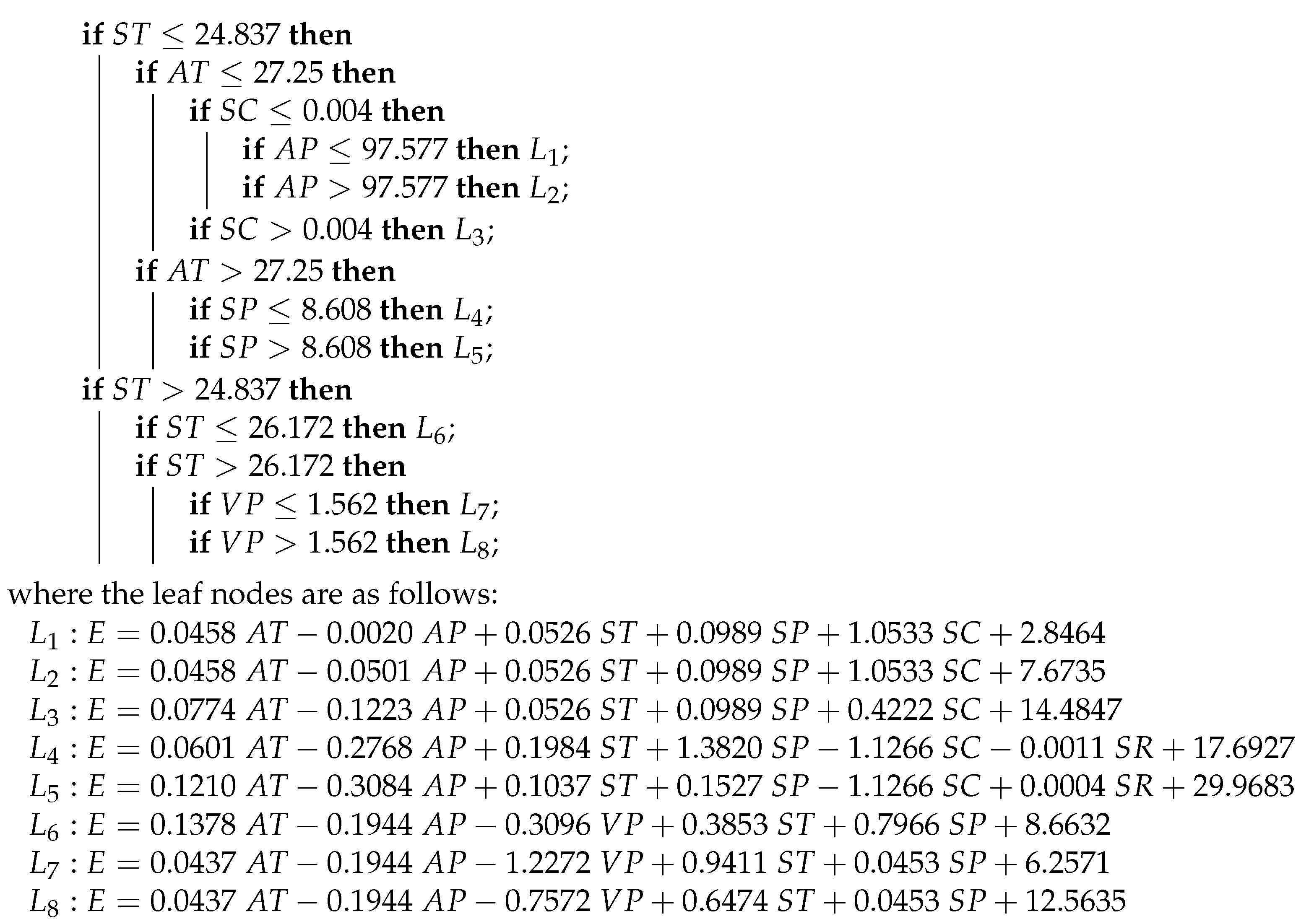
• The climate variables used in the model are Soil Temperature, Soil Permeability, Soil Conductivity, Air Temperature, Vapour Pressure, Air Pressure, and Solar Radiance.
• The climate variables that the model does not use are Relative Humidity and Wind Velocity. Therefore, these measures do not need to be collected.
• The discriminant climate variables are: Soil Temperature, Air Temperature, Soil Conductivity, Air Pressure, Soil Permeability, and Vapour Pressure.
• The most important climate variable is Soil Temperature.
• At a second level of importance, the climatic variables are Air Temperature and Vapour Pressure.
• If Soil Temperature is greater than 24.837 °C, then 37% of the predictions only use that variable with the support of the variable Vapour Pressure.
• If Soil Temperature is smaller than 24.837 °C, then 63% of the predictions are made with the support of the variables Air Temperature, Soil Conductivity, Air Pressure, and Soil Permeability.

  -

  If Air Temperature is smaller than 27.25 °C, then 32% of the predictions are made with the support of the variables Soil Conductivity and Air Pressure.

  -

  If Air Temperature is greater than 27.25 °C, then 31% of predictions are made with the support of the variable Soil Permeability.

With the detail of the model, the thresholds for each input variable describing the prediction of the evaporation rate can be checked. In addition to these thresholds, the most relevant variables and those that the model does not use are also specified. This can be understood by any non-technical person and can help to design a new IoT infrastructure with fewer sensors, thus reducing the economic cost of the infrastructure.

5. Conclusions and Future Work

Evaporation is one of the major reasons for water loss in irrigated agriculture. Mechanisms are in place to prevent evaporation losses in storage reservoirs to make the best use of this scarce resource. The problem with the evaporation rate is that it is a measure that has to be estimated or collected manually in order to be analysed. Then, this work presents an interpretable ML model to predict evaporation in irrigated agricultural plots on a daily basis. It is based on a multivariate DT for regression that takes information from an IoT system deployed in a real irrigated plot. The interpretable model achieves results with an average error of 0.6 mm in evaporation rate and a value of $R^2$ of 0.85. The exposed model obtains similar quality results to the ANN, (i.e., black box model) that has shown good results in the literature. However, this model also offers the possibility to understand which meteorological variables are most likely to affect the predicted evaporation. Thus, the climatic variables in the best DT model are Soil Temperature, Soil Permeability, Soil Conductivity, Air Temperature, Vapour Pressure, Air Pressure, and Solar Radiance. On the other hand, the variables Relative Humidity and Wind Velocity are not used, so in the future, they might not be necessary in a new IoT infrastructure. In addition, the proposed model as the best predictor allows that the farmer can cultivate in a sustainable way, realising better water management for irrigation. In fact, because evaporation prediction can affect irrigation decisions, in the future, we will work on obtaining sub-daily predictions to develop more efficient irrigation systems.

References

1. Garrick, D.E.; Hanemann, M.; Hepburn, C. Rethinking the economics of water: An assessment. Oxf. Rev. Econ. Policy 2020, 36, 1–23. [Google Scholar] [CrossRef] [Green Version]
2. Pahl-Wostl, C. An evolutionary perspective on water governance: From understanding to transformation. Water Resour. Manag. 2017, 31, 2917–2932. [Google Scholar] [CrossRef]
3. Kamienski, C.; Soininen, J.P.; Taumberger, M.; Dantas, R.; Toscano, A.; Salmon Cinotti, T.; Filev Maia, R.; Torre Neto, A. Smart water management platform: IoT-based precision irrigation for agriculture. Sensors 2019, 19, 276. [Google Scholar] [CrossRef] [PubMed] [Green Version]
4. Meier, J.; Zabel, F.; Mauser, W. A global approach to estimate irrigated areas–a comparison between different data and statistics. Hydrol. Earth Syst. Sci. 2018, 22, 1119–1133. [Google Scholar] [CrossRef] [Green Version]
5. Zhang, P.; Guo, Z.; Ullah, S.; Melagraki, G.; Afantitis, A.; Lynch, I. Nanotechnology and artificial intelligence to enable sustainable and precision agriculture. Nat. Plants 2021, 7, 864–876. [Google Scholar] [CrossRef]
6. Melgarejo-Moreno, J.; López-Ortiz, M.I.; Fernández-Aracil, P. Water distribution management in South-East Spain: A guaranteed system in a context of scarce resources. Sci. Total Environ. 2019, 648, 1384–1393. [Google Scholar] [CrossRef] [PubMed] [Green Version]
7. Ghorbani, M.; Deo, R.C.; Yaseen, Z.M.; Kashani, M.H.; Mohammadi, B. Pan evaporation prediction using a hybrid multilayer perceptron-firefly algorithm (MLP-FFA) model: Case study in North Iran. Theor. Appl. Climatol. 2018, 133, 1119–1131. [Google Scholar] [CrossRef]
8. Goyal, M.K.; Bharti, B.; Quilty, J.; Adamowski, J.; Pandey, A. Modeling of daily pan evaporation in sub tropical climates using ANN, LS-SVR, Fuzzy Logic, and ANFIS. Expert Syst. Appl. 2014, 41, 5267–5276. [Google Scholar] [CrossRef]
9. Kumar, N.; Arakeri, J.H. A fast method to measure the evaporation rate. J. Hydrol. 2021, 594, 125642. [Google Scholar] [CrossRef]
10. Utset, A.; Farre, I.; Martínez-Cob, A.; Cavero, J. Comparing Penman–Monteith and Priestley–Taylor approaches as reference-evapotranspiration inputs for modeling maize water-use under Mediterranean conditions. Agric. Water Manag. 2004, 66, 205–219. [Google Scholar] [CrossRef] [Green Version]
11. Yaseen, Z.M.; Al-Juboori, A.M.; Beyaztas, U.; Al-Ansari, N.; Chau, K.W.; Qi, C.; Ali, M.; Salih, S.Q.; Shahid, S. Prediction of evaporation in arid and semi-arid regions: A comparative study using different machine learning models. Eng. Appl. Comput. Fluid Mech. 2020, 14, 70–89. [Google Scholar] [CrossRef] [Green Version]
12. Allawi, M.F.; Binti Othman, F.; Afan, H.A.; Ahmed, A.N.; Hossain, M.S.; Fai, C.M.; El-Shafie, A. Reservoir evaporation prediction modeling based on artificial intelligence methods. Water 2019, 11, 1226. [Google Scholar] [CrossRef] [Green Version]
13. Carleo, G.; Cirac, I.; Cranmer, K.; Daudet, L.; Schuld, M.; Tishby, N.; Vogt-Maranto, L.; Zdeborová, L. Machine learning and the physical sciences. Rev. Mod. Phys. 2019, 91, 045002. [Google Scholar] [CrossRef] [Green Version]
14. Benos, L.; Tagarakis, A.C.; Dolias, G.; Berruto, R.; Kateris, D.; Bochtis, D. Machine Learning in Agriculture: A Comprehensive Updated Review. Sensors 2021, 21, 3758. [Google Scholar] [CrossRef] [PubMed]
15. Yvoz, S.; Petit, S.; Biju-Duval, L.; Cordeau, S. A framework to type crop management strategies within a production situation to improve the comprehension of weed communities. Eur. J. Agron. 2020, 115, 126009. [Google Scholar] [CrossRef]
16. Khaki, S.; Wang, L. Crop yield prediction using deep neural networks. Front. Plant Sci. 2019, 10, 621. [Google Scholar] [CrossRef] [Green Version]
17. Anagnostis, A.; Tagarakis, A.C.; Asiminari, G.; Papageorgiou, E.; Kateris, D.; Moshou, D.; Bochtis, D. A deep learning approach for anthracnose infected trees classification in walnut orchards. Comput. Electron. Agric. 2021, 182, 105998. [Google Scholar] [CrossRef]
18. Zhang, L.; Li, R.; Li, Z.; Meng, Y.; Liang, J.; Fu, L.; Jin, X.; Li, S. A Quadratic Traversal Algorithm of Shortest Weeding Path Planning for Agricultural Mobile Robots in Cornfield. J. Robot. 2021, 2021, 6633139. [Google Scholar] [CrossRef]
19. Zhang, S.; Huang, W.; Huang, Y.A.; Zhang, C. Plant species recognition methods using leaf image: Overview. Neurocomputing 2020, 408, 246–272. [Google Scholar] [CrossRef]
20. Papageorgiou, E.I.; Aggelopoulou, K.; Gemtos, T.A.; Nanos, G.D. Development and evaluation of a fuzzy inference system and a neuro-fuzzy inference system for grading apple quality. Appl. Artif. Intell. 2018, 32, 253–280. [Google Scholar] [CrossRef]
21. Guillén-Navarro, M.A.; Martínez-España, R.; López, B.; Cecilia, J.M. A high-performance IoT solution to reduce frost damages in stone fruits. Concurr. Comput. Pract. Exp. 2019, 33, e5299. [Google Scholar] [CrossRef]
22. Lampridi, M.G.; Sørensen, C.G.; Bochtis, D. Agricultural sustainability: A review of concepts and methods. Sustainability 2019, 11, 5120. [Google Scholar] [CrossRef] [Green Version]
23. Fournel, S.; Rousseau, A.N.; Laberge, B. Rethinking environment control strategy of confined animal housing systems through precision livestock farming. Biosyst. Eng. 2017, 155, 96–123. [Google Scholar] [CrossRef]
24. Azodi, C.B.; Tang, J.; Shiu, S.H. Opening the Black Box: Interpretable machine learning for geneticists. Trends Genet. 2020, 36, 442–455. [Google Scholar] [CrossRef] [PubMed]
25. Hall, P.; Gill, N.; Kurka, M.; Phan, W. Machine Learning Interpretability with H2O Driverless AI; H2O.ai: Mountain View, CA, USA, 2017. [Google Scholar]
26. Molnar, C. Interpretable Machine Learning; Lulu Press: Morrisville, NC, USA, 2020. [Google Scholar]
27. Ashrafzadeh, A.; Ghorbani, M.A.; Biazar, S.M.; Yaseen, Z.M. Evaporation process modelling over northern Iran: Application of an integrative data-intelligence model with the krill herd optimization algorithm. Hydrol. Sci. J. 2019, 64, 1843–1856. [Google Scholar] [CrossRef]
28. Abed, M.; Imteaz, M.A.; Ahmed, A.N.; Huang, Y.F. Application of long short-term memory neural network technique for predicting monthly pan evaporation. Sci. Rep. 2021, 11, 20742. [Google Scholar] [CrossRef]
29. Malik, A.; Kumar, A.; Kisi, O. Daily pan evaporation estimation using heuristic methods with gamma test. J. Irrig. Drain. Eng. 2018, 144, 04018023. [Google Scholar] [CrossRef]
30. Qasem, S.N.; Samadianfard, S.; Kheshtgar, S.; Jarhan, S.; Kisi, O.; Shamshirband, S.; Chau, K.W. Modeling monthly pan evaporation using wavelet support vector regression and wavelet artificial neural networks in arid and humid climates. Eng. Appl. Comput. Fluid Mech. 2019, 13, 177–187. [Google Scholar] [CrossRef] [Green Version]
31. Wu, L.; Huang, G.; Fan, J.; Ma, X.; Zhou, H.; Zeng, W. Hybrid extreme learning machine with meta-heuristic algorithms for monthly pan evaporation prediction. Comput. Electron. Agric. 2020, 168, 105115. [Google Scholar] [CrossRef]
32. Mohamadi, S.; Ehteram, M.; El-Shafie, A. Accuracy enhancement for monthly evaporation predicting model utilizing evolutionary machine learning methods. Int. J. Environ. Sci. Technol. 2020, 17, 3373–3396. [Google Scholar] [CrossRef]
33. Shabani, S.; Samadianfard, S.; Sattari, M.T.; Mosavi, A.; Shamshirband, S.; Kmet, T.; Várkonyi-Kóczy, A.R. Modeling pan evaporation using gaussian process regression k-nearest neighbors random forest and support vector machines; Comparative analysis. Atmosphere 2020, 11, 66. [Google Scholar] [CrossRef] [Green Version]
34. Guillén-Navarro, M.A.; Martínez-España, R.; Bueno-Crespo, A.; Morales-García, J.; Ayuso, B.; Cecilia, J.M. A decision support system for water optimization in anti-frost techniques by sprinklers. Sensors 2020, 20, 7129. [Google Scholar] [CrossRef] [PubMed]
35. Steeman, H.J.; T’Joen, C.; Van Belleghem, M.; Janssens, A.; De Paepe, M. Evaluation of the different definitions of the convective mass transfer coefficient for water evaporation into air. Int. J. Heat Mass Transf. 2009, 52, 3757–3766. [Google Scholar] [CrossRef]
36. Tso, G.K.; Yau, K.K. Predicting electricity energy consumption: A comparison of regression analysis, decision tree and neural networks. Energy 2007, 32, 1761–1768. [Google Scholar] [CrossRef]
37. Murtagh, F. Multilayer perceptrons for classification and regression. Neurocomputing 1991, 2, 183–197. [Google Scholar] [CrossRef]
38. Ramchoun, H.; Idrissi, M.A.J.; Ghanou, Y.; Ettaouil, M. Multilayer Perceptron: Architecture Optimization and Training. Int. J. Interact. Multimedia Artif. Intell. 2016, 4, 26–30. [Google Scholar] [CrossRef]
39. Palani, S.; Liong, S.Y.; Tkalich, P. An ANN application for water quality forecasting. Mar. Pollut. Bull. 2008, 56, 1586–1597. [Google Scholar] [CrossRef]
40. Pedregosa, F.; Varoquaux, G.; Gramfort, A.; Michel, V.; Thirion, B.; Grisel, O.; Blondel, M.; Prettenhofer, P.; Weiss, R.; Dubourg, V.; et al. Scikit-learn: Machine Learning in Python. J. Mach. Learn. Res. 2011, 12, 2825–2830. [Google Scholar]
41. Breiman, L.; Friedman, J.H.; Olshen, R.A.; Stone, C.J. Classification and Regression Trees; Wadsworth and Brooks: Monterey, CA, USA, 1984. [Google Scholar] [CrossRef]
42. Quinlan, J.R. Learning With Continuous Classes. In Proceedings of the 5th Australian Joint Conference on Artificial Intelligence (AI92), Hobart, Australia, 16–18 November 1992; pp. 343–348. [Google Scholar]
43. Wang, Y.; Witten, I.H. Inducing Model Trees for Continuous Classes. In Proceedings of the 9th European Conference on Machine Learning Poster Papers, Prague, Czech Republic, 23–25 April 1997; pp. 128–137. [Google Scholar]
44. Frank, E.; Hall, M.A.; Witten, I.H. Data Mining: Practical Machine Learning Tools and Techniques, 4th ed.; Morgan Kaufmann Publishers Inc.: San Francisco, CA, USA, 2016. [Google Scholar]
45. Refaeilzadeh, P.; Tang, L.; Liu, H. Cross-validation. Encycl. Database Syst. 2009, 5, 532–538. [Google Scholar] [CrossRef]
46. Chicco, D.; Warrens, M.J.; Jurman, G. The coefficient of determination R-squared is more informative than SMAPE, MAE, MAPE, MSE and RMSE in regression analysis evaluation. PeerJ Comput. Sci. 2021, 7, e623. [Google Scholar] [CrossRef]
Figure 1. IoT infrastructure deployed for data collection. (a) Overview of IoT sensors deployed. (b) Detail of the leaf vaporisation sensor. (c) Piche evaporimeter model deployed.
Electronics 11 00536 g001
Figure 2. M5P regression tree to predict the value of the variable evaporation (E).
Electronics 11 00536 g002
Figure 3. Behaviour of (Model A) D T in predicting the output variable Evaporation. The red line shows the behaviour of (Model A) D T and the black line shows the actual values in the analysed time periods. The residual error plot shows for each observation the error between the predicted and the real value.
Electronics 11 00536 g003