
Research on Multi-Scene Electronic Component Detection Algorithm with Anchor Assignment Based on K-Means


Abstract
:1. Introduction
- In the training process of the existing object detection network, unbalanced positive and negative samples and the need to manually set the threshold of positive and negative samples division;
- How to make the target detection algorithm simpler and more efficient to avoid the high computational complexity of the model;
- The detection of electronic components in multiple scenes is not researched in depth.
2. Dataset
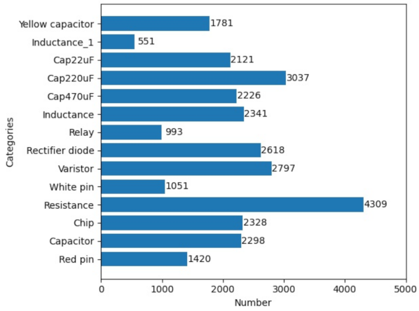
2.1. Multi-Scene Electronic Component Dataset
2.2. Public Datasets
3. Method
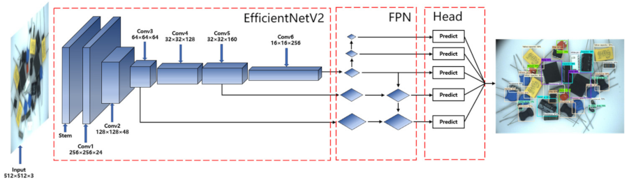
3.1. Efficientnetv2
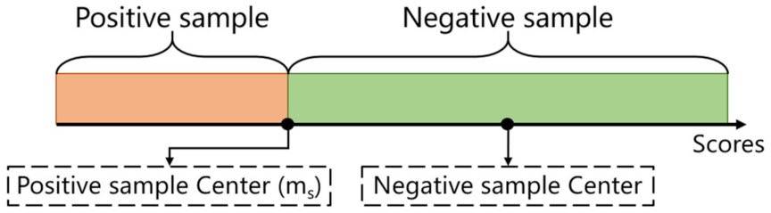
3.2. Adaptive Positive and Negative Sample Matching Strategy
| Algorithm 1. K-Means-based anchor assignment algorithm. |
| Input:, , , , G is a set of ground truth boxes on the image A is a set of all anchor boxes is a set of all anchor boxes from the pyramid levels L is the number of feature pyramid levels K is the number of candidate anchors for each pyramid Output: , is a set of positive samples is a set of negative samples 1: for each ground-truth do 2: Get the best ground truth with among all anchors by IoU 3: for each level ] do 4: 5: Calculate the loss score of 6: FindKthSmallest(, ) 7: 8: end for 9: 10: 11: The score in is less than or equal 12: The score in is greater than 13: , 14: end for 15: return , |
3.3. The Proposed Algorithm
4. Experiments and Discussion
4.1. Evaluation Criteria
4.1.1. Precision and Recall
4.1.2. AP and mAP
4.1.3. Params and Flops
4.2. Comparison of Different Algorithms
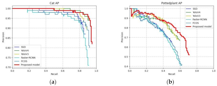
4.2.1. Comparison of Public Datasets
4.2.2. Comparison of Multi-Scene Electronic Component Datasets
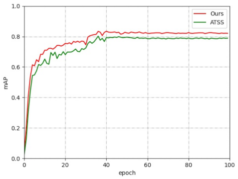
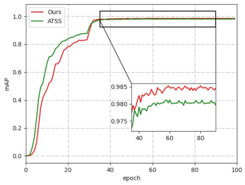
4.3. The Influence of Positive and Negative Sample Matching Strategies
5. Conclusions
Author Contributions
Funding
Institutional Review Board Statement
Informed Consent Statement
Data Availability Statement
Conflicts of Interest
References
- Wang, W.; Zhang, Y.; Gu, J.; Wang, J. A Proactive Manufacturing Resources Assignment Method Based on Production Performance Prediction for the Smart Factory. IEEE Trans. Ind. Inform. 2022, 18, 46–55. [Google Scholar] [CrossRef]
- Fu, L.; Zhang, Y.; Huang, Q.; Chen, X. Research and Application of Machine Vision in Intelligent Manufacturing. In Proceedings of the 2016 Chinese Control and Decision Conference (CCDC), Yinchuan, China, 28–30 May 2016; pp. 1126–1131. [Google Scholar]
- Ren, S.; He, K.; Girshick, R.; Sun, J. Faster R-CNN: Towards Real-Time Object Detection with Region Proposal Networks. IEEE Trans. Pattern Anal. Mach. Intell. 2017, 39, 1137–1149. [Google Scholar] [CrossRef] [PubMed] [Green Version]
- Girshick, R.; Jeff, D.; Trevor, D.; Malik, J. Rich Feature Hierarchies for Accurate Object Detection and Semantic Segmentation. In Proceedings of the IEEE Conference on Computer Vision and Pattern Recognition, Columbus, OH, USA, 23–28 June 2014; pp. 580–587. [Google Scholar]
- Girshick, R. Fast R-CNN. In Proceedings of the IEEE International Conference on Computer Vision, Las Vegas, NV, USA, 27–30 June 2015; pp. 1440–1448. [Google Scholar]
- Liu, W.; Anguelov, D.; Erhan, D.; Szegedy, C.; Reed, S.; Fu, C.Y.; Berg, A.C. SSD: Single Shot Multibox Detector. In Proceedings of the European Conference on Computer Vision, Amsterdam, The Netherlands, 8–16 October 2016; Volume 9905 LNCS, pp. 21–37. [Google Scholar]
- Redmon, J.; Divvala, S.; Girshick, R.; Farhadi, A. You Only Look Once: Unified, Real-Time Object Detection. In Proceedings of the IEEE Computer Society Conference on Computer Vision and Pattern Recognition, Las Vegas, NV, USA, 27–30 June 2016. [Google Scholar]
- Redmon, J.; Farhadi, A. YOLO9000: Better, Faster, Stronger. In Proceedings of the 2017 IEEE Conference on Computer Vision and Pattern Recognition (CVPR), Honolulu, Hawaii, 22–25 July 2017; pp. 6517–6525. [Google Scholar]
- Redmon, J.; Farhadi, A. YOLOv3: An Incremental Improvement. arXiv 2018, arXiv:1804.02767. [Google Scholar]
- Bochkovskiy, A.; Wang, C.-Y.; Liao, H.-Y.M. YOLOv4: Optimal Speed and Accuracy of Object Detection. arXiv 2020, arXiv:2004.10934. [Google Scholar]
- Lin, T.Y.; Dollár, P.; Girshick, R.; He, K.; Hariharan, B.; Belongie, S. Feature Pyramid Networks for Object Detection. In Proceedings of the IEEE Conference on Computer Vision and Pattern Recognition, Honolulu, HI, USA, 21–26 July 2017; pp. 2117–2125. [Google Scholar]
- Lin, T.Y.; Goyal, P.; Girshick, R.; He, K.; Dollar, P. Focal Loss for Dense Object Detection. IEEE Trans. Pattern Anal. Mach. Intell. 2020, 42, 318–327. [Google Scholar] [CrossRef] [PubMed] [Green Version]
- Zhou, X.; Austin, U.T.; Wang, D.; Berkeley, U.C.; Austin, U.T. Objects as Points. arXiv 2019, arXiv:1904.07850. [Google Scholar]
- Law, H.; Deng, J. CornerNet: Detecting Objects as Paired Keypoints. In Proceedings of the European Conference on Computer Vision (ECCV), Munich, Germany, 8–14 September 2018; Volume 128, pp. 734–750. [Google Scholar]
- Tian, Z.; Shen, C.; Chen, H.; He, T. FCOS: Fully Convolutional One-Stage Object Detection. In Proceedings of the IEEE/CVF International Conference on Computer Vision, Seoul, Korea, 27 October–2 November 2019; pp. 9627–9636. [Google Scholar]
- Zhang, S.; Chi, C.; Yao, Y.; Lei, Z.; Li, S.Z. Bridging the Gap between Anchor-Based and Anchor-Free Detection via Adaptive Training Sample Selection. In Proceedings of the IEEE Computer Society Conference on Computer Vision and Pattern Recognition, Seattle, WA, USA, 14–19 June 2020; pp. 9759–9768. [Google Scholar]
- Kim, K.; Lee, H.S. Probabilistic Anchor Assignment with IoU Prediction for Object Detection. In Proceedings of the Computer Vision—ECCV 2020: 16th European Conference, Glasgow, UK, 23–28 August 2020; Volume 12370 LNCS, pp. 355–371. [Google Scholar]
- Simonyan, K.; Zisserman, A. Very Deep Convolutional Networks for Large-Scale Image Recognition. arXiv 2014, arXiv:1409.1556. [Google Scholar]
- Szegedy, C.; Liu, W.; Jia, Y.; Sermanet, P.; Reed, S.; Anguelov, D.; Erhan, D.; Vanhoucke, V.; Rabinovich, A. Going Deeper with Convolutions. In Proceedings of the IEEE Conference On Computer Vision And Pattern Recognition, Boston, MA, USA, 7–12 June 2015; pp. 1–9. [Google Scholar]
- He, K.; Zhang, X.; Ren, S.; Sun, J. Deep Residual Learning for Image Recognition. In Proceedings of the IEEE Conference on Computer Vision and Pattern Recognition, Las Vegas, NV, USA, 26 June–1 July 2016; pp. 770–778. [Google Scholar]
- Hu, J.; Shen, L.; Albanie, S.; Sun, G.; Wu, E. Squeeze-and-Excitation Networks. IEEE Trans. Pattern Anal. Mach. Intell. 2020, 42, 2011–2023. [Google Scholar] [CrossRef] [PubMed] [Green Version]
- Howard, A.G.; Zhu, M.; Chen, B.; Kalenichenko, D.; Wang, W.; Weyand, T.; Andreetto, M.; Adam, H. MobileNets: Efficient Convolutional Neural Networks for Mobile Vision Applications. arXiv 2017, arXiv:1704.04861. [Google Scholar]
- Sandler, M.; Howard, A.; Zhu, M.; Zhmoginov, A.; Chen, L.-C. Inverted Residuals and Linear Bottlenecks Mark. In In Proceedings of the IEEE Conference on Computer Vision and Pattern Recognition, Salt Lake City, UT, USA, 18–23 June 2018; pp. 4510–4520. [Google Scholar]
- Howard, A.; Sandler, M.; Chen, B.; Wang, W.; Chen, L.C.; Tan, M.; Chu, G.; Vasudevan, V.; Zhu, Y.; Pang, R.; et al. Searching for MobileNetV3. In Proceedings of the IEEE/CVF International Conference on Computer Vision, Seoul, Korea, 27–28 October 2019; pp. 1314–1324. [Google Scholar]
- Zhang, X.; Zhou, X.; Lin, M.; Sun, J. ShuffleNet: An Extremely Efficient Convolutional Neural Network for Mobile Devices. In Proceedings of the IEEE Conference on Computer Vision and Pattern Recognition, Salt Lake City, UT, USA, 18–23 June 2018; pp. 6848–6856. [Google Scholar]
- Ma, N.; Zhang, X.; Zheng, H.-T.; Sun, J. ShuffleNet V2: Practical Guidelines for Efficient CNN Architecture Design. In Proceedings of the European Conference on Computer Vision (ECCV), Munich, Germany, 8–14 September 2018; Volume 11218 LNCS, pp. 116–131. [Google Scholar]
- Radosavovic, I.; Kosaraju, R.P.; Girshick, R.; He, K.; Dollár, P. Designing Network Design Spaces. In Proceedings of the IEEE/CVF Conference on Computer Vision and Pattern Recognition, Seattle, WA, USA, 14–19 June 2020; pp. 10428–10436. [Google Scholar]
- Tan, M.; Le, Q.v. EfficientNet: Rethinking Model Scaling for Convolutional Neural Networks. In Proceedings of the International Conference on Machine Learning, Long Beach, CA, USA, 10–15 June 2019; pp. 6105–6114. [Google Scholar]
- Tan, M.; Le, Q.v. EfficientNetV2: Smaller Models and Faster Training. In Proceedings of the International Conference on Machine Learning, Jeju, Korea, 23–25 April 2021. [Google Scholar]
- Kuo, C.-W.; Ashmore, J.; Huggins, D.; Kira, Z. Data-Efficient Graph Embedding Learning for PCB Component Detection. In Proceedings of the 2019 IEEE Winter Conference on Applications of Computer Vision (WACV), Waikoloa Village, HI, USA, 7–11 January 2019; pp. 551–560. [Google Scholar]
- Sun, X.; Gu, J.; Huang, R. A Modified SSD Method for Electronic Components Fast Recognition. Optik 2020, 205, 163767. [Google Scholar] [CrossRef]
- Huang, R.; Gu, J.; Sun, X.; Hou, Y.; Uddin, S. A Rapid Recognition Method for Electronic Components Based on the Improved YOLO-V3 Network. Electronics 2019, 8, 825. [Google Scholar] [CrossRef] [Green Version]
- Li, J.; Gu, J.; Huang, Z.; Wen, J. Application Research of Improved YOLO V3 Algorithm in PCB Electronic Component Detection. Appl. Sci. 2019, 9, 3750. [Google Scholar] [CrossRef] [Green Version]
- Yang, Z.; Dong, R.; Xu, H.; Gu, J. Instance Segmentation Method Based on Improved Mask R-Cnn for the Stacked Electronic Components. Electronics 2020, 9, 886. [Google Scholar] [CrossRef]
- Li, J.; Li, W.; Chen, Y.; Gu, J. A PCB Electronic Components Detection Network Design Based on Effective Receptive Field Size and Anchor Size Matching. Comput. Intell. Neurosci. 2021, 2021, 6682710. [Google Scholar] [CrossRef] [PubMed]
- Everingham, M.; van Gool, L.; Williams, C.K.I.; Winn, J.; Zisserman, A. The Pascal Visual Object Classes (VOC) Challenge. Int. J. Comput. Vis. 2010, 88, 303–338. [Google Scholar] [CrossRef] [Green Version]
- Padilla, R.; Passos, W.L.; Dias, T.L.B.; Netto, S.L.; da Silva, E.A.B. A Comparative Analysis of Object Detection Metrics with a Companion Open-Source Toolkit. Electronics 2021, 10, 279. [Google Scholar] [CrossRef]


| Name | Image | Name | Image |
|---|---|---|---|
| Cap22uF |  | Cap220uF |  |
| Inductance_1 |  | Cap470uF |  |
| Resistance |  | Capacitor |  |
| Red pin |  | Varistor |  |
| Chip |  | Rectifier diode |  |
| Inductance | 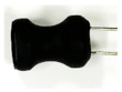 | Yellow capacitor |  |
| White pin | 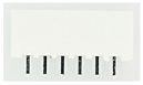 | Relay | 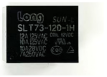 |
| Model | FLOPs | Params | mAP |
|---|---|---|---|
| SSD | 90.54 | 26.42 M | 71.44% |
| Faster RCNN | 461.76 | 28.48 M | 76.84% |
| YOLOV3 | 49.7 | 61.59 M | 77.73% |
| YOLOV4 | 45.37 | 64.05 M | 80.49% |
| FCOS | 51.69 | 31.92 M | 76.18% |
| Proposed model | 44.26 | 29.3 M | 83.44% |
| Model | FLOPs | Params | mAP |
|---|---|---|---|
| SSD | 90.54 | 26.42 M | 95.67% |
| Faster RCNN | 461.76 | 28.48 M | 96.19% |
| YOLOV3 | 49.7 | 61.59 M | 97.98% |
| YOLOV4 | 45.37 | 64.05 M | 88.40% |
| FCOS | 51.69 | 31.92 M | 98.24% |
| Huang | 15.46 | 25.24 | 95.76% |
| Li | 53.97 | 61.86 | 88.56% |
| Proposed model | 44.26 | 29.3 M | 98.83% |
| Proposed model | 82.89% |
| Proposed model + ATSS | 81.62% |
| Proposed model | 98.83% |
| Proposed model + ATSS | 98.67% |
Publisher’s Note: MDPI stays neutral with regard to jurisdictional claims in published maps and institutional affiliations. |
© 2022 by the authors. Licensee MDPI, Basel, Switzerland. This article is an open access article distributed under the terms and conditions of the Creative Commons Attribution (CC BY) license (https://creativecommons.org/licenses/by/4.0/).
Share and Cite
Xia, Z.; Gu, J.; Zhang, K.; Wang, W.; Li, J. Research on Multi-Scene Electronic Component Detection Algorithm with Anchor Assignment Based on K-Means. Electronics 2022, 11, 514. https://doi.org/10.3390/electronics11040514
Xia Z, Gu J, Zhang K, Wang W, Li J. Research on Multi-Scene Electronic Component Detection Algorithm with Anchor Assignment Based on K-Means. Electronics. 2022; 11(4):514. https://doi.org/10.3390/electronics11040514
Chicago/Turabian StyleXia, Zilin, Jinan Gu, Ke Zhang, Wenbo Wang, and Jing Li. 2022. "Research on Multi-Scene Electronic Component Detection Algorithm with Anchor Assignment Based on K-Means" Electronics 11, no. 4: 514. https://doi.org/10.3390/electronics11040514
APA StyleXia, Z., Gu, J., Zhang, K., Wang, W., & Li, J. (2022). Research on Multi-Scene Electronic Component Detection Algorithm with Anchor Assignment Based on K-Means. Electronics, 11(4), 514. https://doi.org/10.3390/electronics11040514