
A Method for Evaluating the Maximum Capacity of Grid-Connected Wind Farms Considering Multiple Stability Constraints


Abstract
:1. Introduction
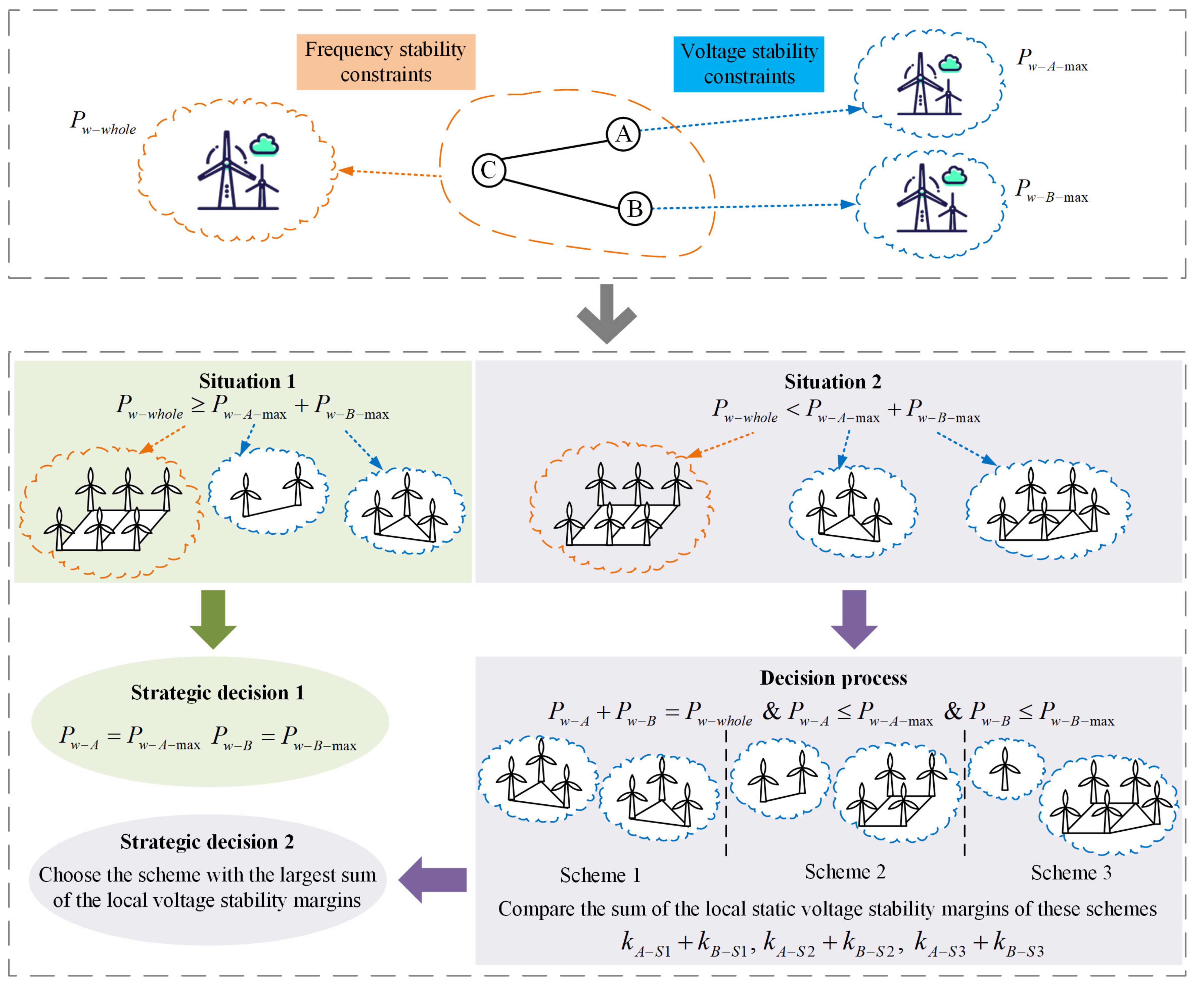
2. Overall Scheme
- (a)
- Obtain the maximum capacity of grid-connected wind farms of the whole power grid. The solution proposed in this work is to assess the maximum capacity of grid-connected wind farms of the whole power grid based on the frequency stability constraints;
- (b)
- Obtain the maximum capacity of grid-connected wind farms of each local power grid. The solution proposed is to evaluate the maximum capacity of grid-connected wind farms of the local power grids A and B, expressed as and , based on the voltage stability constraints. Thus, the sum of them is obtained as:
- (c)
- Quantitatively assess the capacity of grid-connected wind farms of each local power grid. The solution proposed is as follows: if the maximum capacity of grid-connected wind farms of the whole power grid is no less than the sum of the capacity of grid-connected wind farms of all local power grids, i.e., , then the local power grids can be integrated with wind farms according to their maximum capacity respectively. In Figure 1, it is supposed that and are the ultimately determined values of the capacity of grid-connected wind farms of the local power grids A and B. Then the strategic decision can be made that , . In the opposite situation, i.e., , under the constraint of the maximum capacity of grid-connected wind farms of the whole power grid, the capacity of grid-connected wind farms of each local power grid needs to be quantitatively assessed based on the correlation between the local static voltage stability margin and the local capacity of grid-connected wind farms. That is, the sum of the capacity of grid-connected wind farms of all local power grids being equal to the maximum capacity of the whole power grid is seen as the constraint condition, and the sum of the static voltage stability margins of all local power grids reaching its maximum value is regarded as the optimization objective. At last, the quantitative assessment results of the capacity of each local power grid are solved. In Figure 1, for example, there are three different schemes in which the sum of the capacity of grid-connected wind farms of the local power grids A and B is equal to the maximum capacity of the whole power grid. It is assumed that and are the static voltage stability margins of the local power grids A and B in scheme 1 respectively. Similarly, and are the static voltage stability margins in scheme 2, and and are the static voltage stability margins in scheme 3. Then we compare the sums of the static voltage stability margins in all the schemes and choose the scheme with the largest sum as the ultimate strategic decision.
3. Frequency and Voltage Stability Constraints
3.1. Frequency Stability Constraints
3.1.1. RoCoF Constraint
3.1.2. Steady-State Frequency Deviation Constraint
3.1.3. Maximum Transient Frequency Deviation Constraint
3.2. Voltage Stability Constraint
3.2.1. Static Voltage Constraint
- (1)
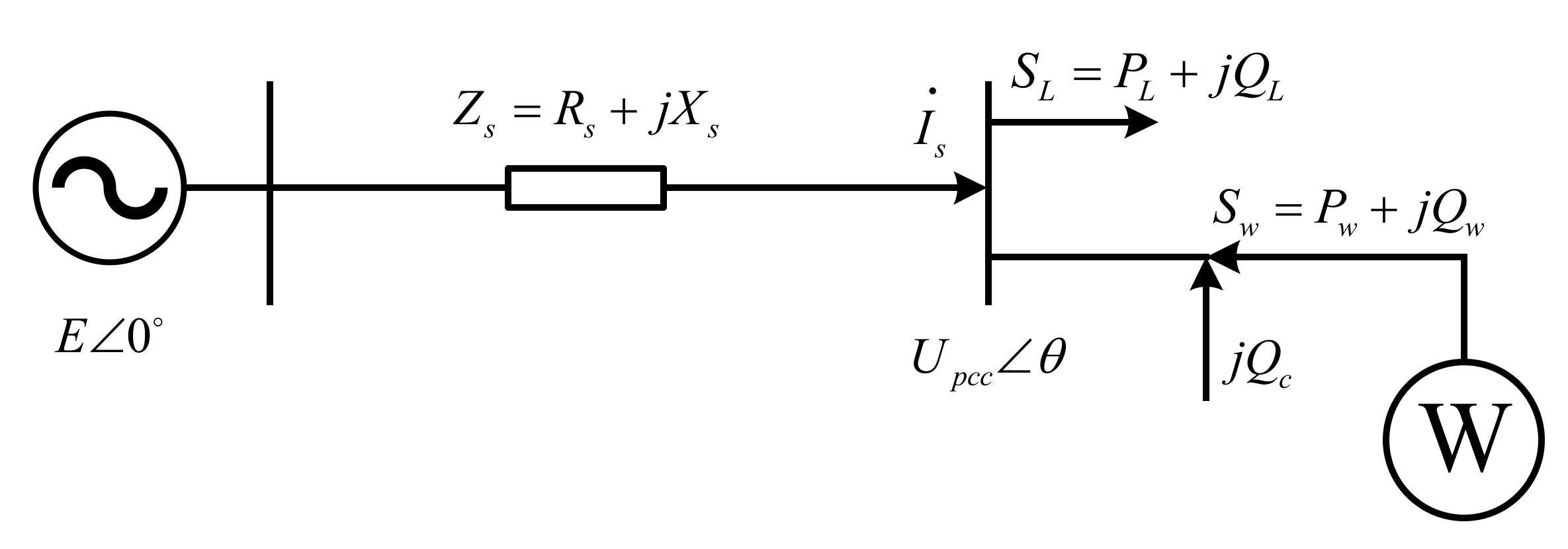
- Influence of wind farm integration on static voltage stability of the PCC
- (2)
- The calculation method of the static voltage stability margin
3.2.2. Transient Voltage Stability Constraint
3.3. Evaluation Results Based on the Constraints
4. Quantitative Assessment of the Capacity of Grid-Connected Wind Farms of Each Local Power Grid
- (1)
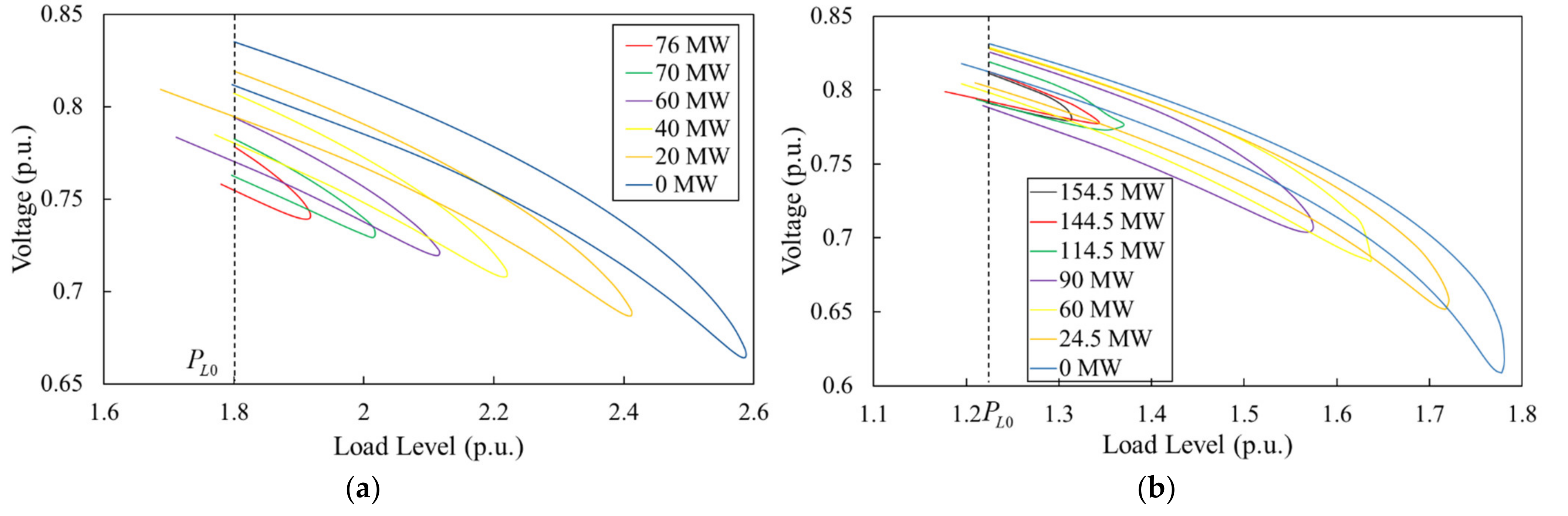
- The static voltage stability margins of each local power grid under different capacity values of are obtained by using the static voltage stability analysis module of the Power System Analysis Synthesis Program (PSASP) developed by the China Electric Power Research Institute. During the simulation, the adjusted power grid operating modes in accordance with the different capacity values of are the inputs for the static voltage stability analysis module of PSASP, while the corresponding static voltage stability margins are the outputs. After calculating multiple groups of data results of and , the approximate relational expression between and can be obtained. Thus the approximate curves can be fitted. According to reference [19], the curves are similar to those shown in Figure 3.
- (2)
- Set the constraint condition that the sum of the capacity of grid-connected wind farms of each local power grid is equal to the maximum capacity of the whole power grid, as expressed in Equation (25). Set the objective function that the sum of the static voltage stability margin of each local power grid reaches its maximum, as expressed in Equation (26).
- (3)
- Under the constraint condition of Equation (25), the objective function of Equation (26) is solved to obtain the quantitative assessment scheme of the capacity of grid-connected wind farms of the local power grids A and B respectively.
5. Method for Assessing the Maximum Capacity of Grid-Connected Wind Farms under the Joint Constraints of Frequency and Voltage Stability
- Step 1:
- Determine local power grids to be integrated with wind farms. The way of wind farm integration is that wind turbines replace synchronous generators of equal capacity.
- Step 2:
- Wind turbines are incrementally added to the whole power grid gradually, and set the tripping fault for the synchronous generator with the maximum output. Then use the transient stability program of PSASP for simulation calculations. When the system frequency just reaches the stability boundary of any one of the frequency stability constraints, take the capacity of grid-connected wind farms in this mode as the value of .
- Step 3:
- By using the static voltage stability analysis module of PSASP, the static voltage stability margin of each local power grid can be obtained separately. Gradually increase the quantity of wind turbines in the ith local power grid until the static voltage stability margin reaches the stability boundary of 8%, and a certain margin can be retained. The capacity of grid-connected wind farms in this mode is the value of . Accomplish the simulations for all the local power grids, and the sum of can be obtained, i.e., .
- Step 4:
- If , each local power grid can be integrated with wind farms according to .
- Step 5:
- If , the capacity of grid-connected wind farms of each local power grid needs to be quantitatively assessed. The static voltage stability margins of each local power grid under different capacity values of are obtained by using the static voltage stability analysis module of PSASP. Then the approximate relational expression between and can be obtained. Thus the approximate curves can be fitted.Set the constraint condition and the objective function respectively as:
- Step 6:
- After solving the objective function under the constraint condition, quantitatively assessing the capacity of grid-connected wind farms of the whole and each local power grid is accomplished.
6. Simulation Verification
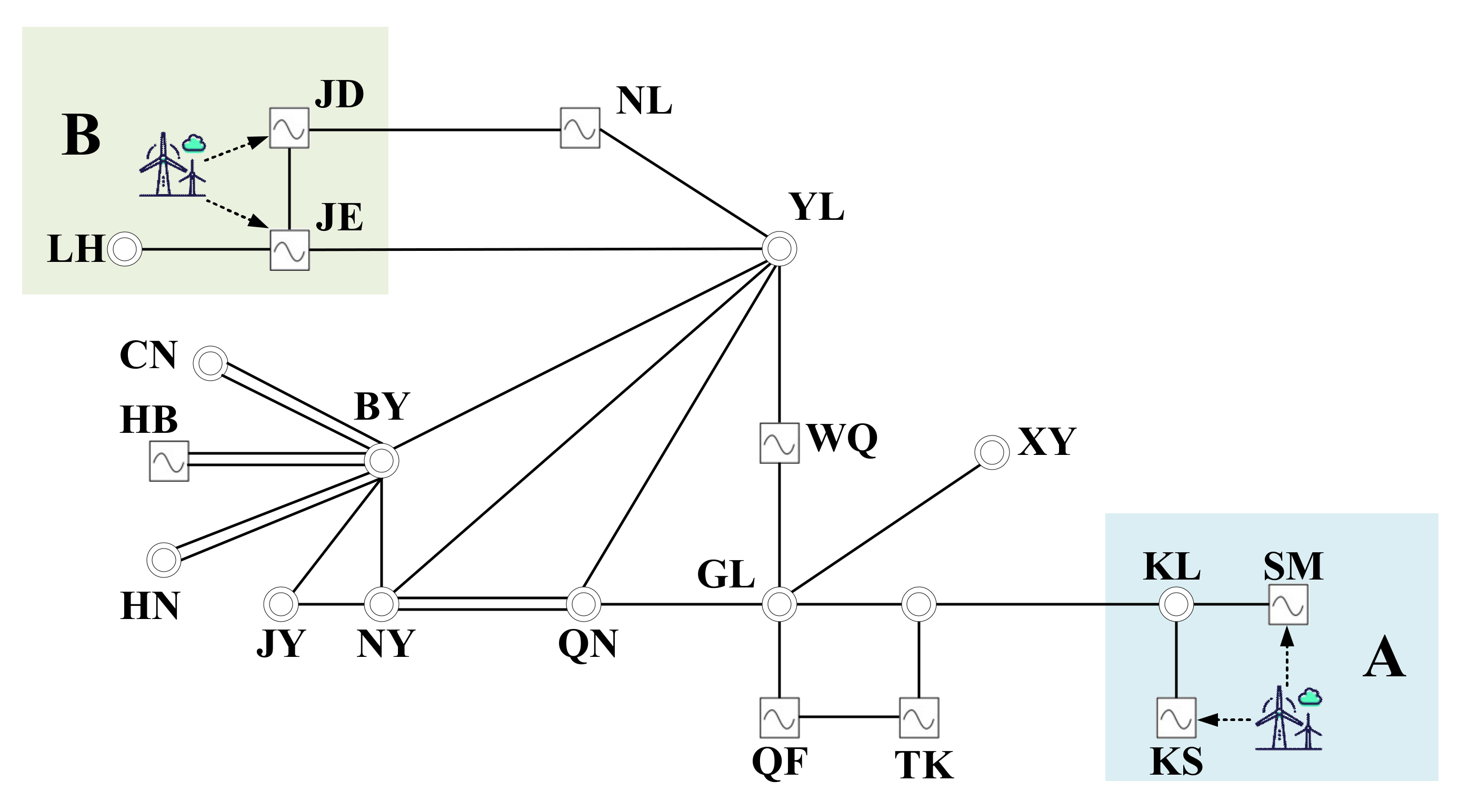
6.1. Introduction to the Power Grid
6.2. Maximum Capacity of Grid-Connected Wind Farms of the Whole Power Grid
6.3. Maximum Capacity of Grid-Connected Wind Farms of Each Local Power Grid
6.4. Quantitative Assessment of the Capacity of Grid-Connected Wind Farms of Each Local Power Grid
6.5. Contrastive Analysis of the Proposed Method and Other Methods
7. Conclusions
- (1)
- A large-scale integration of wind farms will have adverse effects on both the frequency and voltage stability of the power grid. The frequency stability limits the maximum capacity of grid-connected wind farms of the whole power grid, and the voltage stability limits the maximum capacity of grid-connected wind farms of each local power grid. It is the theoretical basis of the method proposed in this paper.
- (2)
- The quantitative assessment method proposed in this paper effectively solves the problem of how to quantitatively assess the capacity of grid-connected wind farms of each local power grid when the sum of the maximum capacity of grid-connected wind farms of each local power grid is greater than the maximum capacity of the whole power grid. Meanwhile, the static voltage stability margins of the local power grids can be maintained at a high level.
- (3)
- In combination with the frequency and voltage stability problems mainly faced by modern power systems, the maximum capacity of grid-connected wind farms of the power grid is assessed. However, in some cases, the maximum capacity of grid-connected wind farms may also be constrained by other stability constraints, such as the thermal stability constraint, the power angle stability constraint, etc. What is more, there are other difficult issues in the research such as how to decouple the power angle instability mode and the transient voltage instability mode. In future work, the method for evaluating the maximum capacity of grid-connected wind farms including other stability constraints will be further studied.
Author Contributions
Funding
Conflicts of Interest
References
- Global Wind Report 2021. Available online: https://gwec.net/global-wind-report-2021/ (accessed on 25 March 2021).
- Gevorgian, V.; Zhang, Y.; Ela, E. Investigating the impacts of wind generation participation in interconnection frequency response. IEEE Trans. Sustain. Energy 2017, 6, 1004–1012. [Google Scholar] [CrossRef]
- Martínez-Lucas, G.; Sarasúa, J.I.; Pérez-Díaz, J.I.; Martínez, S.; Ochoa, D. Analysis of the implementation of the primary and/or inertial frequency control in variable speed wind turbines in an isolated power system with high renewable penetration. Case Study: El Hierro Power System. Electronics 2020, 9, 901. [Google Scholar] [CrossRef]
- Dai, J.; Tang, Y.; Yi, J. Adaptive gains control scheme for PMSG-based wind power plant to provide voltage regulation service. Energies 2019, 12, 753. [Google Scholar] [CrossRef] [Green Version]
- Nguyen, N.; Mitra, J. An analysis of the effects and dependency of wind power penetration on system frequency regulation. IEEE Trans. Sustain. Energy 2015, 7, 354–363. [Google Scholar] [CrossRef]
- Yu, H.Y.; Bansal, R.C.; Dong, Z.Y. Fast computation of the maximum wind penetration based on frequency response in small isolated power systems. Appl. Energy 2014, 113, 648–659. [Google Scholar] [CrossRef]
- Yan, R.; Saha, T.K.; Modi, N.; Masood, N.A.; Mosadeghy, M. The combined effects of high penetration of wind and pv on power system frequency response. Appl. Energy 2015, 145, 320–330. [Google Scholar] [CrossRef]
- Dai, J.; Tang, Y.; Wang, Q. Fast method to estimate maximum penetration level of wind power considering frequency cumulative effect. IET Gener. Transm. Distrib. 2019, 13, 1726–1733. [Google Scholar] [CrossRef]
- O’Sullivan, J.; Rogers, A.; Flynn, D.; Smith, P.; Mullane, A.; O’Malley, M. Studying the maximum instantaneous non-synchronous generation in an island system—frequency stability challenges in Ireland. IEEE Trans. Power Syst. 2018, 33, 985–994. [Google Scholar] [CrossRef] [Green Version]
- Masood, N.A.; Yan, R.; Saha, T.K. A new tool to estimate maximum wind power penetration level: In perspective of frequency response adequacy. Appl. Energy 2015, 154, 209–220. [Google Scholar] [CrossRef]
- Gil-González, W.; Montoya, O.D.; Escobar-Mejía, A.; Hernández, J.C. LQR-Based adaptive virtual inertia for grid integration of wind energy conversion system based on synchronverter model. Electronics 2021, 10, 1022. [Google Scholar] [CrossRef]
- Li, T.; Wang, L.; Wang, Y.; Liu, G.; Zhu, Z.; Zhang, Y.; Zhao, L.; Ji, Z. Data-driven virtual inertia control method of doubly fed wind turbine. Energies 2021, 14, 5572. [Google Scholar] [CrossRef]
- Xu, B.; Zhang, L.; Yao, Y.; Yu, X.; Yang, Y.; Li, D. Virtual inertia coordinated allocation method considering inertia demand and wind turbine inertia response capability. Energies 2021, 14, 5002. [Google Scholar] [CrossRef]
- Krpan, M.; Kuzle, I. Dynamic characteristics of virtual inertial response provision by DFIG-based wind turbines. Electr. Power Syst. Res. 2020, 178, 106005. [Google Scholar] [CrossRef]
- Vittal, E.; O’Malley, M.; Keane, A. A steady-state voltage stability analysis of power systems with high penetrations of wind. IEEE Trans. Power Syst. 2010, 25, 433–442. [Google Scholar] [CrossRef]
- He, H.; Zhang, Y.; Sun, X.; Guo, Q.; Su, L.; Wang, Y.; Wang, M.; Huang, B. Evaluation method of renewable energy development scale and DC transmission scale of China Northwest power grid by considering frequency security constraints. Proc. CSEE 2021, 41, 4753–4762. [Google Scholar]
- Burchett, S.; Douglas, D.; Ghiocel, S.G.; Liehr, M.; Chow, J.H.; Kosterev, D.; Faris, A.; Heredia, E.; Matthews, G.H. An optimal Thévenin equivalent estimation method and its application to the voltage stability analysis of a wind hub. IEEE Trans. Power Syst. 2018, 33, 3644–3652. [Google Scholar] [CrossRef]
- Tang, Y.; Chang, P.; Dai, J.; Yi, J.; Lin, W.; Yu, F. Evaluation method of maximum wind penetration level considering static voltage stability constraint. In Proceedings of the 2020 IEEE International Conference on Power Systems Technology (POWERCON), No.5, 11th Cross, 2nd Stage, West of Chord Road, Bangalore, Karnataka, India, 14–16 September 2020. [Google Scholar]
- Yi, J.; Lin, W.; Yu, F.; Lin, A.; Yang, F. Calculation method of critical penetration of renewable energy constrained by static voltage stability. Power Syst. Tech. 2020, 44, 2906–2912. [Google Scholar]


| Local Power Grid | Capacity of Grid-Connected Wind Farms (MW) | Load Node | |||
|---|---|---|---|---|---|
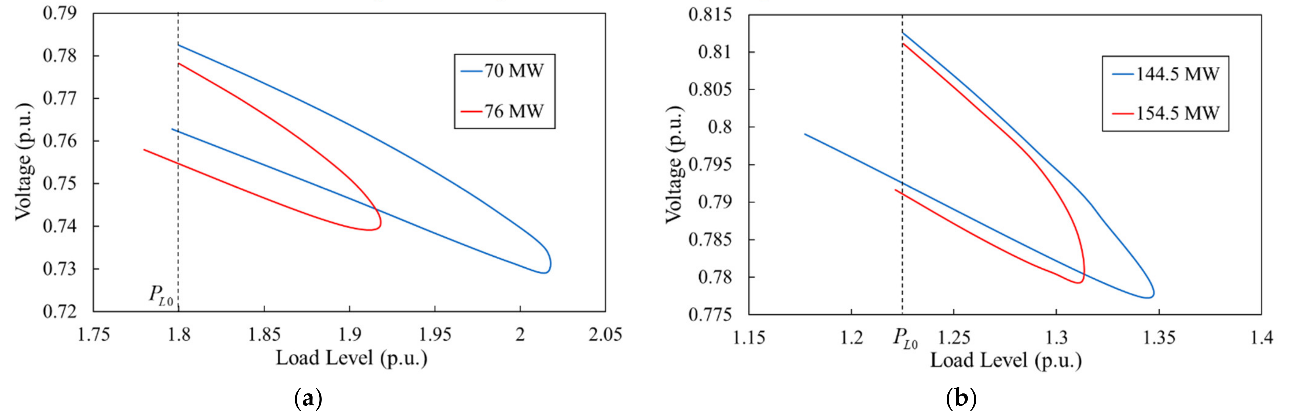
| A | 70 | KL | 180 | 201.538 | 11.97% |
| 76 | 180 | 191.739 | 6.52% | ||
| B | 144.5 | LH | 122.52 | 134.035 | 9.40% |
| 154.5 | 122.52 | 131.268 | 7.14% |
Publisher’s Note: MDPI stays neutral with regard to jurisdictional claims in published maps and institutional affiliations. |
© 2022 by the authors. Licensee MDPI, Basel, Switzerland. This article is an open access article distributed under the terms and conditions of the Creative Commons Attribution (CC BY) license (https://creativecommons.org/licenses/by/4.0/).
Share and Cite
Wu, X.; Xue, F.; Tang, Y.; Dai, J. A Method for Evaluating the Maximum Capacity of Grid-Connected Wind Farms Considering Multiple Stability Constraints. Electronics 2022, 11, 509. https://doi.org/10.3390/electronics11040509
Wu X, Xue F, Tang Y, Dai J. A Method for Evaluating the Maximum Capacity of Grid-Connected Wind Farms Considering Multiple Stability Constraints. Electronics. 2022; 11(4):509. https://doi.org/10.3390/electronics11040509
Chicago/Turabian StyleWu, Xingyang, Feng Xue, Yi Tang, and Jianfeng Dai. 2022. "A Method for Evaluating the Maximum Capacity of Grid-Connected Wind Farms Considering Multiple Stability Constraints" Electronics 11, no. 4: 509. https://doi.org/10.3390/electronics11040509
APA StyleWu, X., Xue, F., Tang, Y., & Dai, J. (2022). A Method for Evaluating the Maximum Capacity of Grid-Connected Wind Farms Considering Multiple Stability Constraints. Electronics, 11(4), 509. https://doi.org/10.3390/electronics11040509