A Comparison of Distribution Models for Fast Variations in the Indoor Radio Channel at 5G Frequency Range 1 Microwave Bands

Abstract

The use of long-term (slow variations) for modelling radio propagation behavior in indoor scenarios limits the validity of such models, as most of the environments induced fast variations overlapped with the slow ones. Real world data gathered at different locations in two bands within Fifth Generation FR1 spectrum, 3 GHz and 5 GHz, provide insight on the effect of such fast variations and on the distribution models that would be useful to complement the long term analysis with short term behavior in order to improve the design of such 5G microwave networks. Comparisons among short term performance taking into account both the frequency, the visibility conditions and the environment size, shape and furnishing are presented with the focus on modelling as accurate as possible the narrowband channel. The use of ΔBIC (describing the difference between Bayesian Information Criteria indexes of each fitting) complements and confirms the insight provided by direct inspection on traditional fitting plots. This parameter could be interesting for future network deployments.

1. Introduction

The radio channel governs the performance of any wireless system deployed on it. Additionally, this also occurs, of course, for all new proposals regarding the fifth generation (5G) of cellular mobile communications and all its related applications: Internet of Things, augmented reality, smart cities, smart houses, etc. [1]. Variations or instabilities of the radio channel could affect the performance of some of these known 5G applications, and probably many of those that will arise in the following years, at different levels. Then, modeling the underlying propagation channels boosts the deployment of such technologies [2]. Additionally, among the different characteristics of the propagation channel, modeling the multipath fading emerges as one of the key elements.

Fading events limit the performance of radio communication systems, and then its characterization and prediction have targeted the research for a long time [3,4]. Depending on the application, this effect could dramatically limit the effective usefulness, i.e., when trying to provide positioning by using receiving power from different base stations as a measure of distance [5]. In this case, errors in signal amplitude induced by fast fading events would lead to errors in distance computation, and then in errors in positioning when computing the triangles for coordinate calculations. As with this example, many other 5G-supported applications would suffer the fast fading effects to different limits, even being catastrophic. Thus, having valid models on fading activity helps the new deployments for that and many other applications. Commonly, such models include two types of fading: large-scale or slow fading (mainly shadowing and path loss) and small-scale or fast fading [6,7]. There were some attempts to deterministically predict the appearance and duration of such effects [8], but the amount of possible interference sources or scattering obstacles put the focus on their statistical analysis.

A good statistical channel characterization represents a first step for improving the performance of OFDM systems regarding the mitigation of induced inter-carrier interference [9,10], with direct influence in the perceived quality of service provided by 5G-based applications. With the advent of cognitive radio proposals, statistically defined fast-fading became useful for cases in which the systems would need to estimate the radio channel behavior [11]: the non-deterministic behavior is commonly more complex to estimate, and depending on the depth of the fading, it could be crucial for the success of the system. Thus, Rayleigh fast fading is commonly used for outdoor propagation [12], the modelling of which is habitually less complex than indoors. However, indoor propagation seems to follow a wider variety of statistical functions. Then, the fast-fading studies keep an open interest, as they have direct influence on capacity assessment [13].

The analysis of distribution models for the 2.4 GHz band was often discussed. In this band, studies of the distribution models that define fading variations have been applied to improve the precision of indoor positioning applications based on Bluetooth standards [5]. In this case, Weibull distribution arises as the most convenient to model the received signal strength indication (RSSI) for such band and indoor environments. Triangulation-location based on WiFi signals, also in the 2.4 GHz band, are analyzed by [14], using again the Weibull model for predicting indoor fast variations in the signal level. There are other alternative strategies for such location applications [15], but they are out of the scope of this proposal.

The interest of investigating the short term behavior for different applications at frequencies assigned to other previous wireless standards gives a chance to analogous research for the 5G technology band to be also valuable. Recent works have been published regarding channel characterization using ray-tracing for performing predictions at 3 GHz bands [16], which is one of the bands of interest in 5G. However, there are some effects that cannot be predicted by deterministic methods, due to their inherent statistical nature, as this is the aim of the presented work.

Along this paper, we analyze the behavior of fast-fading events observed in data gathered by means of large measurement campaigns in a variety of indoor environments. The focus was put on two frequency bands, one around 3.5 GHz and the other around 5.8 GHz, both within the microwave FR1 spectrum for 5G. From the measured data, we extracted the narrowband responses and then separated the slow and fast variations. These fast variations are modelled by means of different statistical functions, selecting those that best fit the measured data. The parameter ΔBIC (describing the difference between Bayesian Information Criteria indexes of each fitting) appears as a way to numerically compare pairs of different statistical distributions by the goodness of fit they provide. The results given by ΔBIC are observed by direct inspection of fitting plots, concluding that they offer good insight on the performance of the various considered models.

Weibull or Nakagami distributions reasonably describe most of the short-term variations on the indoor channel responses in the band around 3.5 GHz; whereas many other distributions seem accurate in the 5.8 GHz band. This trend linked the previously published results at lower [5,14] and higher frequencies [17,18,19]. Thus, this paper completes a knowledge gap, providing information regarding the distributions that best fit real world data, but also checking the use of a clear criteria for selecting them.

This insight is valuable for planning indoor coverages taking into account the different applications supported by 5G (both current and upcoming or even unknown applications) because in short latency high capacity links, the stability of the connectivity should be guaranteed. The special characteristics of 5G technology, which opens the door to new opportunities and applications, require knowledge for planning networks that are very stable, and this includes the application of guard intervals to absorb the non-deterministic modeled effects, as fast fading could be.

After this introduction, the second section shows the measurement environments and describes the setup and the procedure for performing the measurements. It also includes the basics of the processing applied to the measured data. The third section contains the results obtained after processing the gathered outcomes. These results are commented and compared at the fourth section. Finally, the fifth section summarizes the conclusions of the research.

2. Materials and Methods

This section describes the experiments performed to obtain the measured data, as well as the mathematical processing applied to that to select the distribution that better fits the short-term variability of radio channel responses. After the explanation of the measurement setup and the procedure, the different indoor environments are described, followed by the processing techniques.

2.1. Measurement Procedure

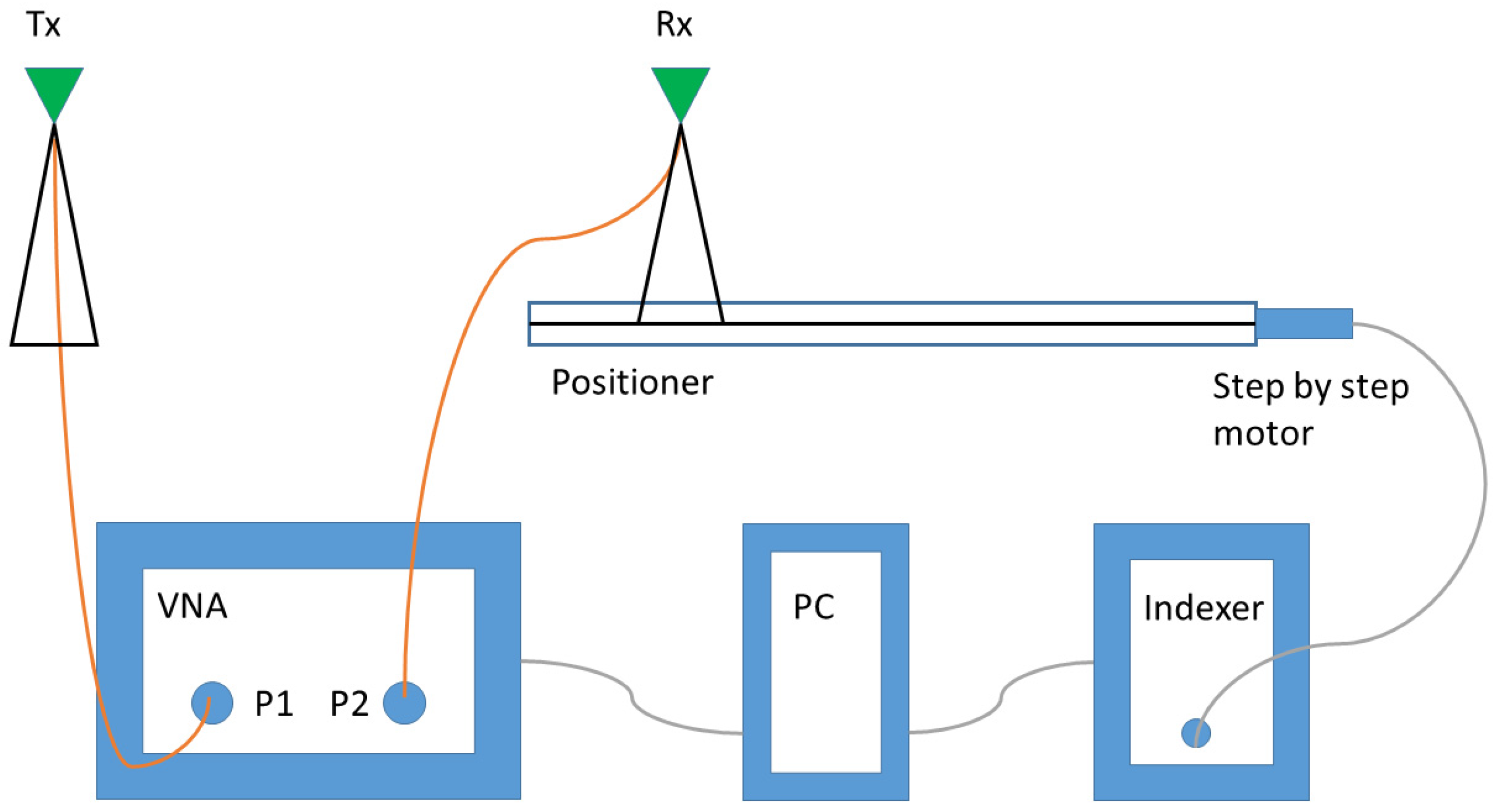
The measurement setup grew around a vector network analyzer (VNA), as schematized at Figure 1. The VNA worked as transmitter and receiver, and provided frequency responses of the radio channel by measuring the scattering parameter S₂₁, in module and phase format sweeping a spectrum band around the central frequency. Both antennas were azimuth-omnidirectional EM-6865 manufactured by Electro-Metrics. The transmitting antenna, connected to port 1 of the VNA, was placed in a static location, and it is represented in Figure 1 as a green triangle. The receiving antenna (another green triangle at Figure 1) was moving along a positioner, following a 2.5-m-long straight path. An indexer drove the step by step motor that controlled the movement along the positioner; thus, the location of the receiving antenna at each measurement spot is meticulously defined anytime. A tailor made software, based on Matlab^® and running on a PC, governed the process of both the movement and the electromagnetic equipment: this allows the repetition of the experiments reducing the human errors during the measurement campaigns.

Measurements followed a “stop-measure-move” iterative procedure, gathering averaged channel responses at each receiving spot, which was separated one eighth of wavelength from the previous adjacent one. This distance is selected to have uncorrelated samples, as well as to not lose possible multipath effects [20]. Once the receiving antenna reached a measurement spot, the movement stopped and the VNA performed the gathering of a radio channel frequency response around the central frequency. Then, the receiving antenna is moved to the next spot and the procedure is applied again. As the channel responses are measured as the relation between received power and transmitted power, calibrated by the “thru” procedure to the antenna connectors, data is non-dimensional and thus it is provided in dB.

For the 3 GHz band measurements, the VNA was an Agilent Fieldfox N9913A. The output power was fixed in 3 dBm and the receiver IF bandwidth in 10 kHz; an averaging of 10 frequency sweeps was selected to reduce the noise. We gathered data within a band between 3.35 and 3.65 GHz, in a 300 MHz wide bandwidth. A number of 1001 frequency samples at each frequency swept defined the complex frequency responses provided by the VNA. The lengths of the straight line paths vary depending on the scenario, as both auditorium and corridor are long enough to place the receiver positioner in several positions along an axis. A total number of 2100 measurement spots were explored, gathering 2,102,100 complex samples during the 3 GHz measurement campaign.

On the other hand, the VNA used during the 5 GHz band campaign was a Hewlett Packard 8510-C. The output power was fixed at 10 dBm. Besides, a 20 dB gain amplifier Mini Circuits model ZRON-8G was used for a transmitting antenna feed to compensate the attenuation induced by the coaxial cables. The selected averaging was 20 in this case. Data covered a 160 MHz bandwidth centered at 5.8 GHz, from 5.72 to 5.88 GHz. The frequency responses included 801 frequency samples within those limits, gathered at 420 different locations along the straight line positioner at each of the considered environments. A total number of 1,682,100 complex samples have been recorded during the 5 GHz campaign, which will be the basis for the following analysis.

2.2. Measurement Environments

The facilities of the School of Telecommunication Engineering of the University of Vigo hosted the environments where measurements were performed. We used different auditoriums, corridors and laboratories for gathering radio wave propagation data at a variety of conditions, looking for different characteristics that should allow us to extract conclusions on the channel performance.

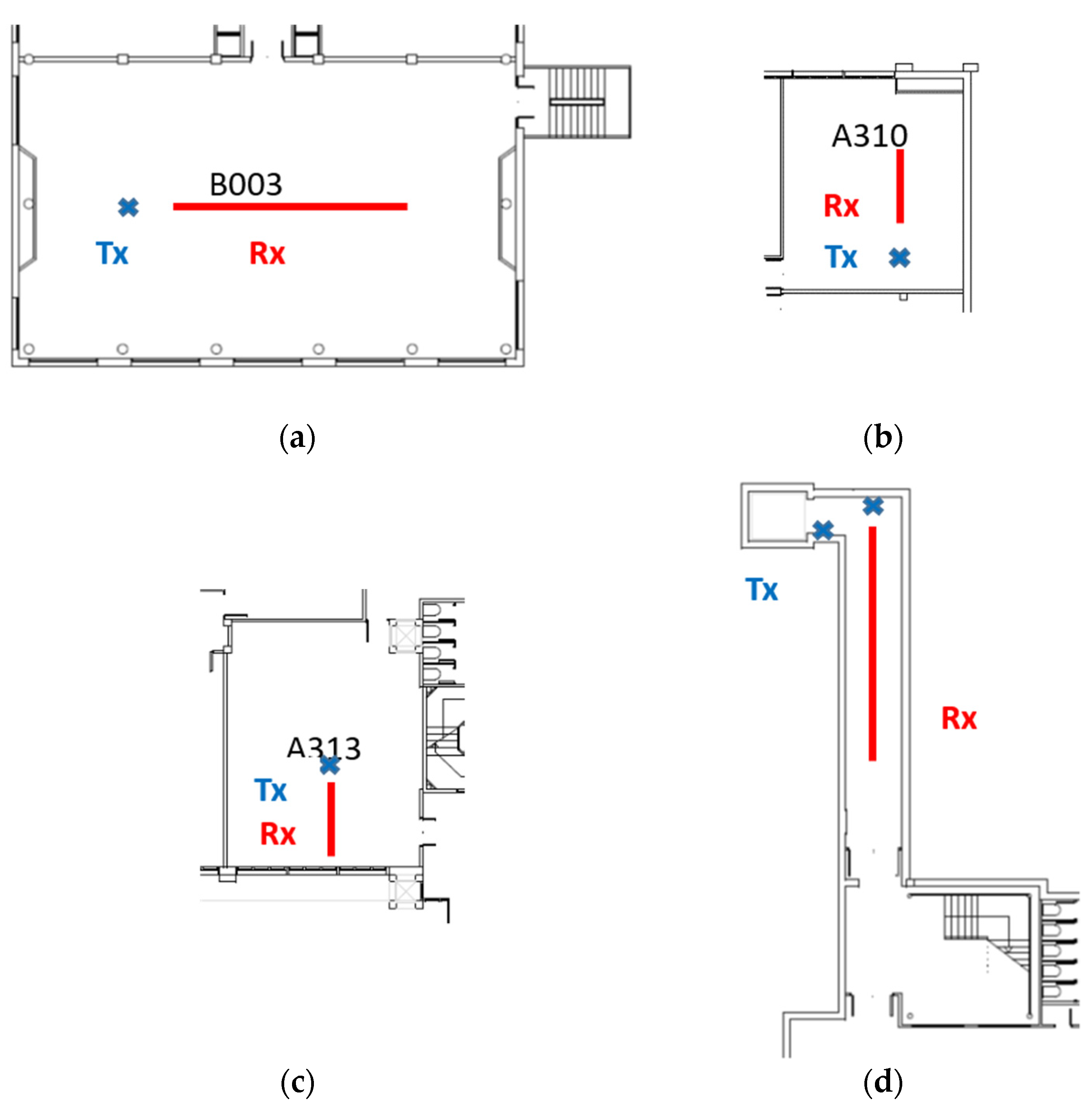
For 3 GHz band campaign, six scenarios were considered during the campaign: an auditorium, a corridor in both line of sight (LoS) and non-line of sight (NLoS) conditions, and two small labs, one of them full of furniture and stuff (labelled as Small lab #1) and the other (Small lab #2) in two configurations: empty and furnished.

The auditorium (B003) is a large classroom sizing 2030 cm long and 1230 cm wide. The receiver was moving along an 880 cm path, going further away from the transmitter, both being in the longest axis of the room. All the time, the LoS between the transmitter and the receiver is kept. The corridor is an underground tunnel 1452 cm long and 224 cm wide. The receiver followed a path along the axis for 880 cm, whereas the transmitter was aligned with it in LoS configuration, and shadowed by a corner in the NLoS. The small lab #1 (A310) is an 865 cm × 715 cm room, where the receiver was moving in parallel to the longest wall, all the time rounded by a lot of furniture, equipment, boxes and objects placed in a not well-organized manner. The small lab #2 (A313) is a rectangular room with dimensions 396 cm long and 635 cm wide. The receiver was moving along a path in the middle, parallel to the shortest wall. Measurements in the second small lab were made in empty and furnished conditions. Figure 2 depicts the maps of the four environments where 3 GHz data was gathered, all of them designed at the same scale.

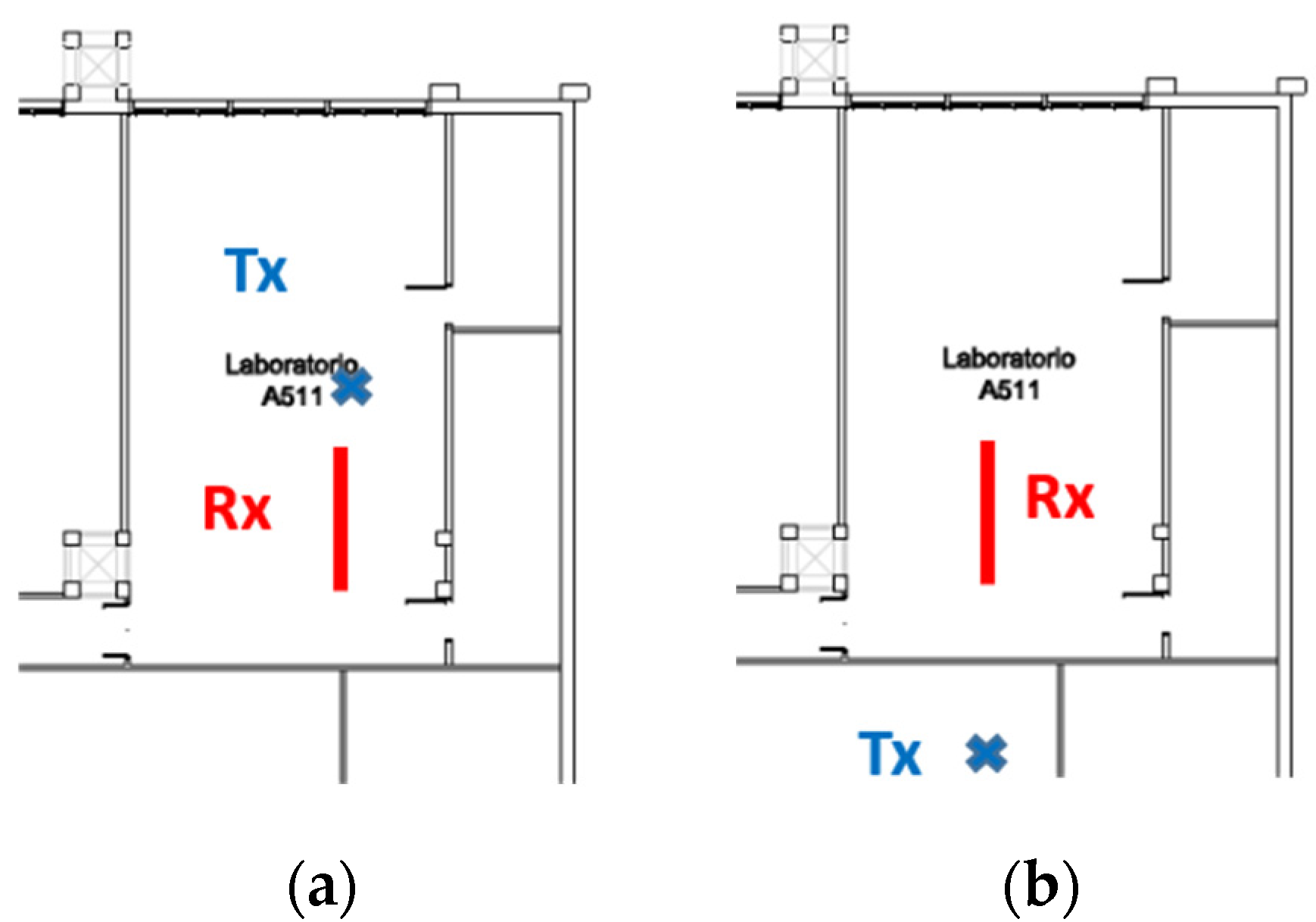
For the 5 GHz band campaign, up to five different scenarios were tested. A large lab (A510) hosted campaigns in both LoS and NLoS conditions. A medium size office was tested empty and furnished, in order to check the effects of furniture. Finally, a small lab, labelled as #3 (A514), was measured in LoS conditions to have data for comparisons with the bigger one as a function of the size of the room.

The largest lab size was 1100 cm × 700 cm. It is furnished with typical equipment of electromagnetic research labs: benches, stools, tables, chairs, cabinets, as well as equipment as analyzers or computers. Two series of measurements were gathered at this environment, one in LoS conditions and the other in NLoS. The office is 1200 cm long and 300 cm wide, and it was measured completely empty and then furnished with tables, chairs and computers around the receiving path, in a condition that could be considered OLoS. The medium lab is 750 cm × 700 cm and it was furnished as the large one. The maps and the location of transmitter and receivers along the measurement campaigns at each of the environments are in Figure 3, with all maps at the same scale.

2.3. Data Processing

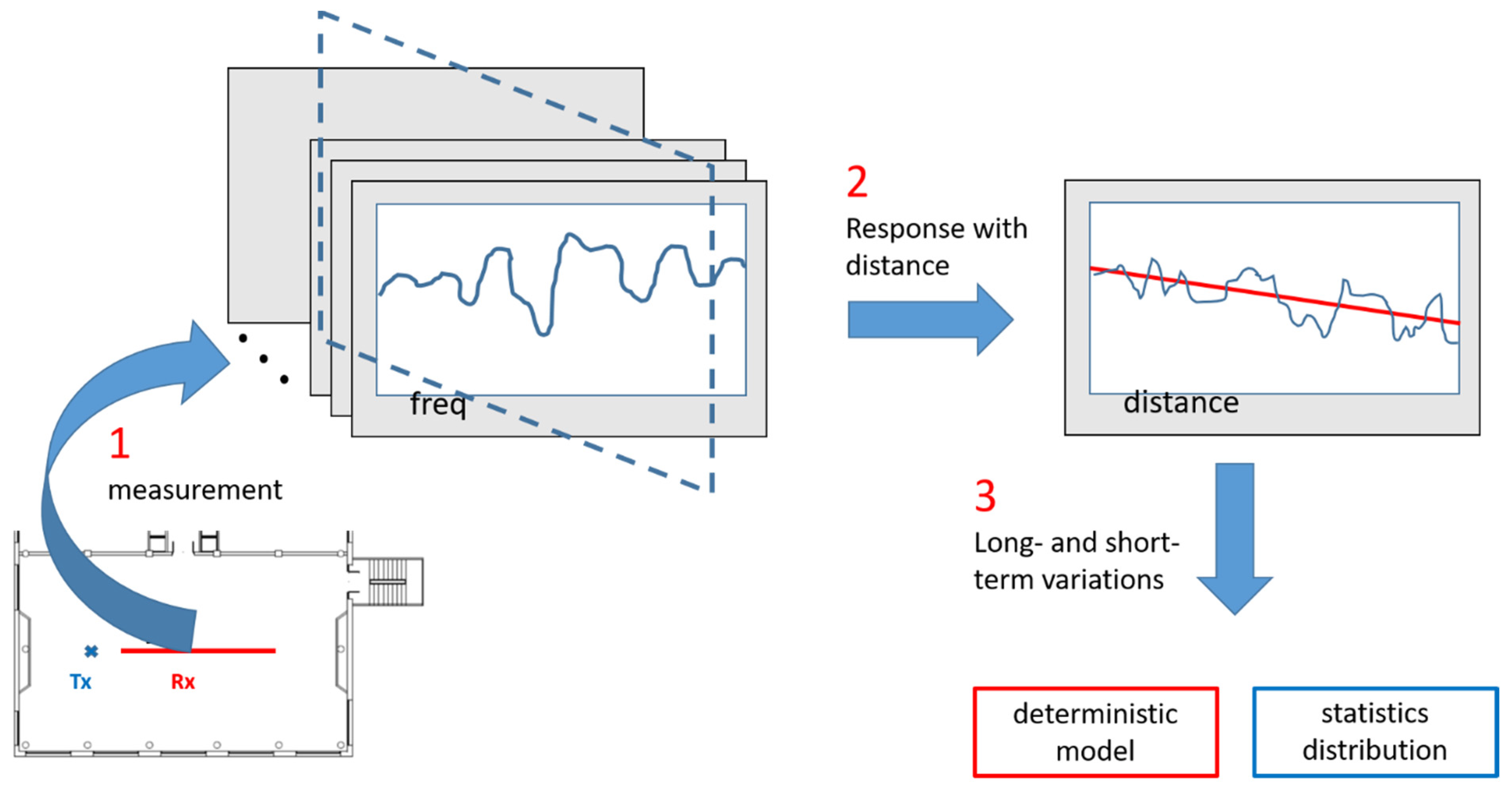
As a result of the measurement campaign, we have a collection of frequency responses, i.e., the description on the behavior of the radio channel in a number of frequency spots within a band, gathered at each measurement point. In fact, each of these frequency responses has 1001 frequency samples in the 3 GHz band measurements, and 801 samples in the 5.8 GHz band. As we measured at several points along a straight line path, with one eighth of wavelength separation, we can analyze the data as the response along space by selecting the values at a fixed frequency from each frequency response. Changing the point of view this way, what we have is a collection of channel responses along a linear path at different frequencies (in fact, at 1001 frequencies around 3.5 GHz and at 801 frequencies around 5.8 GHz). This kind of data is what we use to extract both long-term and short-term effects on the narrowband results. Figure 4 graphically depicts this process. Along the work, we are going to analyze the results at the center frequencies as the main target, although some additional information on the performance of the other frequency series will be also given.

When dealing with a mobile communication problem, the first element to consider is the losses due to basic propagation between transmitter and receiver, what is known as path loss. Following the recommendations ITU-R P.1238-11 [21], the path loss within a building and on the same floor can be defined with the following deterministic model:

PL = P_tx − P_rx = PL₀ − 10 n log₁₀(d/d₀) [dBm],

(1)

where:

• PL₀: Path Loss at a reference distance (d₀) [dBm].
• n: path loss exponent, indicating the rhythm of decay.
• d: distance between transmitter and receiver [m].
• d₀ reference distance (for simplicity it is usually 1 m) [m].

This path loss rule defines the slow or large-scale variations. Over those slow variations of the channel response, which are essentially deterministic, fast or small-scale variations associated with random, or difficult to predict, effects are observed. Once the deterministic losses of the channel are computed and removed from the channel response, the rest of the channel behavior should be explained by studying the random variations.

Since electromagnetic signals propagate through complex environments with obstacles and living beings or objects that move completely independently, the radio waves find multiple paths to travel between emitter and receiver. This type of multipath propagation implies that the power detected by the receiver is the sum of a multitude of copies of the same signal, but each with a completely different and random delay and attenuation. It turned out to be impossible to adjust this behavior to a deterministic model; so the alternative is to evaluate which probability distribution function is capable of predicting these variations introduced by the channel with greater accuracy. There is a wide variety of statistical models that can be used to adjust fast fading. First of all, recommendation ITU-R P.1057-6 [22] lists some of the most common probability distributions used with propagation prediction models. On the other hand, we must also take into account the results of previous works in which similar scenarios are analyzed [23,24], and take into consideration the models that have obtained positive results.

The adjustment of the fast variations with respect to these distributions is based on the maximization of the likelihood function. This procedure consists of finding the parameters of the distribution that maximize the probability that a given data set comes from said distribution [25]. Thus, the distribution that best fits will be the one with the highest probability. Commonly, this probability value is expressed in logarithmic units, so the criterion will be to choose the distribution that achieves the value of the highest log-likelihood.

As it is a numerical adjustment, the calculation error that may be made when carrying out the operations must be taken into account. Derived from the log-likelihood criterion [26], the Akaike’s Information Criteria (AIC) and the Bayesian Information Criteria (BIC) indexes support the decision of the statistical model that best fits the measured data.

AIC = −2 ln(L) + 2 k

(2)

BIC = −2 ln(L) + k ln(w)

(3)

where:

• L is the value of log-likelihood,
• w is the size of the sample,
• k is the number of parameters estimated in the model.

In both cases, the best model will be the one with a lower value. Although BIC penalties for additional parameters more than AIC, BIC is consistent, whereas AIC is not. Thus, in this work, we use BIC to determine the goodness of fit of the analyzed statistical models and, then, to decide which among them are the best for modeling the fast variations of the radio channel.

Once the BIC indexes are computed, it is possible to calculate ΔBIC: the difference between the best model (which presents the lowest BIC value) and any other among the considered models. ΔBIC can be used as an argument to support how good the best fitted model is. When ΔBIC is less than 2, the support provided by BIC index is barely worth a mention: it is not clear which really better fits the data, and the evidence is not statistically significant. When ΔBIC is between 2 and 6, the evidence is positive and the best model is well supported. For ΔBIC between 6 and 10, strong evidence supports the model decision; and when it is greater than 10, it is very strong [27,28,29].

3. Results

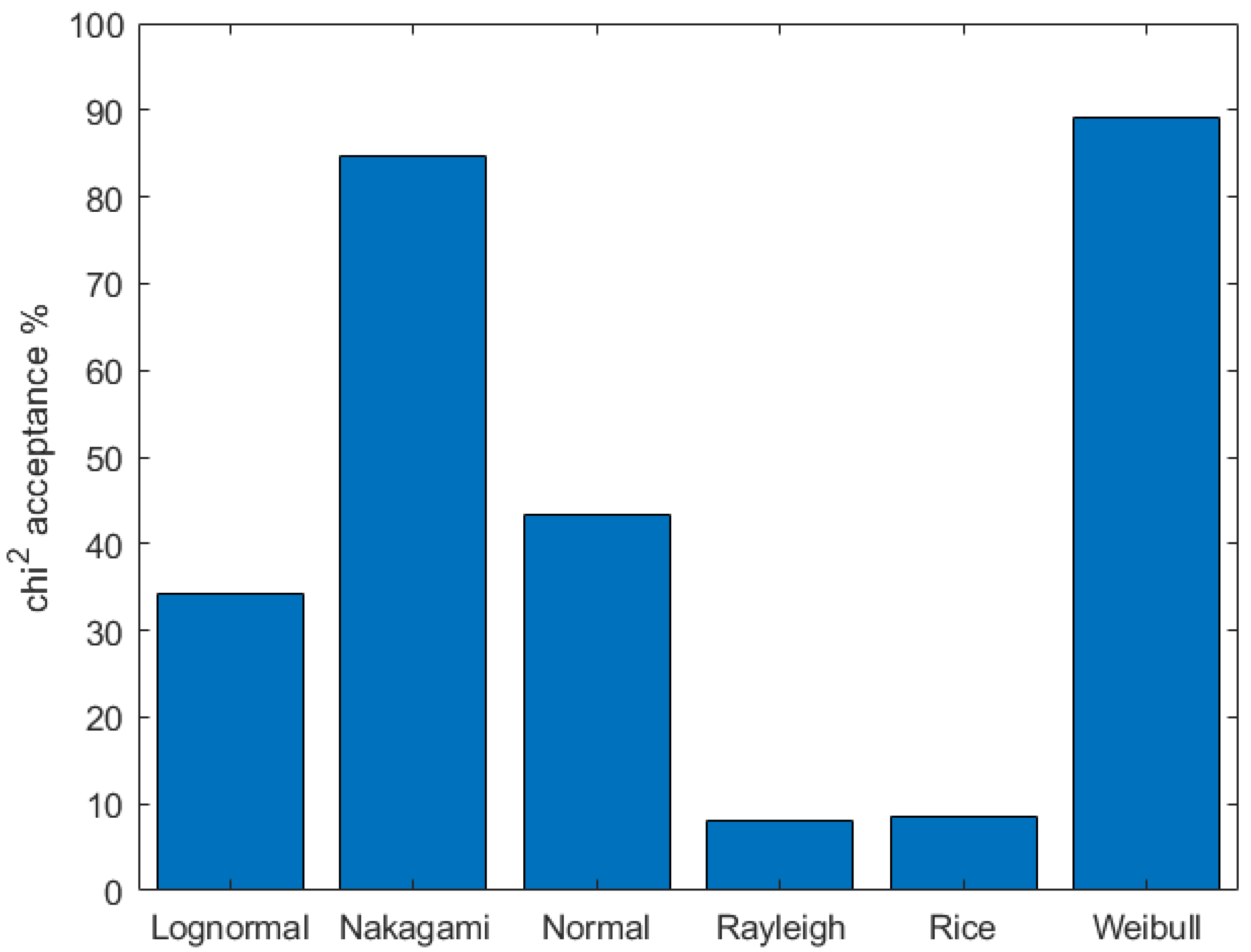
The presentation of the results is organized by frequency bands, along this section: firstly, 3 GHz band and, then, 5 GHz. In order to simplify the computational load and the analysis of the results, a brief pre-assessment is made to find which distributions may be relevant in this specific case. Using Pearson’s goodness-of-fit χ² test, the models that have >5% acceptance among all the data vectors of all environments resulted to be, in alphabetical order:

• Log-Normal.
• Nakagami.
• Normal.
• Rayleigh.
• Rice.
• Weibull.

Figure 5 summarizes this pre-assessment, comparing the performance of the best fitting distributions at all the measured frequencies and at all the environments. This chart indicates that Weibull and Nakagami distributions seem to provide the best results when fitting the fast fading data at all considered environments and frequencies.

3.1. Results at 3 GHz Band

Broadband analysis of the complex frequency responses at 3 GHz band is the content of [30]. As indicated in Section 2.3, considering the values gathered at different measurement points along the straight paths at fixed frequency samples, a series of narrowband data is available for analyzing the narrowband behavior, and among other effects, their fast variations. Slow variations are defined by the exponent of the path loss model, and once these large-scale effects are removed from the results at the different environments, the data are ready for the statistical analysis of the short-scale or fast variations. Once checked up to six distributions, those previously selected as providing less fitting error, Weibull and Nakagami distributions performed better than all the others. Using this pair of distributions, we can compare all the environments under study, as initially done at

Table 1. ΔBIC values at different measurement environments, at 3.5 GHz response.

Environment	Visibility Conditions	Distribution
		Normal	Rayleigh	Weibull	Rice	Nakagami	Lognormal
Corridor	LoS	192	279	19	285	BIC*	163
	NLoS	338	535	BIC*	540	20	53
Auditorium	LoS	312	365	BIC*	371	31	52
Small lab #1	OLoS	113	153	3	158	BIC*	73
Small lab #2	Furnished	103	150	BIC*	154	7	11
	Empty	49	57	BIC*	61	BIC*	24

with the ΔBIC values for the 3.5 GHz response, corresponding to the central frequency of the measured band. The best performing distribution is identified as BIC* in each environment. In all situations, the BIC* model provided strong evidences to support its selection.

Observing Table 1, Weibull distribution appears to be the best choice for 3.5 GHz in most of the environments, being the others governed by a Nakagami formula. The other four models can be clearly rule out considering the values for ΔBIC. It is worth mentioning that Weibull selection is in accordance with studies conducted at the 2.4 GHz band [5,14], which could be considered a support for these results, as the frequency bands are not so separated.

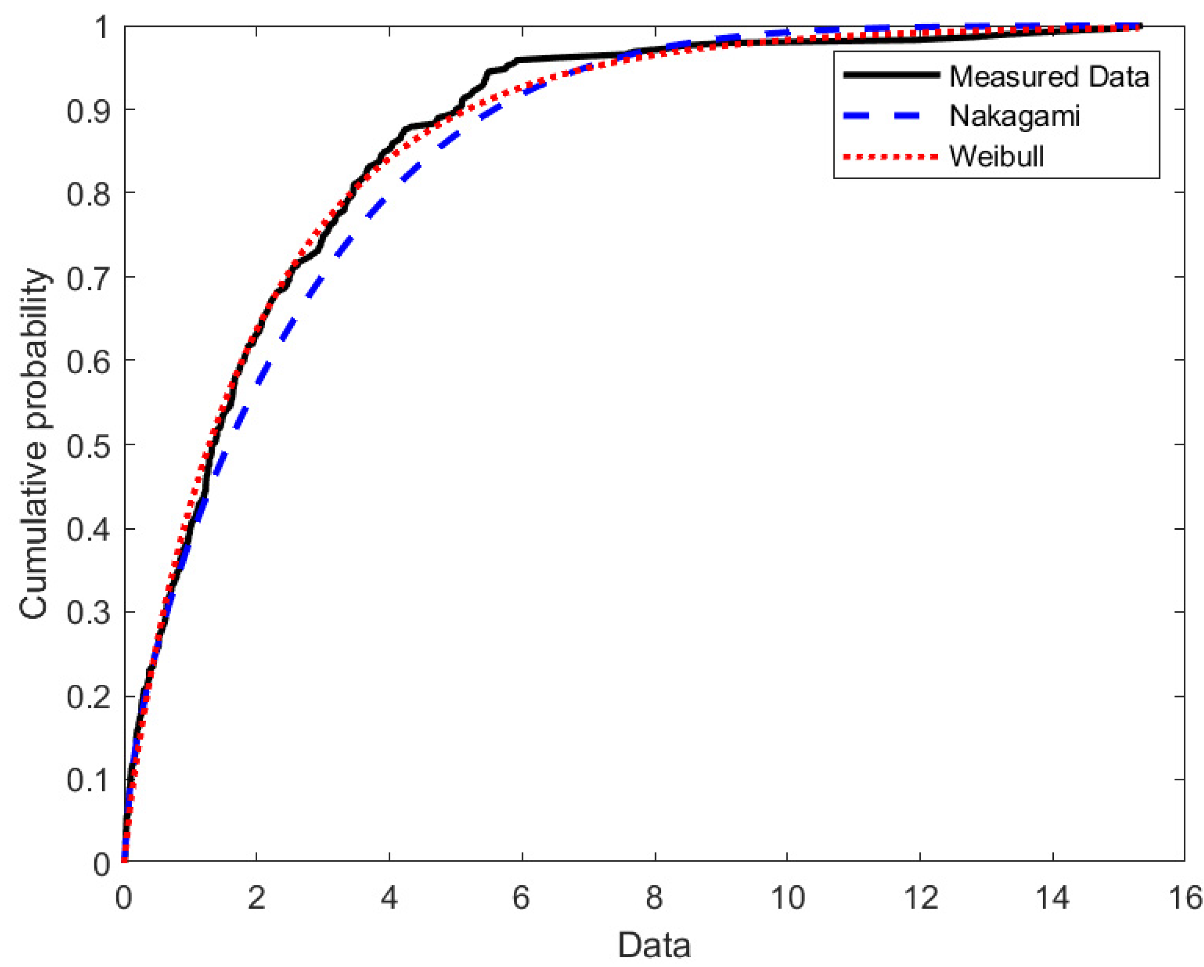
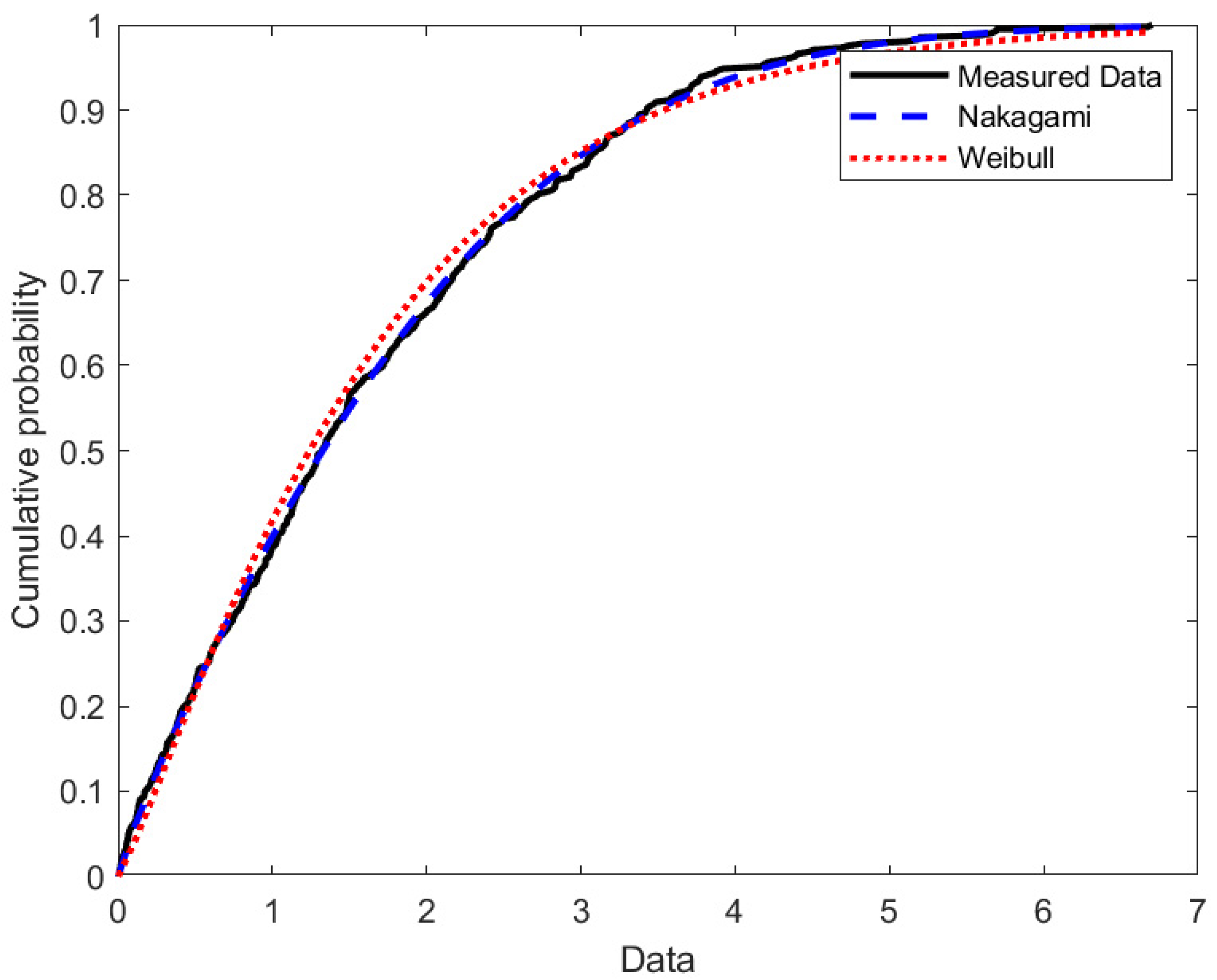
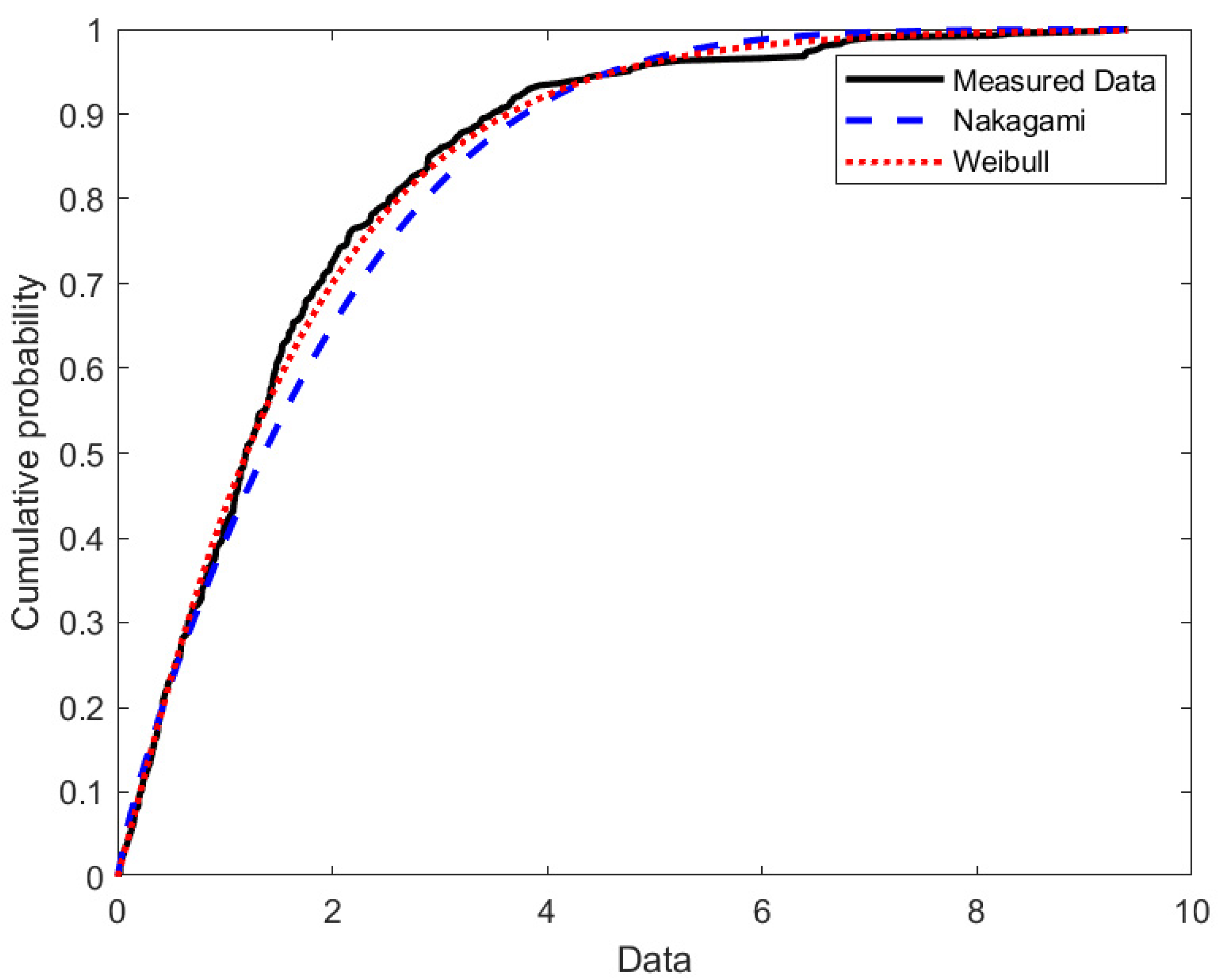
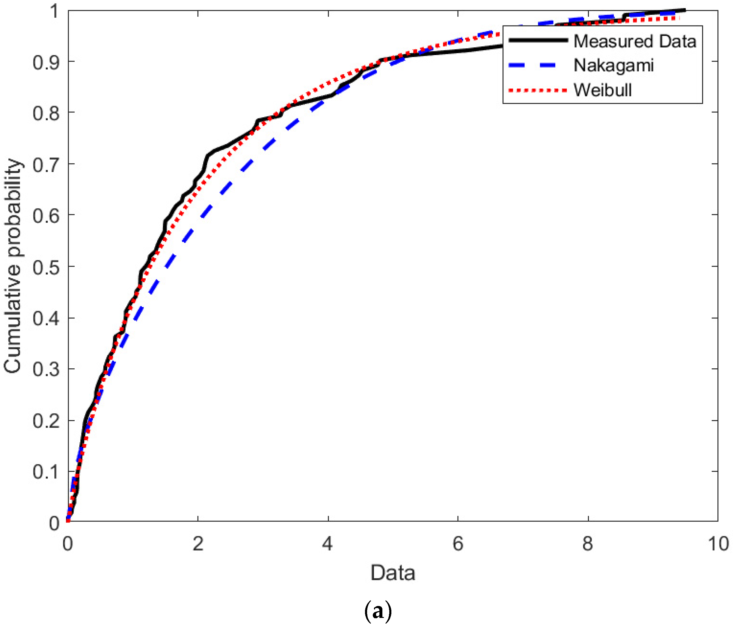
Figure 6 shows the fittings provided by Weibull and Nakagami distributions regarding corridor LoS data, in terms of cumulative distribution probability (CDF). Visually, Nakagami seems to fit better than Weibull, although both distributions perform in a good way. Then, ΔBIC numerical analysis at Table 1, regarding 3.5 GHz frequency spot, is confirmed by the observation of Figure 6.

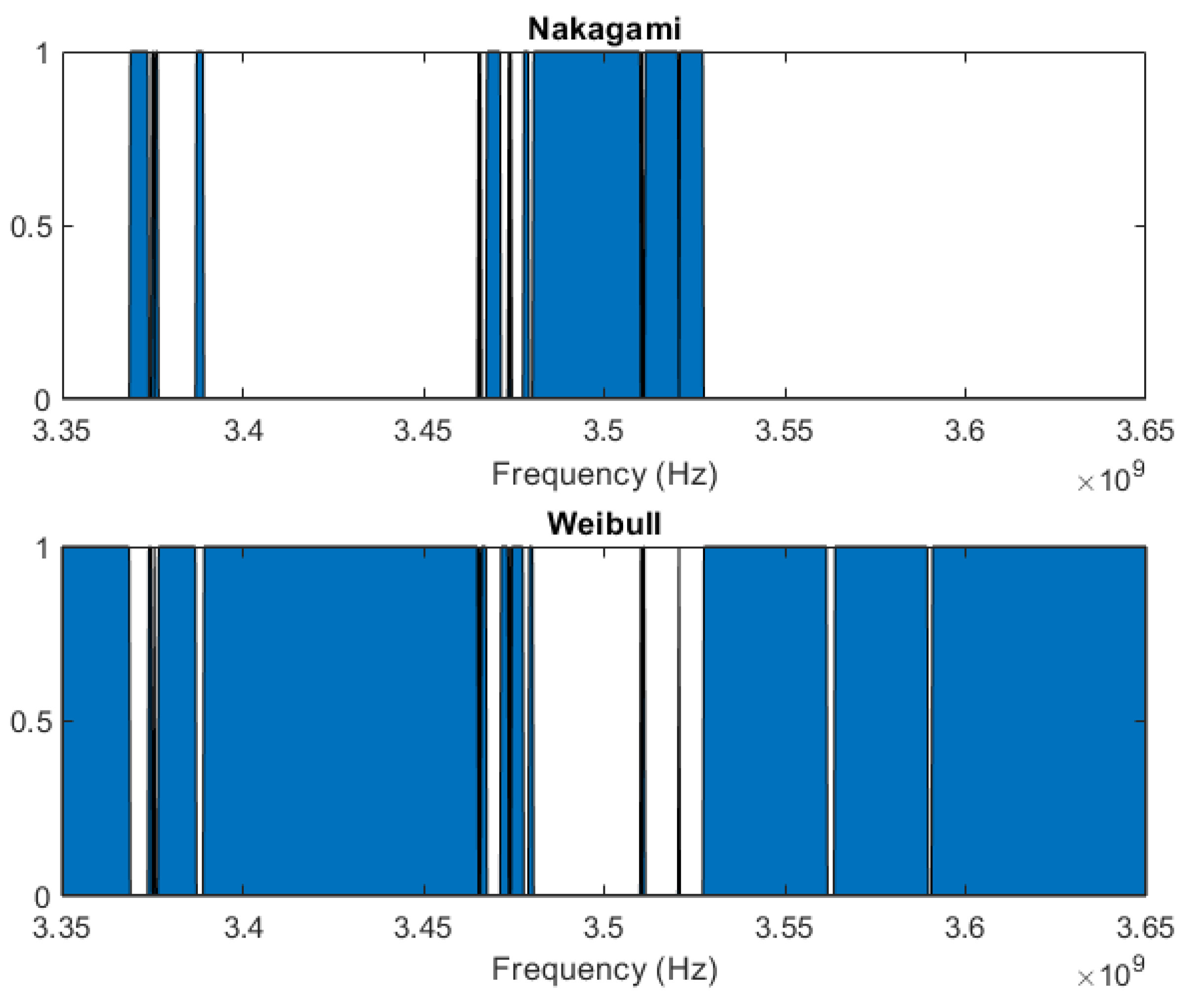
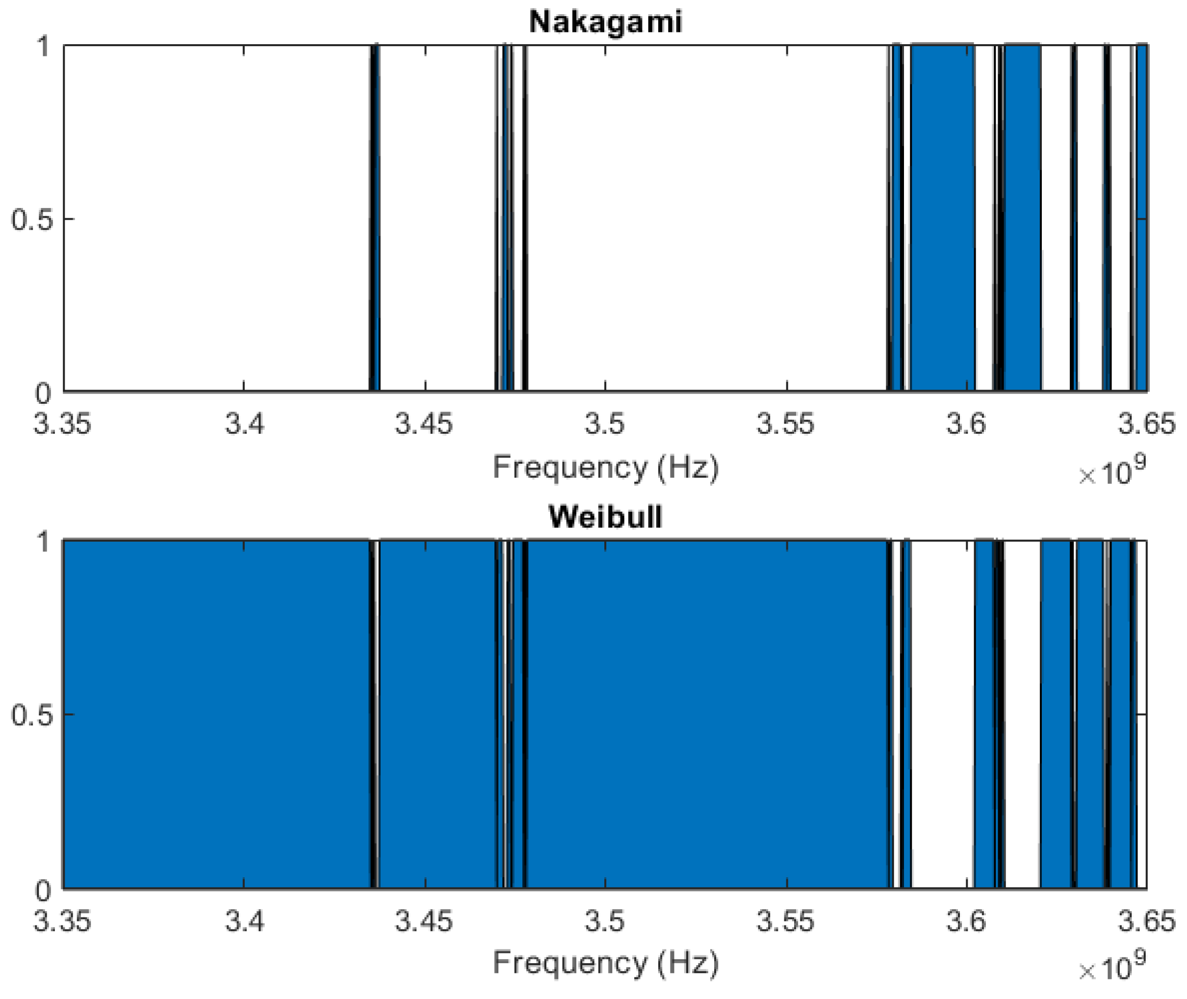
Completing the information provided by Figure 6, Figure 7 depicts the different best fittings along the complete frequency band in the corridor, in LoS conditions. It could be observed that although Nakagami fits better at central frequencies (as 3.5 GHz, being congruent with Table 1 results), Weibull does at many other sections of the considered spectrum section. In fact, we can observe that there are more frequencies at which the channel short term responses follow Weibull than those following Nakagami distributions.

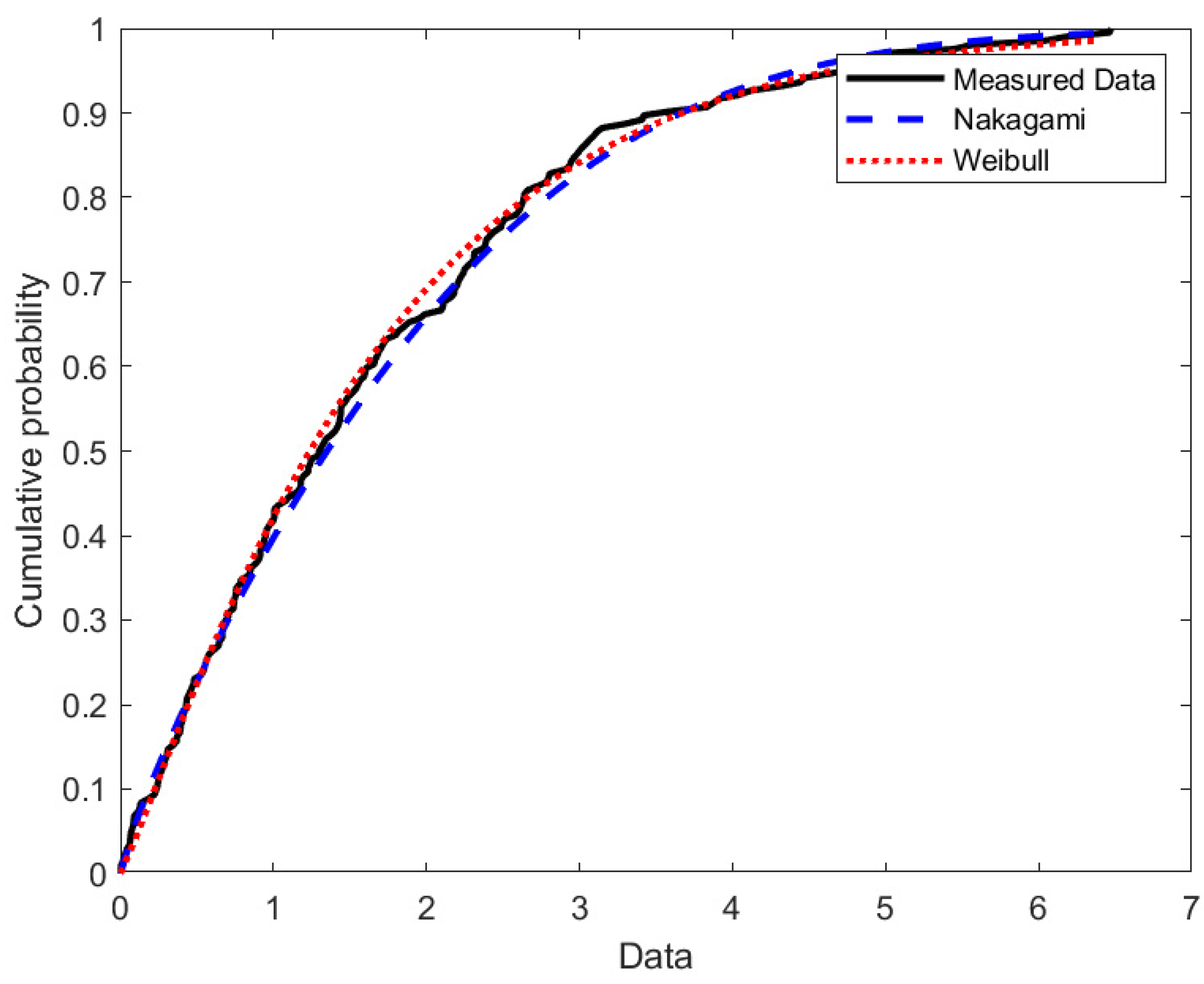
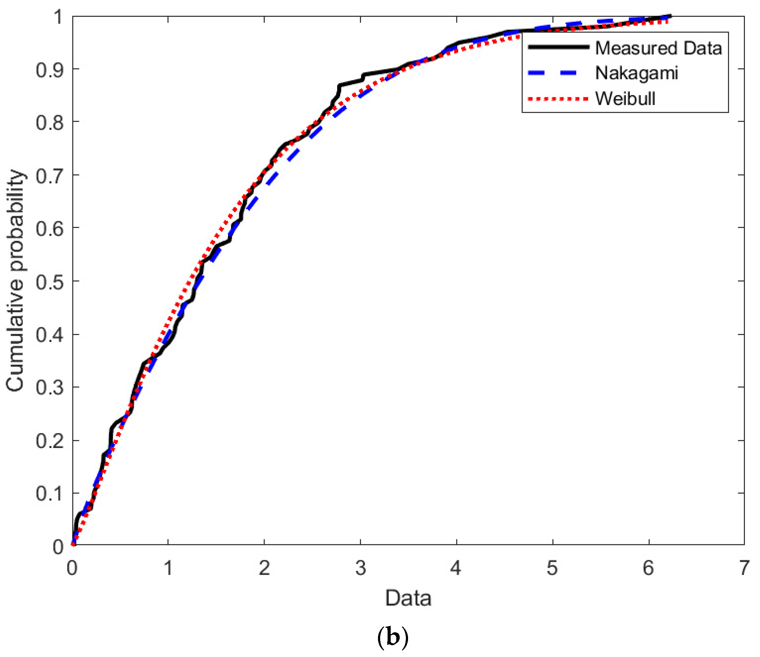
Figure 8 shows results for the same corridor of Figure 6, but for the case of NLoS conditions. In this situation, it is Weibull distribution that seems to perform better than Nakagami at the frequency spot 3.5 GHz, and data at Table 1 confirms this visual conclusion. Besides, Figure 9 allows us to check that Weibull fits better in most of the 1001 frequency lines analyzed within the 3 GHz band.

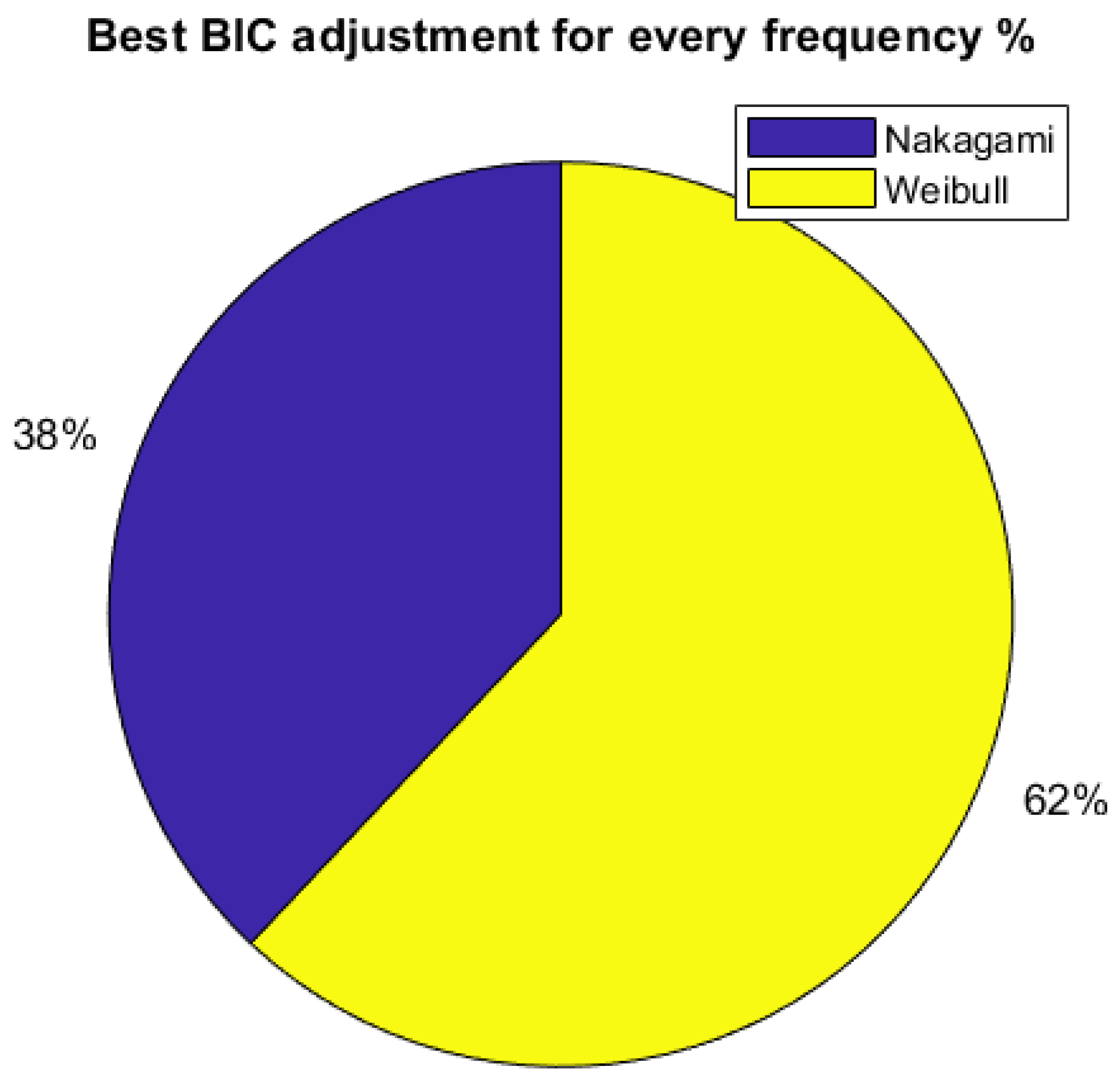
Analyzing the results obtained at the auditorium (see Figure 10), Weibull again performs better than Nakagami, confirming the prediction of ΔBIC analysis in Table 1. In fact, the differences in fitting goodness seem to be larger than in the case of the corridor, which is reflected in the different ΔBIC values: in the corridor NLoS, ΔBIC is 20 when comparing Nakagami to Weibull (the best fitting distribution); and in the auditorium, this ΔBIC is 31.

Figure 11 indicates the percentage of frequency lines best fitted by each of the considered distributions in the auditorium, providing similar information than Figure 7 or Figure 9 for the corridor. In 62% of the 1001 frequencies included in the studio, Weibull distribution is the best-performing among those considered; and in the other 38%, it is Nakagami. The other statistical distributions are not the best for any frequency line in the auditorium channel responses.

Figure 12 contains the comparison between Weibull and Nakagami when fitting the fast variations gathered within the small lab #1. Visually, it is not easy to decide which of these distributions performs better. Additionally, numerically, using the ΔBIC values, it is possible because Weibull is three points worse in the Bayesian test. In this case, we can say that ΔBIC analysis allows us to take a decision that was impossible only by direct inspection.

Finally, the comparison of fitting using Weibull and Nakagami models for small lab #2 in both empty and furnished configurations are depicted in Figure 13. In both cases, Weibull performs graphically well, confirming the insight provided by ΔBIC analysis.

In general terms, the results obtained at 3 GHz band indicate that ΔBIC analysis appears to be a good indicator for a fast decision on the statistical distributions to be used to model the fast variations on the channel response. What is suggested by this numerical exploration coincides with the subjective decision that a researcher could provide when observing the CDF plots of the different fittings, and it is also useful in cases with difficult decisions by direct inspection.

As a summary of this section,

Table 2. Values for the different parameters of statistical distributions at 3 GHz band.

Environment	Visibility Conditions	Distribution
		Weibull		Nakagami
		Scale (a)	Shape (b)	Shape (µ)	Scale (Ω)
Corridor	LoS	1.7317	1.1280	0.4287	4.5627
	NLoS	1.9761	0.8586	0.2930	10.6208
Auditorium	LoS	1.6840	1.0833	0.4027	5.1147
Small lab #1	OLoS	1.7352	1.0981	0.4128	4.8834
Small lab #2	Furnished	1.7027	1.0514	0.3880	5.4965
	Empty	1.7172	1.0275	0.3757	5.8678

contains the parameters governing Weibull and Nakagami distributions that better fit the measured short-term variations at 3 GHz band. Both distributions resulted as the best performer among the six considered in this band.

We can observe that the scale parameter of Weibull distribution seems to be generally lager when the line of sight is cut: this occurs in the corridor, or comparing the results of small labs #2 in empty conditions and #1 in OLoS. Additionally, in smaller rooms, this scale Weibull parameter is larger than in larger rooms (comparing small labs and auditorium). Nakagami parameters seem not to follow a clear trend regarding the visibility or the room size.

3.2. Results at 5 GHz Band

Measurement outcomes consisted of five collections of complex frequency responses, which broad band performance has been described in [31,32]. From these data, five series (one for each of the environments) of 801 vectors of narrowband data (one for each of the frequency spots) give us information on the narrowband behavior of the channels. They are analyzed as explained in Section 2.3, beginning by separating the slow to the fast variations. Slow variations are modeled following the exponentially decay path loss model. Once modelling the slow variations, the fast variations are all measured data not explained by the path loss model. These are the data then modeled by different statistic functions. As in the previous frequency band, the results from different environments at 5 GHz band are analyzed in terms of ΔBIC values, and summarized in

Table 3. ΔBIC values at different measurement environments, 5.8 GHz response.

Environment	Visibility Conditions	Distribution
		Normal	Rayleigh	Weibull	Rice	Nakagami
Large lab	LoS	4	107	3	BIC*	14
	NLoS	33	17	BIC*	1	1
Office	Furnished	28	19	BIC*	1	1
	Empty	26	18	2	BIC*	3
Small lab #3	LoS	8	66	1	BIC*	6

. The best performing distribution is identified as BIC*. Taking into account these results, Rice distribution appears to be the most convenient for modelling fast variations in the LoS large lab, whereas in NLoS conditions, Weibull is the best approach. Anyway, differences between BIC values for each distribution compared to BIC* resulted to be lower than in the 3 GHz band, and in some cases they are not so significant. As a general comment, it seems that Rice performs better in LoS conditions and Weibull in NLoS or in obstructed LoS, but this comment is limited by the not so strong significance of some decisions. In fact, considering the significance of the analyses, again Weibull and Nakagami would provide the best results in most of the conditions (4 over 5, actually), as those with ΔBIC equal of below 2 are not possible to support by this numerical study.

Some publications, such as [17,18,19], studied more complex distributions that combine Rayleig, Rice, Nakagami and others to model indoor millimeter wave bands, as those correspond to the FR2 spectrum for 5G. The results at 5.8 GHz, which is a FR1 band closer to FR2 than 3 GHz, seems to connect with these proposals that combine some of the analyzed distributions, as some of them provide really similar fitting performance within the same measured data.

Figure 14 and Figure 15 compare the fitting of the better distributions for the largest environment in LoS and NLoS conditions, respectively. As expected by the very small ΔBIC value comparing the “second classified” model to the best fitting, it is really difficult to decide for the best choice just by visual inspection of both CDF plots.

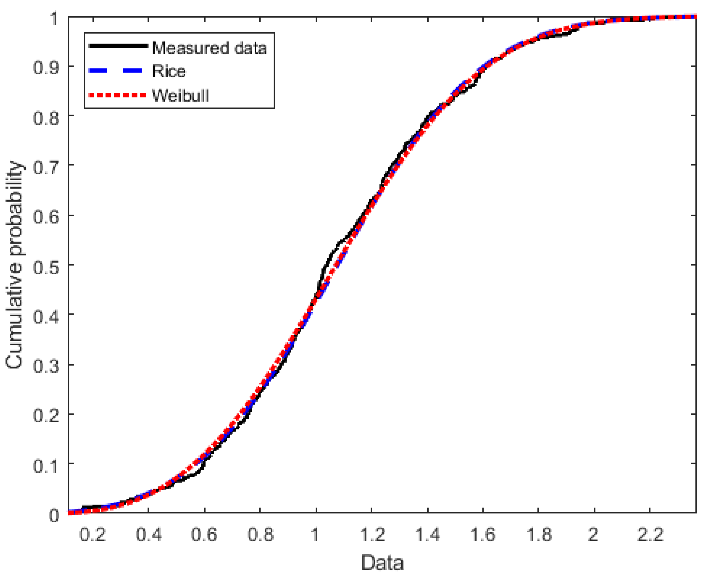
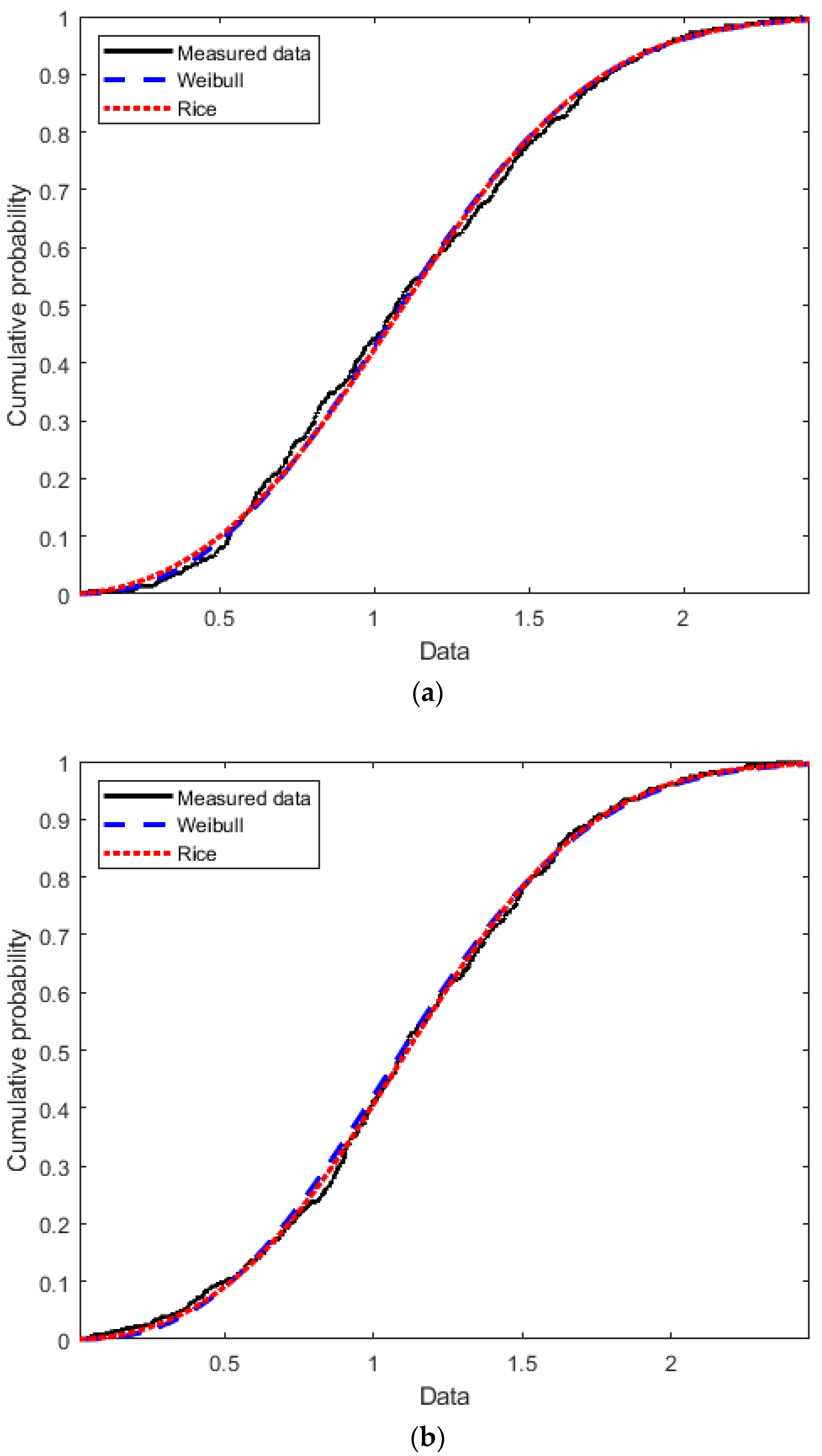
Comparing the empty and furnished office, the results are consistent with the previously commented situation: in conditions with LoS, as it is the case of the empty room, Rice obtains the better results, although ΔBIC analysis does not allow a clear decision comparing to Weibull model: observing Figure 16a, it is really difficult to select the best fitting considering both plots. Once the room is furnished, and then the LoS is partially obstructed, Weibull is the distribution performing better than Rice, but again, ΔBIC values are very low, and the graphical representation at Figure 16b shows a comparison between two very similar fittings.

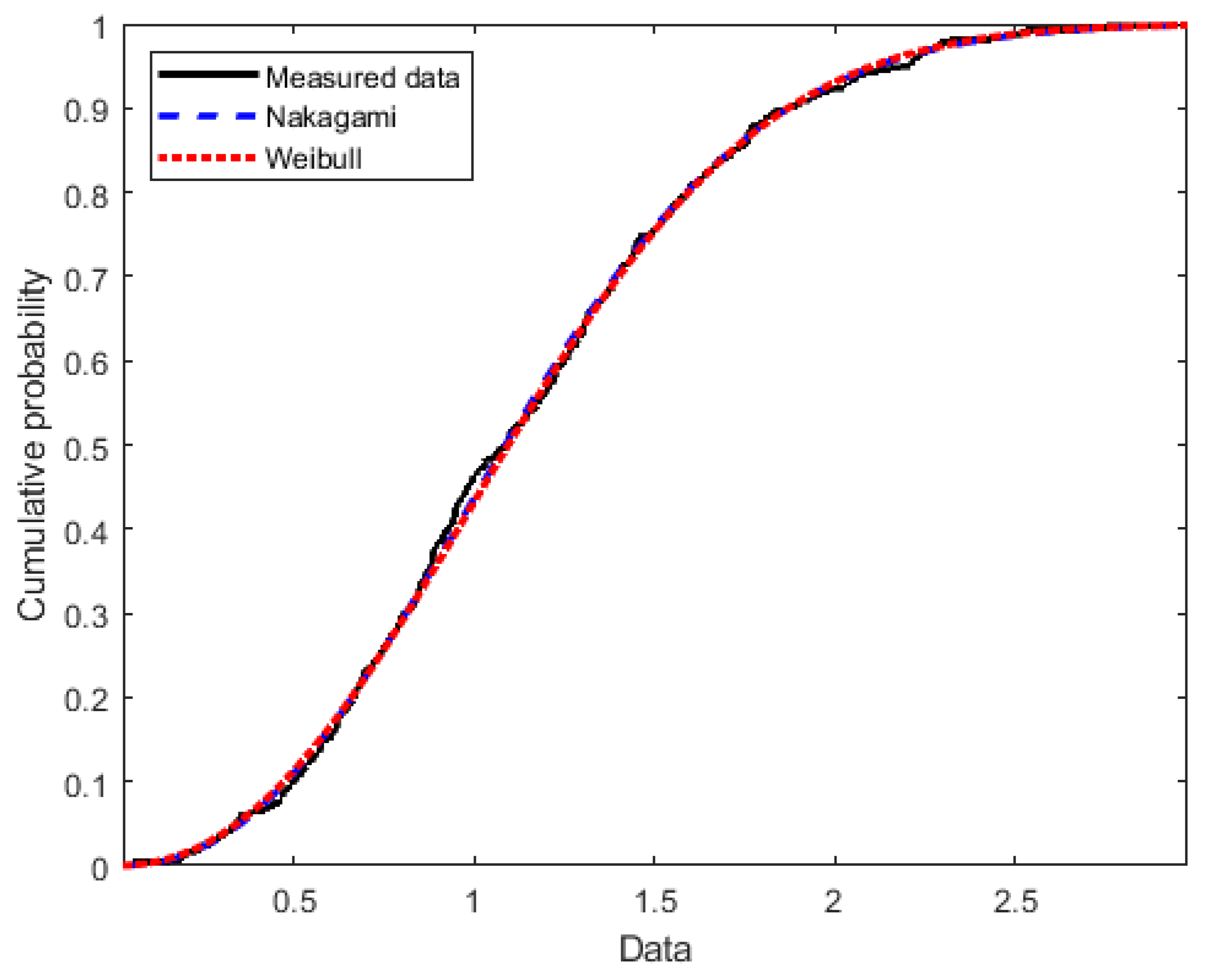
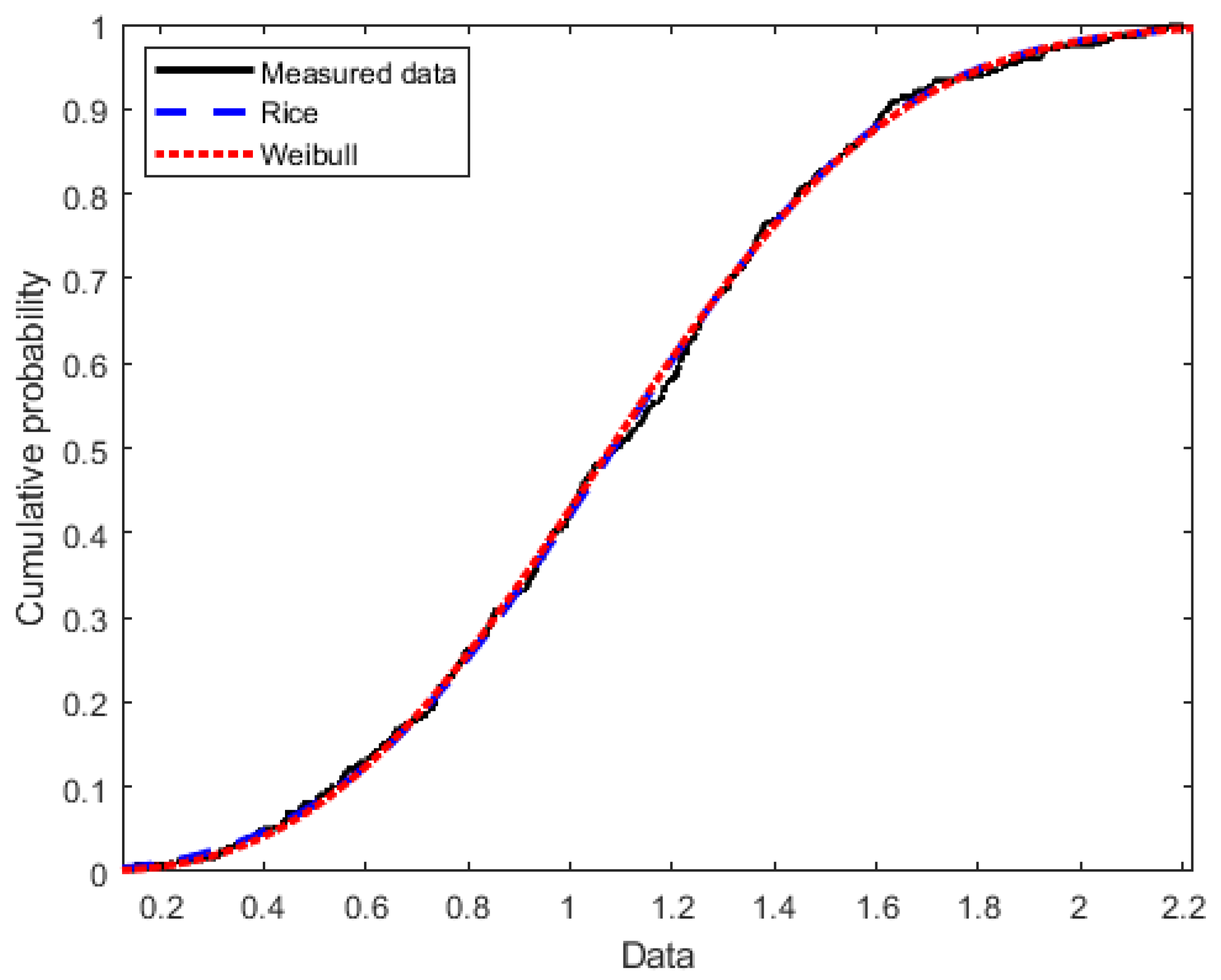
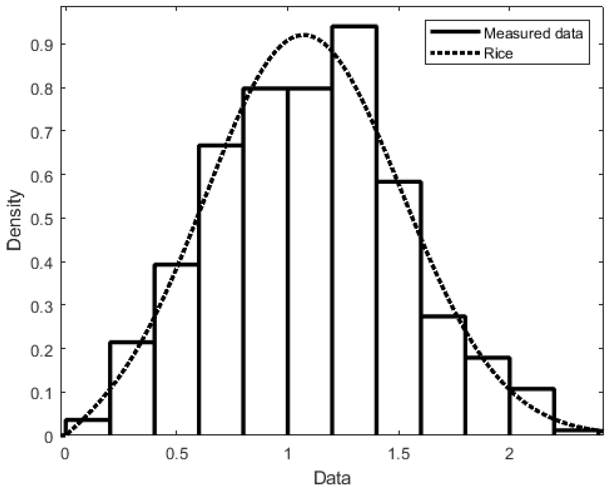
Results in LoS conditions at the small lab #3 indicate that Rice and Weibull models perform very similarly in both numerical terms (ΔBIC) and subjective terms (direct inspection), as observed in Figure 17. The Rice adjustment is also indicated in terms of histograms for this case, as an example of the statistical distributions fitting, in Figure 18.

Table 4. Values for the different parameters of statistical distributions at 5 GHz band.

Environment	Visibility Conditions	Distribution
		Weibull		Rice
		Scale (a)	Shape (b)	Distance (ν)	Scale (σ)
Large lab	LoS	1.1820	3.4461	1.0005	0.3509
	NLoS	1.2323	2.7783	0.9766	0.4652
Corridor	Furnished	1.2328	2.7367	0.9705	0.4728
	Empty	1.2376	2.6863	0.9641	0.4870
Small lab #3	LoS	1.2030	3.2252	0.9953	0.3929

contains the values of the parameters of Weibull and Rice distributions that provide the best fitting among all the considered in the 5 GHz band. In the Rice column, “distance” refers to the distance between the reference point and the center of the bivariate distribution.

As observed at 3 GHz, the scale Weibull parameter at 5 GHz increases when passing from LoS to NLoS conditions. Besides, in smaller rooms (small lab #3), this parameter seems to be larger than in larger rooms (large lab), following again the same trend that in 3 GHz band. The distance Rice parameter follows the inverse trend: it decreases when changing LoS by NLoS conditions, and it increases when the size of the room is smaller.

4. Discussion

The proposed use of ΔBIC for deciding the best performing statistical model for fast variations seems to work appropriately. In fact, the results given by this analysis are in the line of the observations provided by direct inspection: when ΔBIC indicates a clear best fit, this is also observable at the graphic results; and when ΔBIC gives inconclusive support, plots look more or less the same.

Regarding the 3 GHz band analysis, Weibull model performs better than the others within all environments at 3.5 GHz frequency line, except the corridor in LoS conditions, where Nakagami is the best (although Weibull wins in most of the other frequencies within the band). This environment is a bit different than the other indoor scenarios, where the LoS were cut or obstructed, or at least there were some elements (furniture, equipment) within the first Fresnel ellipsoids at the radio link between transmitter and receiver. The corridor was completely empty, and the receiver path was placed exactly along the axis of the room, which increases the possibility of something like a tunnel effect due to the symmetry.

The presence of furniture in the small lab #2 increases the advantage, in terms of BIC, between Weibull and Nakagami models: when the environment is furnished, ΔBIC is 22, whereas in the empty room it was only 6. This reinforces the previous comment: the fast variations follow a distribution more Weibull when there are more elements within the environment, perhaps some of them even within the first Fresnel ellipsoid, and it is more Nakagami when the environment is free of any kind of obstacles or objects.

In bigger rooms, Nakagami resulted to be more disadvantaged regarding Weibull, presenting larger ΔBIC values.

Moving to 5 GHz band results, the analysis with ΔBIC resulted to be less conclusive than at 3 GHz. However, some remarks can be extracted. In general, Rice and Weibull models resulted to be the dominant within the five different environments considered, although Nakagami would also be valid for modeling some of the environments.

The obstructed LoS conditions, basically when a brick-wall separates transmitter and receiver (large lab, NLoS) or when furniture occupies the office (not blocking the LoS but invading the first Fresnel ellipsoid), Weibull is lightly over assessed in comparison with other alternatives, although Rice and Nakagami appear not to be disposable at all. In fact, visual inspection of CDF fittings does not allow us to decide which among the possible models looks better adjusted.

Rice is better marked in all LoS conditions, Weibull also being valid in most of them. Nevertheless, Nakagami appears to be inaccurate for such LoS environments, with ΔBIC values larger than 2.

In larger rooms, as in the 3 GHz bands, Nakagami performs poorer than in shorter places, being the ΔBIC value for the large lab clearly larger than for small lab #3.

5. Conclusions

This manuscript shows the analysis of the statistical behavior of short-term or fast variations within the radio channel response at indoor academic environments at two bands in the 5G FR1 spectrum: 3 GHz and 5 GHz. Besides the more typical analysis based on the fitting of CDF traces, deeper conclusions are extracted based on ΔBIC (difference on the Bayesian Information Criteria indexes computed with the best fitting model and any of the other analyzed). Graphical results are provided and compared to numerical, observing a good correspondence on the selection of the statistical models than best represent the observed phenomenon.

In the 3 GHz band, Weibull models performs better than the others, except in some specific frequency spots for which Nakagami results to be more adequate. In the 5 GHz band, most of the environments responses could be explained by Rice or Weibull indistinctly, as ΔBIC between both are inconclusive to determine the most suitable.

Independently of the frequency band, it seems that the size of the room has a clear impact: the larger the room, the larger the ΔBIC of Nakagami respected to the best fitted distribution. This means that Nakagami’s performance turns worse when the size of the room increases.

Regarding the Weibull distributions that provide the best fitting in different environments, it can be observed that the scale parameter increases when visibility conditions change from LoS to NLoS, and it is also larger in smaller rooms. This was observed at both considered frequencies.

The data provided about fast variations in the channel response, as well as the proposal of using ΔBIC for such analysis, should be useful for network planners during the tasks of designing a new deployment. Specifically, and considering the frequencies analyzed along this work, 5G development would be improved when network designers take into account the proposed models. Some of the current applications (i.e., indoor localization), as well as many upcoming proposals, could be affected by the fast fading events as signal level has capital importance in their developments. Having a more precise modeling is the first step to assure a good performance of these new services. In fact, the contents of this paper connect with and complement previous studies made at different frequencies, and its conclusions result to be coherent with those performed at lower and higher bands.