Simple, Fast, and Accurate Broadband Complex Permittivity Characterization Algorithm: Methodology and Experimental Validation from 140 GHz up to 220 GHz

Abstract

Accurate permittivity characterization has attracted a lot of attention in various areas. Resonant characterization methods are well-known for their accuracy, but they are restricted in very narrow frequency ranges, and thus, they are normally not recommended to be used for dispersive or high-loss materials. Transmission line characterization techniques are outstanding for being inexpensive, accurate, and broadband, but the algorithms are often complex to perform. This paper proposes a fast, simple, and accurate broadband permittivity characterization algorithm, which is mainly suitable for millimeter-wave applications. It combines a general line–line method and a closed-form algorithm, extracting the complex permittivity of the material under test (MUT) without the need for calculating any intermediate parameters. Validation measurements on de-ionized water in the frequency range from 140 to 220 GHz are in very good agreement with the literature data, which successfully indicates that the proposed algorithm is reliable and accurate for millimeter wave permittivity characterization.

1. Introduction

Accurate complex permittivity characterization has attracted a lot interest in various research fields and in enormous engineering applications [1,2]. For instance, with the development of 5G technology, the accurate characterization of substrate parameters, especially at millimeter and terahertz frequencies, is highly important [3,4,5]. Permittivity measurement is also playing an increasingly important role in agriculture, the food industry, material science, and biomedical engineering in the last few years [6,7,8,9], due to its obvious advantages of being direct, label-free, sensitive, nondestructive, etc. One emerging application is the real-time detection and characterization of chemical or biological liquids. This has been used for genetic analysis [10], determination of mixtures’ composition [11], thickness estimation [12], etc.

Generally, permittivity characterization techniques can be classified into resonant and non-resonant techniques. For the resonant methods, a resonant cavity [13,14,15] or a printed resonator [16,17,18,19] is usually designed, with the material under test (MUT) being located in the cavity or loaded on the sensing area. By analyzing the variations of the resonator’s resonant frequency and quality factor, one can extract the MUT’s complex permittivity. These resonance-based permittivity characterization techniques are highly sensitive, easy to perform, and normally inexpensive, but unfortunately, they can be only used for analysis within a narrow-frequency bandwidth. Moreover, in the resonance-based methods, the MUT’s complex permittivity is assumed to be constant within the narrow frequency range of interest. Thus, they are not suitable for characterizing dispersive materials, whose complex permittivity is highly frequency dependent. Furthermore, the resonant methods are not recommended for characterizing high-loss materials, since the sensitivity and accuracy can be appreciably compromised due to the dramatic decrease of quality factor.

Non-resonant techniques mainly rely on analyzing reflected and/or transmitted electromagnetic waves from the MUT, and they normally characterize materials within a broadband frequency range. The most widely used technique is the open-ended coaxial probe method [11,20,21]. By immersing the probe in liquid or powder MUTs, the complex permittivity can be extracted from the reflection coefficients. The open-ended method can provide permittivity results over a wide frequency range, but it is mainly used for low frequencies (normally <50 GHz). Moreover, as the open-ended probe method assumes the MUT to be semi-infinite, the measurement results are usually not accurate for low dielectric constant and low-loss materials. Another often used method is the free-space technique [22,23]. In this method, the MUT is positioned between two antennas and the MUT’s complex permittivity is extracted from the reflected and transmitted electromagnetic waves received by the antennas. The free-space method is contactless, but a special preparation procedure is often necessary.

The transmission line (TL) permittivity characterization techniques, being classified into the non-resonant group, have been developed for decades [24,25,26]. Typically, the MUT is located inside or on top of the TL [27,28,29,30]. The propagation constant and the characteristic impedance of the TL can be dramatically changed after loading the MUT. Therefore, by analyzing the variation of scattering (S-) parameters (including the transmitted and reflected coefficients), one can calculate the change of the propagation constant and the characteristic impedance and finally obtain the MUT’s complex permittivity within a broad frequency band. These techniques are highly accurate and can provide very broadband permittivity measurements. Furthermore, the TL methods are inexpensive and have no restriction on the shape, form, loss property, etc. of the material to be analyzed. In order to characterize bio-fluids at high frequencies, the coplanar waveguide (CPW) TL technique is particularly attractive, since its uniplanar geometry is convenient to integrate with microfluidic techniques [31,32], allowing for rapid, tightly controlled, and low-sample-consumption measurements. In the previous studies, several measurement methods and algorithms have been developed for permittivity determination based on the CPW TL structure, including the calibration comparison method [25], combination of close-form method and least square optimization algorithm [27,33], the line–line method [34,35], and the single-line method [33,36]. However, because of the integration of microfluidic channels, lots of efforts have to be put on the de-embedding procedure by carefully calculating the intermediate parameters for the feeding parts [27,33], making the algorithms complex and time-consuming to perform. In order to avoid the de-embedding procedure, researchers use the line–line method where the lengths of the MUT covered transmission lines are different [25,26,34]. By comparing the different MUT covered transmission lines, the dielectric property of MUT is readily obtained. In terms of the single-line method, the transmission line has a fixed length but it is covered by different dielectric materials. By comparing the different transmission lines that are loaded by different materials (including the MUT), the complex permittivity of MUT can be extracted [33,36]. These methods do not require a careful de-embedding procedure but have high requirements on the device manufacturing process and measurement operation. The requirements are usually challenging in practical manufacturing process, especially for the millimeter wave measurements by using transmission lines that integrate microfluidic channels.

In this work, we propose a simple and fast broadband permittivity characterization algorithm mainly for millimeter waves and even higher frequencies. A CPW TL, which is integrated with an SU-8 microfluidic channel [37], is utilized. In order to make the complete permittivity extraction procedure more simple and less dependent on the manufacturing technology, the general line–line method is introduced [35] for further improvement and simplification to minimize the calculation and storage of intermediate variables. The complex permittivity of de-ionized water within the frequency band between 140 and 220 GHz is extracted to validate the developed algorithm. The proposed method can be applied to a more broad frequency band, provided that the sensing area is reasonably designed. As a case study, we have considered water that is extensively used in many applications, such as food, cosmetic, pharmaceutical, medical, and laboratory fields, just to mention a few. Nevertheless, it should be highlighted that the proposed broadband characterization algorithm is of general validity and then readily applicable for investigating the complex permittivity of various liquids. This paper is organized as follows. Section 2 explains the CPW TL theories and characterization algorithms. Section 3 introduces the fabrication process of the sensing CPW TL and calibration standards, and it also describes the measurement setup and measurement procedure. Section 4 gives measurement results and discussions. Finally, conclusions are drawn in the final section.

2. Theories and Algorithms

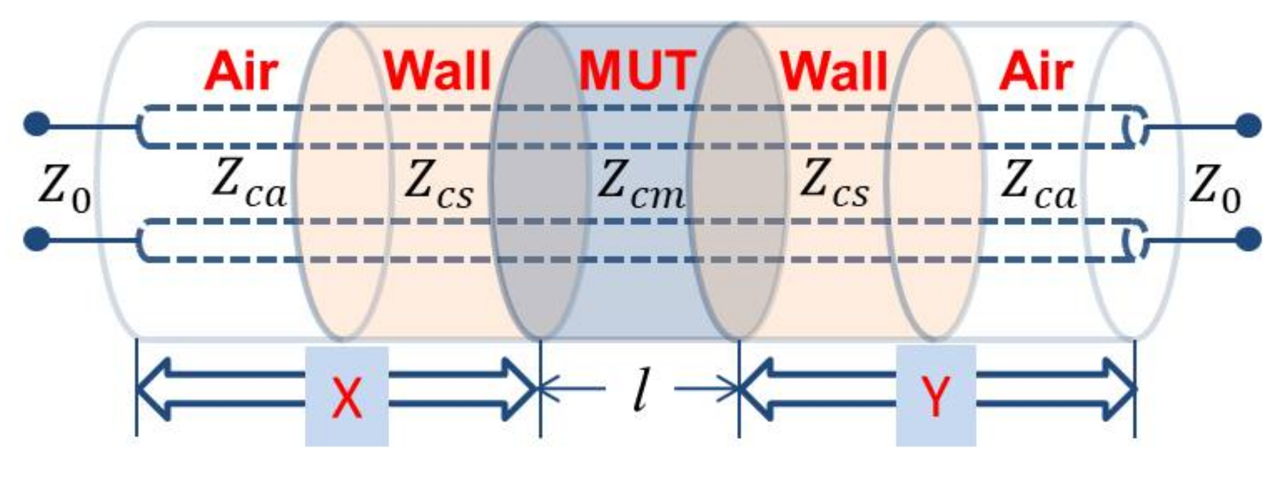
2.1. Circuit Theory of the Sensing Device

A transmission line can be described with the following equation

$$S^{Z_c,Z_c}\left(l\right)=\left[\begin{array}{cc}0& e^{-\gamma ·l}\\ e^{-\gamma ·l}& 0\end{array}\right]$$

(1)

where $Z_c$ is its characteristic impedance, $\gamma$ represents the propagation constant, and l is the physical length of the transmission line. (1) is valid when the reference impedance $Z_0$ is equivalent to the transmission line’s characteristic impedance $Z_c$. As shown in Figure 1, the whole measurement device, where the MUT is loaded, consists of five cascading transmission-line sections, i.e., two bare-line parts, two mirofluidic channel wall parts, and the MUT part. For the measurement device herein discussed, the bare lines are covered by air and the microfluidic channel is made from SU-8. In order to demonstrate the relationships between the five sections, researchers usually use the cascade matrix T in the following way

$$M_{mut}=Q^{Z_0,Z_{ca}}{T}_{airL}{Q}^{Z_{ca},Z_{cs}}{T}_{su8L}{Q}^{Z_{cs},Z_{cm}}{T}_{mut}{Q}^{Z_{cm},Z_{cs}}{T}_{su8R}{Q}^{Z_{cs},Z_{ca}}{T}_{airR}{Q}^{Z_{ca},Z_0}$$

(2)

where $Z_0$ is the reference impedance of the vector-network-analyzer (VNA) measurement system; $Z_{ca}$, $Z_{cs}$, and $Z_{cm}$ are the characteristic impedance of the air-covered transmission lines, SU-8 covered lines, and the MUT loaded line, respectively; $Q^{Z_0,Z_{ca}}$, $Q^{Z_{ca},Z_{cs}}$, $Q^{Z_{cs},Z_{cm}}$, $Q^{Z_{cm},Z_{cs}}$, $Q^{Z_{cs},Z_{ca}}$, and $Q^{Z_{ca},Z_0}$ are impedance transformers [38], which are defined by

$$Q^{Z_n,Z_m}={\displaystyle \frac{1}{2Z_m}}\left|{\displaystyle \frac{Z_m}{Z_n}}\right|\sqrt{{\displaystyle \frac{R\left(Z_n\right)}{R\left(Z_m\right)}}}\left[\begin{array}{cc}{Z}_m+Z_n& Z_m-Z_n\\ Z_m-Z_n& Z_m+Z_n\end{array}\right].$$

(3)

$T_{airL}$, $T_{su8L}$, $T_{mut}$, $T_{su8R}$, and $T_{airR}$ are the cascade matrices of the corresponding sections, whose reference impedance is the characteristic impedance of the corresponding transmission line; and M is the measured cascade matrix at the reference plane of the VNA measurement setup. The cascade matrices can be readily obtained from the corresponding S-parameters of a desired transmission line as in (1) and the measured S-parameters. By calculating the matrices and impedance transformers in (2) step by step, $T_{mut}$ can be extracted, and consequently, the permittivity of the MUT can be accurately characterized.

However, as can be seen, the above described step-by-step method is very time consuming, as much effort needs to be spent on calculating the intermediate parameters $Q^{Z_0,Z_{ca}}$, $T_{airL}$, $Q^{Z_{ca},Z_{cs}}$, etc. In order to simplify the extraction procedure, the measurement device, except the sensing section where the MUT is loaded, can be assumed as a test fixture. Thus, two de-embedding matrices X and Y can be used to demonstrate the effects of the test fixture. Then, (2) can by described as

$$M_{mut}=X·Q^{Z_0,Z_{cm}}{T}_{mut}{Q}^{Z_{cm},Z_0}·Y$$

(4)

where $T_{mut}$ is expressed as

$$T_{mut}=\left[\begin{array}{cc}{e}^{-{\gamma }_m·l_m}& 0\\ 0& e^{{\gamma }_m·l_m}\end{array}\right]$$

(5)

where $l_m$ is the length of the MUT covered part. Working as a reference, an empty device that has a corresponding length of $l_a$ but has the same cross-section and feeding part as the MUT loaded line is assumed. Similar to (4), the measured cascade matrix of the empty device can be described as

$$M_{air}=X·Q^{Z_0,Z_{ca}}{T}_{air}{Q}^{Z_{ca},Z_0}·Y.$$

(6)

Hence, using the line–line method [35], (4) and (6) can be combined in the following way

$$\begin{array}{cc}\hfill M_{mut}·M_{air}^{-1}& =\left[X·Q^{Z_0,Z_{cm}}·T_{mut}·Q^{Z_{cm},Z_0}·Y\right]·{\left[X·Q^{Z_0,Z_{ca}}·T_{air}·Q^{Z_{ca},Z_0}·Y\right]}^{-1}\hfill \\ \hfill & =X·Q^{Z_0,Z_{cm}}·T_{mut}·Q^{Z_{cm},Z_0}·{\left[Q^{Z_{ca},Z_0}\right]}^{-1}·{\left[T_{air}\right]}^{-1}·{\left[Q^{Z_0,Z_{ca}}\right]}^{-1}·X^{-1}.\hfill \end{array}$$

(7)

It is readily validated from the impedance transformer expression of (3) that ${\left[Q^{Z_n,Z_m}\right]}^{-1}$ equals $\left[Q^{Z_m,Z_n}\right]$; thus, (7) can be simplified as

$$\begin{array}{cc}\hfill M_{mut}·M_{air}^{-1}& =X·Q^{Z_0,Z_{cm}}·T_{mut}·Q^{Z_{cm},Z_0}·Q^{Z_o,Z_{ca}}·{\left[T_{air}\right]}^{-1}·Q^{Z_{ca},Z_0}·X^{-1}\hfill \\ \hfill & =X·Q^{Z_0,Z_{cm}}·T_{mut}·Q^{Z_{cm},Z_{ca}}·{\left[T_{air}\right]}^{-1}·Q^{Z_{ca},Z_0}·X^{-1}.\hfill \end{array}$$

(8)

From the law of similar matrices having the same determinant and the same trace, we have the following trace relationship due to its convenience of calculation

$$Tr(M_{mut}·M_{air}^{-1})=Tr\left(\left\{Q^{Z_0,Z_{cm}}·T_{mut}·Q^{Z_{cm},Z_{ca}}·{\left[T_{air}\right]}^{-1}·Q^{Z_{ca},Z_0}\right\}\right)$$

(9)

where $Tr(•)$ denotes the trace operation. If the term in $\left\{\right\}$ in (9) is defined as $TT$, after some manipulations with (3) and (5), $TT$ becomes

$$TT=\frac{1}{4}\left[\begin{array}{cc}T{T}_{11}& T{T}_{12}\\ T{T}_{21}& T{T}_{22}\end{array}\right]$$

(10)

where

$$\begin{array}{cc}\hfill T{T}_{11}=& 4cosh\left({\gamma }_m{l}_m\right)cosh\left({\gamma }_a{l}_a\right)-2\left(\frac{Z_{ca}}{Z_{cm}}+\frac{Z_{cm}}{Z_{ca}}\right)sinh\left({\gamma }_m{l}_m\right)sinh\left({\gamma }_a{l}_a\right)\hfill \\ \hfill & +2\left(\frac{Z_{ca}}{Z_0}+\frac{Z_0}{Z_{ca}}\right)cosh\left({\gamma }_m{l}_m\right)sinh\left({\gamma }_a{l}_a\right)-2\left(\frac{Z_{cm}}{Z_0}+\frac{Z_0}{Z_{cm}}\right)sinh\left({\gamma }_m{l}_m\right)cosh\left({\gamma }_a{l}_a\right)\hfill \\ \hfill T{T}_{12}=& 2\left(\frac{Z_{ca}}{Z_{cm}}-\frac{Z_{cm}}{Z_{ca}}\right)sinh\left({\gamma }_m{l}_m\right)sinh\left({\gamma }_a{l}_a\right)\hfill \\ \hfill & -2\left(\frac{Z_{ca}}{Z_0}-\frac{Z_0}{Z_{ca}}\right)cosh\left({\gamma }_m{l}_m\right)sinh\left({\gamma }_a{l}_a\right)+2\left(\frac{Z_{cm}}{Z_0}-\frac{Z_0}{Z_{cm}}\right)sinh\left({\gamma }_m{l}_m\right)cosh\left({\gamma }_a{l}_a\right)\hfill \\ \hfill T{T}_{21}=& 2\left(\frac{Z_{ca}}{Z_{cm}}-\frac{Z_{cm}}{Z_{ca}}\right)sinh\left({\gamma }_m{l}_m\right)sinh\left({\gamma }_a{l}_a\right)\hfill \\ \hfill & +2\left(\frac{Z_{ca}}{Z_0}-\frac{Z_0}{Z_{ca}}\right)cosh\left({\gamma }_m{l}_m\right)sinh\left({\gamma }_a{l}_a\right)-2\left(\frac{Z_{cm}}{Z_0}-\frac{Z_0}{Z_{cm}}\right)sinh\left({\gamma }_m{l}_m\right)cosh\left({\gamma }_a{l}_a\right)\hfill \\ \hfill T{T}_{22}=& 4cosh\left({\gamma }_m{l}_m\right)cosh\left({\gamma }_a{l}_a\right)-2\left(\frac{Z_{ca}}{Z_{cm}}+\frac{Z_{cm}}{Z_{ca}}\right)sinh\left({\gamma }_m{l}_m\right)sinh\left({\gamma }_a{l}_a\right)\hfill \\ \hfill & -2\left(\frac{Z_{ca}}{Z_0}+\frac{Z_0}{Z_{ca}}\right)cosh\left({\gamma }_m{l}_m\right)sinh\left({\gamma }_a{l}_a\right)+2\left(\frac{Z_{cm}}{Z_0}+\frac{Z_0}{Z_{cm}}\right)sinh\left({\gamma }_m{l}_m\right)cosh\left({\gamma }_a{l}_a\right).\hfill \end{array}$$

(11)

Hence, (9) is transformed to

$$Tr(M_{mut}·M_{air}^{-1})=2cosh\left({\gamma }_m{l}_m\right)cosh\left({\gamma }_a{l}_a\right)-\left(\frac{Z_{ca}}{Z_{cm}}+\frac{Z_{cm}}{Z_{ca}}\right)sinh\left({\gamma }_m{l}_m\right)sinh\left({\gamma }_a{l}_a\right)$$

(12)

This is the foundation of the proposed simple and fast complex permittivity extraction algorithm. For the characterization method herein used, (12) can be further simplified to minimize the calculation of intermediate parameters.

2.2. Characterization Algorithm

Four per unit length (p.u.l) parameters, i.e., resistance R, inductance L, capacitance C, and shunt conductance G [38], are usually used to model a transmission line. These distributed parameters are uniformly distributed along the line and are determined by the structure and dimensions of its cross-section. The four p.u.l parameters of a transmission line have the following relationship with its $\gamma$ and $Z_c$

$$\begin{array}{cc}\hfill \gamma & =\sqrt{(R+j\omega L)(G+j\omega C)}\hfill \end{array}$$

(13a)

$$\begin{array}{cc}\hfill Z_c& =\sqrt{(R+j\omega L)/(G+j\omega C)}.\hfill \end{array}$$

(13b)

In addition, values of R and L are related to the properties of the conductor, while values of C and G are related to the properties of the dielectric materials around the conductor [39]. Therefore, for the sensing device herein discussed, R and L at the sensing area should be the same at every frequency of interest before and after loading the MUT [28,33].

Hence, according to (13), we can have

$${\gamma }_m{Z}_{cm}={\gamma }_a{Z}_{ca}.$$

(14)

Hence, the ratios of characteristic impedance in (12) can be replaced by the corresponding inverse ratios of propagation constant, leading to

$$Tr(M_{mut}·M_{air}^{-1})=2cosh\left({\gamma }_m{l}_m\right)cosh\left({\gamma }_a{l}_a\right)-\left(\frac{{\gamma }_m}{{\gamma }_a}+\frac{{\gamma }_a}{{\gamma }_m}\right)sinh\left({\gamma }_m{l}_m\right)sinh\left({\gamma }_a{l}_a\right)$$

(15)

from which ${\gamma }_m$ can be readily obtained if $l_m$, ${\gamma }_a$, and $l_a$ are known [35].

It has been demonstrated in the previous research that the p.u.l capacitance and conductance have the following linear relationship with the complex permittivity of the dielectric materials around the transmission line conductor [6]

$$\begin{array}{cc}\hfill C_m& ={\epsilon }_0\left[P_1+P_2(\mathrm{Re}\left({\epsilon }_{r,s}^{*}\right)-1)+P_3(\mathrm{Re}\left({\epsilon }_{r,m}^{*}\right)-1)\right]\hfill \end{array}$$

(16a)

$$\begin{array}{cc}\hfill G_m& =\omega {\epsilon }_0\left[P_2\mathrm{Im}\left({\epsilon }_{r,s}^{*}\right)+P_3\mathrm{Im}\left({\epsilon }_{r,m}^{*}\right)\right]\hfill \end{array}$$

(16b)

where ${\epsilon }_{r,s}^{*}$ and ${\epsilon }_{r,m}^{*}$ are the relative complex permittivity of the line substrate and the MUT loaded on top of the sensing area, respectively; ${\epsilon }_0=8.8542·{10}^{-12}$ F/m is the vacuum permittivity; $P_1$, $P_2$, and $P_3$ are three coefficients, which are only determined by the geometry of the CPW transmission line. In practical applications, $P_1$, $P_2$, and $P_3$ can be obtained by calculation using the conformal method [6], finite-element-simulation method [27], or reference material measurement method [11]. Therefore, when ${\epsilon }_{r,s}^{*}$ is known, ${\epsilon }_{r,m}^{*}$ can be accurately obtained from the p.u.l capacitance $C_m$ and conductance $G_m$. Since R and L stay constant at every frequency before and after loading MUT, according to the relationship of propagation constant $\gamma$ with C and G in (13), we have

$$G_m+j\omega C_m=(G_m+j\omega C_a)·\frac{{\gamma }_m^2}{{\gamma }_a^2}.$$

(17)

Thus, the MUT-related capacitance $C_m$ and conductance $G_m$ can be readily obtained if the bare line capacitance $C_a$ and conductance $G_a$ are known. Therefore, in the proposed algorithm, only $G_a$, $C_a$, ${\gamma }_a$ and dimensions at the sensing area are required to be known in advance. Except for these, no other intermediate parameters need to be calculated.

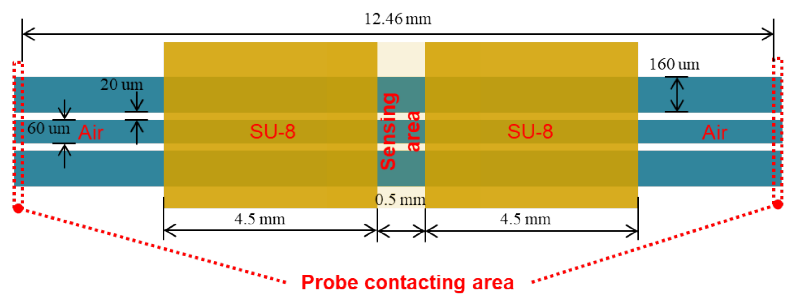
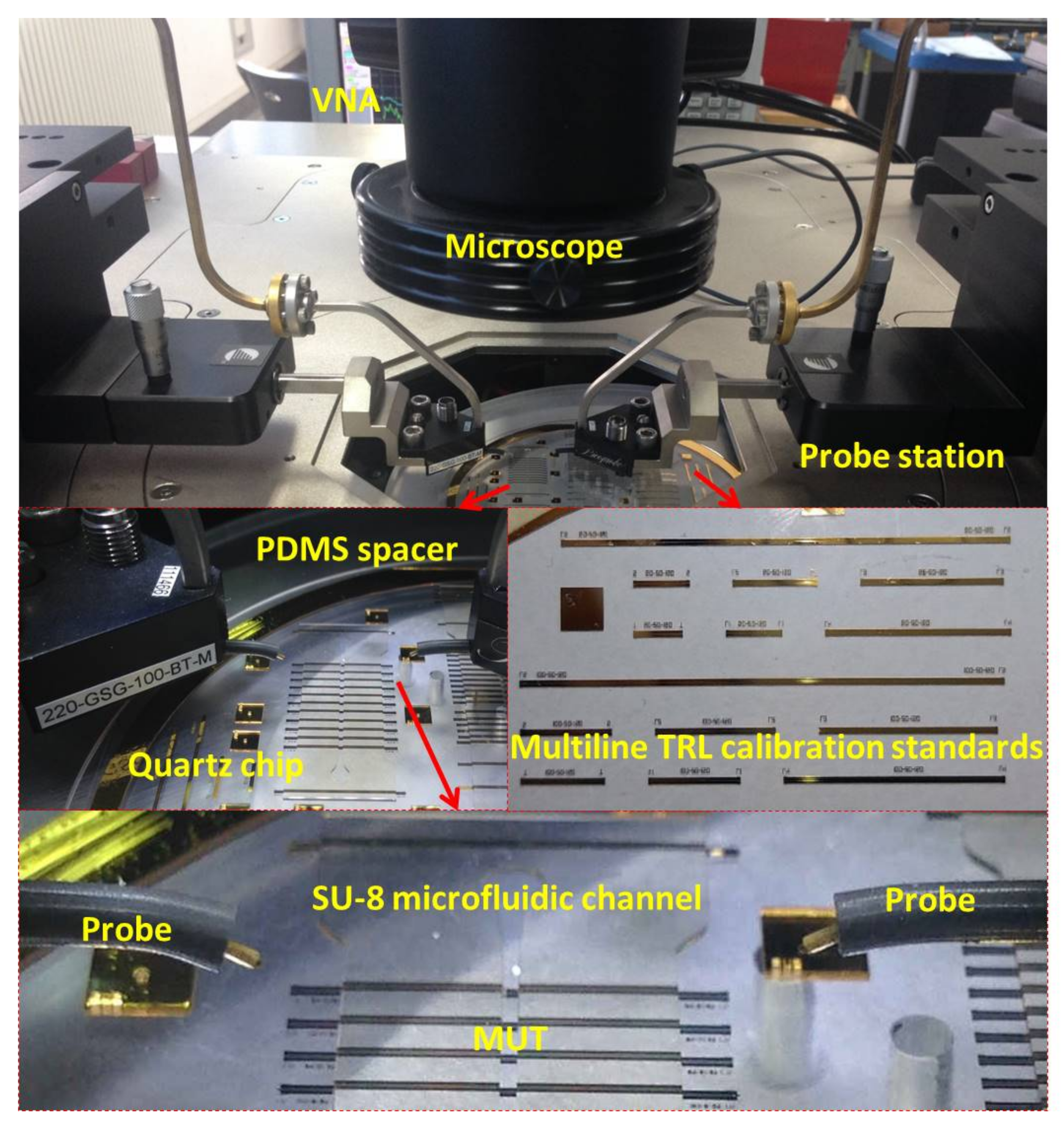
3. Device Fabrication and Measurements

The CPW sensing structure is fabricated on a 4-inch quartz (${\epsilon }_r$ = 3.78 and $tan\delta$ = 0.0001 at 10 GHz and 25 ${}^{°}\mathrm{C}$) wafer. On the surface of the quartz wafer, 650 nm thick Ti/Au CPW electrodes are deposited by the sputtering method and the lift-off technique. The fabrication procedure has been previously described in detail [40]. Dimensions of the CPW cross-section are 60 $\mathsf{\mu }$m conductor width (w), 20 $\mathsf{\mu }$m spacing width (s), and 160 $\mathsf{\mu }$m width of the ground plane (g), respectively, and the total length of the CPW line is $12.46$ mm. Next, a 400 $\mathsf{\mu }$m high and 500 $\mathsf{\mu }$m wide SU-8 microfluidic channel is patterned on top of the CPW electrodes. Thus, $l_m$ and $l_a$ are both 500 $\mathsf{\mu }$m in (15) for the validation measurements. The channel, where the MUT is flowing, is located perpendicular to the CPW electrodes. Widths of the channel walls are both $4.5$ mm. The structure and dimensions of the designed CPW TL device are shown in Figure 2.

Some calibration CPW lines that have different lengths and a calibration CPW short circuit are also lithographically patterned on the quartz wafer, using exactly the same fabrication procedure of the CPW sensing line. The cross-section of these CPW structures is 60 $\mathsf{\mu }$m–20 $\mathsf{\mu }$m–160 $\mathsf{\mu }$m (w-s-g) as well. The length of the CPW feeding part on either side of the short circuit is $1.75$ mm. For the frequency band of 140–220 GHz, the center frequency is 180 GHz, whose quarterwave line length is calculated by using $l=300/(4\times f_0\times \sqrt{({\epsilon }_r+1)/2})$, at $0.267$ mm. Therefore, two calibration CPW lines who have a length difference of $0.267$ mm work well in the frequency range between 40 and 320 GHz. The lengths of the calibration bare CPW lines are designed at $3.5$ mm, $3.767$ mm, 4 mm, 6 mm, 10 mm, and 13 mm, respectively. Thus, the length differences of any two calibration lines include $0.233$ mm, $0.267$ mm, $0.5$ mm, $1.3$ mm, 2 mm, $2.233$ mm, $2.5$ mm, 3 mm, 4 mm, 6 mm, $6.233$ mm, $6.5$ mm, 7 mm, 9 mm, $9.233$ mm, and $9.5$ mm. Hence, the calibration standards can perfectly cover the frequency band from about 5 GHz to approximately 370 GHz.

Figure 3 presents the on-wafer measurement setup and the fabricated quartz chip. An Agilent E8364B VNA and a pair of 220-GSG-100-BT-M picoprobes based on a manual probe station are used for the on-wafer measurements. For both the Mutliline-TRL calibration and the practical measurements of the bare sensing CPW line and the DI water loaded CPW line, 201 frequency points are collected in a linear approach. In order to reduce the excitation of the parasitic microstrip mode between the CPW conductors and the metal chuck, an 8 mm-thick plexiglass (${\epsilon }_r$ = 2.593 and $tan\delta$ = 0.022 around 10 GHz) spacer is placed under the quartz wafer when on-wafer measurements are performed. Before any practical measurements, a multiline thru-reflect-line (multiline-TRL) calibration process [41] is performed using the designed bare CPW lines and the CPW short circuit. With the help of a multiline-TRL calibration package [42], errors caused by cables and adapters between VNA and the probe tips can be precisely determined. Next, two groups of S-parameters are measured on the CPW sensing line, including the empty device (i.e., with air in the microfluidic channel) and the device after loading de-ionized (DI) water [43]. DI water can be readily injected into the SU-8 microfluidic channel by using a pipette. During the on-wafer measurements, the temperature of DI water is kept at approximately 25 ${}^{°}$C.

With the help of multiline-TRL calibration, the actual S-parameters of the complete CPW sensing line, before and after loading the MUT, can be accurately obtained. Additionally, based on the multiline-TRL calibration algorithm, the propagation constant of the calibration CPW lines, which is equivalent to the propagation constant ${\gamma }_a$ of the empty sensing CPW line, can be precisely obtained. Therefore, the propagation constant ${\gamma }_m$ of the DI water loaded CPW line is readily extracted by using (15). Next, by using the finite element method (FEM) on a bare CPW line that has exactly the same geometry and material property, the p.u.l capacitance $C_a$ of the bare line is obtained as 0.7693 pF/cm. The p.u.l conductance $G_a$ is assumed to be zero, since the loss of quartz substrate is negligible. Then, according to the theoretical analysis in the last section, $C_m$ and $G_m$ can be accurately extracted. By using the finite element simulation method, the three coefficients $P_1$, $P_2$, and $P_3$ in (16) are accurately obtained, and finally, ${\epsilon }_m^{*}$ can be accurately extracted based on

$${\epsilon }_m^{*}=\left(\frac{C_m-C_a}{1.669\times {10}^{-11}}+1\right)-j\frac{G_m}{1.669\times {10}^{-11}\omega }.$$

(18)

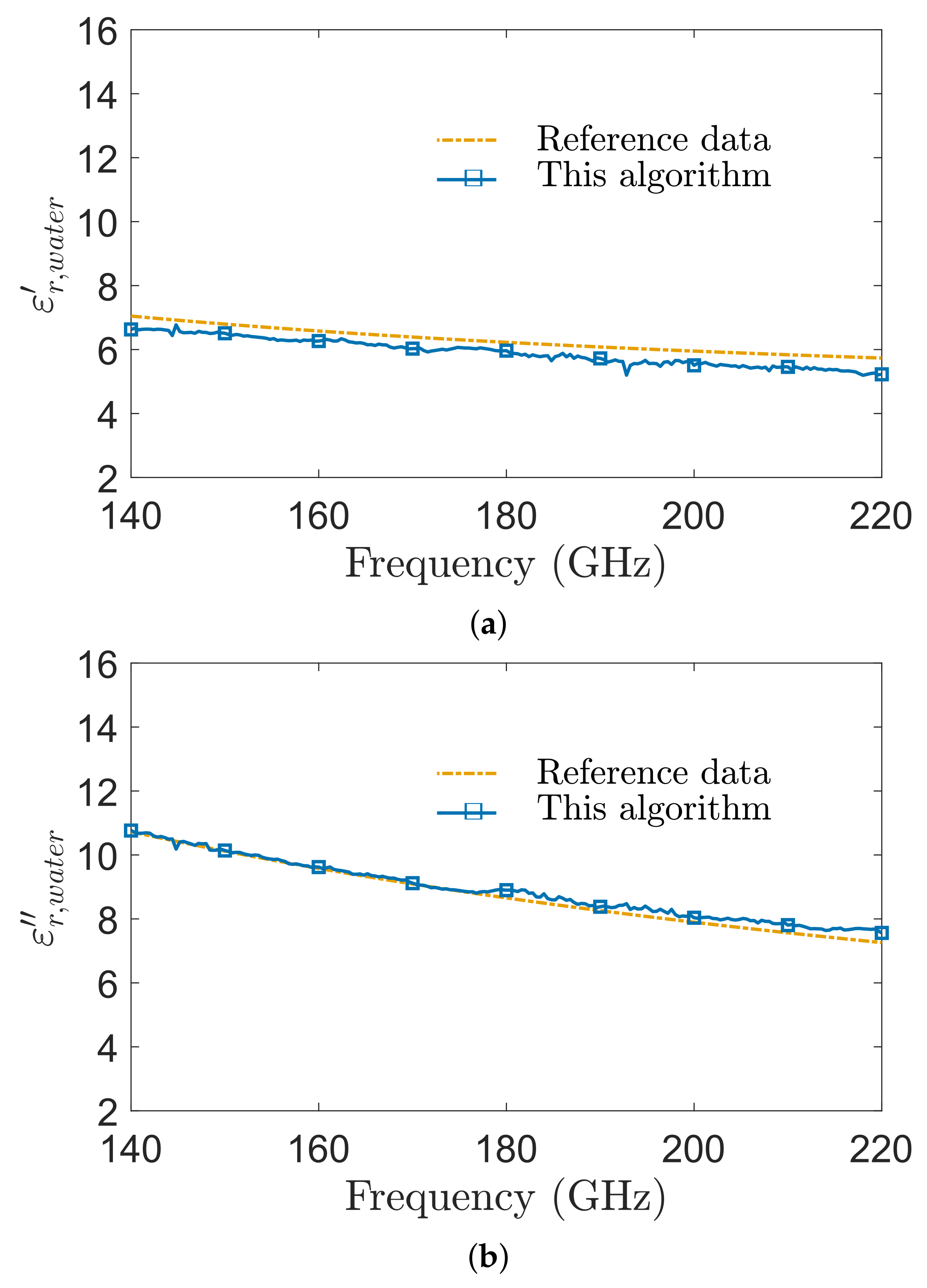
4. Results and Discussion

The measured permittivity results of DI water are presented in Figure 4. The corresponding data of water, which are calculated according to the following Double-Debye function [43], are also added in Figure 4.

$${\epsilon }_r^{*}={\epsilon }_{\infty }+{\Delta }_1/(1-j\omega {\tau }_1)+{\Delta }_2/(1-j\omega {\tau }_2)$$

(19)

where

$$\begin{array}{cc}\hfill {\epsilon }_{\infty }& ={\epsilon }_s-{\Delta }_1-{\Delta }_2,\hfill \\ \hfill {\epsilon }_s& =87.9144-0.404399·T+9.58726\times {10}^{-4}·T^2-1.32892\times {10}^{-6}·T^3,\hfill \\ \hfill {\Delta }_1& =a_1·exp(-b_1·T),\hfill \\ \hfill {\Delta }_2& =a_2·exp(-b_2·T),\hfill \\ \hfill {\tau }_1& =c_1·exp(d_1/(T+t_c)),\hfill \\ \hfill {\tau }_2& =c_2·exp(d_2/(T+t_c)).\hfill \end{array}$$

(20)

in which T is the actual temperature of DI water in ${}^{°}$C during the measurement procedure. The other coefficients used in (20) are listed in

Table 1. Coefficient values of the Double-Debye function for calculating the frequency- and temperature-dependent complex permittivity of water.

Coefficient	Value	Coefficient	Value	Coefficient	Value
$a_1$	79.42385	$a_2$	3.611638	$t_c$	132.6248
$b_1$	0.004319728	$b_2$	0.01231281
$c_1$	1.352835 × ${10}^{-13}$	$c_2$	1.005472 × ${10}^{-14}$
$d_1$	653.3092	$d_2$	743.0733

. It is clearly shown in Figure 4 that there is a very good agreement between the measurement results and the reference data. This has validated that the proposed simple algorithm can provide accurate and reliable measurement results of liquids’ complex permittivity. It should be noted that although the proposed method is validated within the frequency range from 140 to 220 GHz, it can be applied to both lower and higher frequencies [44], as long as either the electrical length of the transmission lines or the dielectric properties of the surrounding materials are obviously different at the frequencies of interest. Since the effects of the feeding parts are not required to be investigated and most of the intermediate parameters are not computed in the code, only a few seconds are needed to obtain the complex permittivity of MUT once the raw measured S parameters are imported. Thus, the proposed algorithm is very fast in broadband permittivity extraction applications.

During the procedure of data processing, ${\gamma }_a$ is obtained from the multiline-TRL calibration process as described in the last section, $C_a$ is extracted using the finite element simulation method, and $G_a$ is zero. Therefore, according to (13), the p.u.l resistance R and inductance L can be extracted, whose frequency dependence is plotted in Figure 5. Although R and L are not necessarily calculated in the proposed fast and simple algorithm, it is interesting to discuss their performance at millimeter waves. As clearly shown in Figure 5, both R and L are slowly increasing with the frequency ranging from 140 to 220 GHz. This is slightly different from their behaviors at low frequencies, where R increases with increasing frequency, whereas L decreases with increasing frequency. Theoretically, their behaviors are related to the geometry, fabrication procedure, and materials’ property of the CPW TLs. Skin depth ${\delta }_s$ is calculated with

$${\delta }_s=\sqrt{\frac{2}{\omega {\mu }_0{\mu }_r\sigma }}$$

(21)

where the conductivity $\sigma$ (gold for the CPW lines herein used), the free-space permeability ${\mu }_0$, and the relative permeability of the CPW conductor are $4.1\times {10}^7$ S/m, $4\pi \times {10}^{-7}$ H/m, and 1, respectively. Hence, at 220 GHz, the skin depth of the conductor is approximately $167.6$ nm, which is about one-quarter the thickness of the fabricated CPW conductor, while the designed conductor thickness is equivalent to its skin depth at around 14.64 GHz. Therefore, it is reasonable that R is increasing within the frequency range of interest herein. L is also affected by the conductor skin depth when the conductor’s thickness is smaller than one-fifth of its skin depth. Moreover, during the analysis, the substrate’s permittivity ${\epsilon }_s^{*}$ is assumed to be constant; thus, the corresponding CPW TL $C_a$ and $G_a$ are constant and zero, respectively. This assumption is correct at low frequencies, but it might be slightly different at millimeter and terahertz frequencies. This means that the errors caused by the assumption on the substrate can be transferred to the extraction of L and R. Further detailed analysis is needed on the four p.u.l parameters of CPW TLs at high frequencies.

5. Conclusions

A simple, fast, and accurate complex permittivity characterization algorithm is proposed for broadband millimeter wave frequencies. In the developed algorithm, parameters related to the feeding air covered and microfluidic channel wall covered lines are not required to be extracted. In addition, impedance mismatches between different sections are carefully considered by using the impedance transformers and exact values of all intermediate parameters are no longer needed to be obtained, including the characteristic impedance at the CPW TL sensing section before and after loading MUT, the p.u.l resistance and the p.u.l inductance before and after loading MUT, and the actual scattering parameters at the sensing area before and after loading MUT.

Next, a quartz wafer-based CPW sensing line is fabricated. SU-8 polymer is used to integrate with the CPW line, forming a microfluidic channel for MUT flowing inside. An on-wafer measurement setup is built for the validation of the proposed broadband complex permittivity characterization algorithm. For accurate calibration and accurate characterization of the bare CPW line, several bare CPW lines are carefully designed and fabricated as well. On-wafer measurements were performed on de-ionized water within the broadband frequency range from 140 to 220 GHz. The extracted complex permittivity of water is in good agreement with the literature data, which successfully validates that the proposed simple and fast broadband characterization algorithm is accurate and reliable for millimeter waves. Although the reported experimental validation has been focused on de-ionized water as a case study, the proposed broadband characterization algorithm is of general validity and thus can be readily applied to other liquids as future work.

References

1. Yeo, J.; Lee, J.I. Slot-loaded microstrip patch sensor antenna for high-sensitivity permittivity characterization. Electronics 2019, 8, 502. [Google Scholar] [CrossRef] [Green Version]
2. Sethi, W.; Ibrahim, A.; Issa, K.; Albishi, A.; Alshebeili, S. A new approach to determining liquid concentration using multiband annular ring microwave sensor and polarity correlator. Electronics 2020, 9, 1616. [Google Scholar] [CrossRef]
3. Lee, J.S.; Lee, G.H.; Mohyuddin, W.; Choi, H.C.; Kim, K.W. Design of an ultra-wideband microstrip-to-slotline transition on low-permittivity substrate. Electronics 2020, 9, 1329. [Google Scholar] [CrossRef]
4. Kawarasaki, M.; Tanabe, K.; Terasaki, I.; Fujii, Y.; Taniguchi, H. Intrinsic enhancement of dielectric permittivity in (Nb + In) co-doped TiO2 single crystals. Sci. Rep. 2017, 7, 5351. [Google Scholar] [CrossRef] [Green Version]
5. Chang, T.; Zhang, X.; Zhang, X.; Cui, H.L. Accurate determination of dielectric permittivity of polymers from 75 GHz to 1.6 THz using both S-parameters and transmission spectroscopy. Appl. Opt. 2017, 56, 3287–3292. [Google Scholar] [CrossRef]
6. Bao, X.; Ocket, I.; Bao, J.; Liu, Z.; Puers, B.; Schreurs, D.M.P.; Nauwelaers, B. Modeling of coplanar interdigital capacitor for microwave microfluidic application. IEEE Trans. Microw. Theory Tech. 2019, 67, 2674–2683. [Google Scholar] [CrossRef]
7. Ivanov, A.; Agliullin, T.; Laneve, D.; Portosi, V.; Vorobev, A.; Nigmatullin, R.R.; Nasybullin, A.; Morozov, O.; Prudenzano, F.; D’Orazio, A.; et al. Design and characterization of a microwave planar sensor for dielectric assessment of vegetable oils. Electronics 2019, 8, 1030. [Google Scholar] [CrossRef] [Green Version]
8. Itami, G.; Sakai, O.; Harada, Y. Two-dimensional imaging of permittivity distribution by an activated meta-structure with a functional scanning defect. Electronics 2019, 8, 239. [Google Scholar] [CrossRef] [Green Version]
9. Chao, H.W.; Chen, H.H.; Chang, T.H. Measuring the complex permittivities of plastics in irregular shapes. Polymers 2021, 13, 2658. [Google Scholar] [CrossRef]
10. Ermilova, E.; Bier, F.F.; Hölzel, R. Dielectric measurements of aqueous DNA solutions up to 110 GHz. Phys. Chem. Chem. Phys. 2014, 16, 11256–11264. [Google Scholar] [CrossRef]
11. Bao, X.; Zhang, M.; Ocket, I.; Liu, Z.; Nauwelaers, B.; Schreurs, D. Impact of measurement uncertainty on modeling of dielectric relaxation in aqueous solutions. IEEE Trans. Microw. Theory Tech. 2021, 69, 4082–4092. [Google Scholar] [CrossRef]
12. Wang, H.C.; Zyuzin, A.; Mamishev, A.V. Measurement of coating thickness and loading using concentric fringing electric field sensors. IEEE Sens. J. 2013, 14, 68–78. [Google Scholar] [CrossRef]
13. Ma, J.; Wu, Z.; Xia, Q.; Wang, S.; Tang, J.; Wang, K.; Guo, L.; Jiang, H.; Zeng, B.; Gong, Y. Complex permittivity measurement of high-Loss biological material with improved cavity perturbation method in the range of 26.5–40 GHz. Electronics 2020, 9, 1200. [Google Scholar] [CrossRef]
14. Rocco, G.M.; Barmuta, P.; Bao, X.; Schreurs, D.; Bozzi, M. Efficient approach for dielectric permittivity measurements of liquids adopting a 3D-printed cavity resonator. Microw. Opt. Technol. Lett. 2021, 63, 2797–2802. [Google Scholar] [CrossRef]
15. Tiwari, N.; Jha, A.; Singh, S.; Akhter, Z.; Varshney, P.; Akhtar, M.J. Generalized multimode SIW cavity-based sensor for retrieval of complex permittivity of materials. IEEE Trans. Microw. Theory Tech. 2018, 66, 3063–3072. [Google Scholar] [CrossRef]
16. Bao, X.; Zhang, M.; Ocket, I.; Bao, J.; Kil, D.; Liu, Z.; Puers, R.; Schreurs, D.; Nauwelaers, B. Integration of interdigitated electrodes in split-ring resonator for detecting liquid mixtures. IEEE Trans. Microw. Theory Tech. 2020, 68, 2080–2089. [Google Scholar] [CrossRef]
17. Raveendran, A.; Raman, S. Complex permittivity extraction of planar dielectrics using a noninvasive microwave transmission line resonant technique. IEEE Trans. Instrum. Meas. 2021, 70, 1–8. [Google Scholar] [CrossRef]
18. Jiang, Q.; Yu, Y.; Zhao, Y.; Zhang, Y.; Liu, L.; Li, Z. Ultra-compact effective localized surface plasmonic sensor for permittivity measurement of aqueous ethanol solution with high sensitivity. IEEE Trans. Instrum. Meas. 2021, 70, 1–9. [Google Scholar] [CrossRef]
19. Crupi, G.; Bao, X.; Babarinde, O.J.; Schreurs, D.M.P.; Nauwelaers, B. Biosensor using a one-port interdigital capacitor: A resonance-based investigation of the permittivity sensitivity for microfluidic broadband bioelectronics applications. Electronics 2020, 9, 340. [Google Scholar] [CrossRef] [Green Version]
20. Shim, J.Y.; Chung, J.Y. Complex permittivity measurement of artificial tissue emulating material using open-ended coaxial probe. IEEE Sens. J. 2020, 20, 4688–4693. [Google Scholar] [CrossRef]
21. Casacuberta, P.; Muñoz-Enano, J.; Vélez, P.; Su, L.; Gil, M.; Martín, F. Highly sensitive reflective-mode defect detectors and dielectric constant sensors based on open-ended stepped-impedance transmission lines. Sensors 2020, 20, 6236. [Google Scholar] [CrossRef] [PubMed]
22. Gonçalves, F.J.F.; Pinto, A.G.; Mesquita, R.C.; Silva, E.J.; Brancaccio, A. Free-space materials characterization by reflection and transmission measurements using frequency-by-frequency and multi-frequency algorithms. Electronics 2018, 7, 260. [Google Scholar] [CrossRef] [Green Version]
23. Ghodgaonkar, D.; Varadan, V.; Varadan, V.K. Free-space measurement of complex permittivity and complex permeability of magnetic materials at microwave frequencies. IEEE Trans. Instrum. Meas. 1990, 39, 387–394. [Google Scholar] [CrossRef]
24. Janezic, M.D.; Williams, D.F. Permittivity characterization from transmission-line measurement. In Proceedings of the 1997 IEEE MTT-S International Microwave Symposium Digest, Denver, CO, USA, 8–13 June 1997; Volume 3, pp. 1343–1346. [Google Scholar]
25. Janezic, M.D.; Williams, D.F.; Blaschke, V.; Karamcheti, A.; Chang, C.S. Permittivity characterization of low-k thin films from transmission-line measurements. IEEE Trans. Microw. Theory Tech. 2003, 51, 132–136. [Google Scholar] [CrossRef]
26. Grenier, K.; Dubuc, D.; Poleni, P.E.; Kumemura, M.; Toshiyoshi, H.; Fujii, T.; Fujita, H. Integrated broadband microwave and microfluidic sensor dedicated to bioengineering. IEEE Trans. Microw. Theory Tech. 2009, 57, 3246–3253. [Google Scholar] [CrossRef]
27. Bao, X.; Ocket, I.; Bao, J.; Doijen, J.; Zheng, J.; Kil, D.; Liu, Z.; Puers, B.; Schreurs, D.; Nauwelaers, B. Broadband dielectric spectroscopy of cell cultures. IEEE Trans. Microw. Theory Tech. 2018, 66, 5750–5759. [Google Scholar] [CrossRef]
28. Booth, J.C.; Orloff, N.D.; Mateu, J.; Janezic, M.; Rinehart, M.; Beall, J.A. Quantitative permittivity measurements of nanoliter liquid volumes in microfluidic channels to 40 GHz. IEEE Trans. Instrum. Meas. 2010, 59, 3279–3288. [Google Scholar] [CrossRef]
29. Costa, F.; Borgese, M.; Degiorgi, M.; Monorchio, A. Electromagnetic characterisation of materials by using transmission/reflection (T/R) devices. Electronics 2017, 6, 95. [Google Scholar] [CrossRef] [Green Version]
30. Hasar, U.C.; Westgate, C.R. A broadband and stable method for unique complex permittivity determination of low-loss materials. IEEE Trans. Microw. Theory Tech. 2009, 57, 471–477. [Google Scholar] [CrossRef]
31. Minteer, S.D. Microfluidic Techniques: Reviews and Protocols; Springer Science & Business Media: Berlin/Heidelberg, Germany, 2006; Volume 321. [Google Scholar]
32. Stojanović, G.; Paroški, M.; Samardžić, N.; Radovanović, M.; Krstić, D. Microfluidics-based four fundamental electronic circuit elements resistor, inductor, capacitor and memristor. Electronics 2019, 8, 960. [Google Scholar] [CrossRef] [Green Version]
33. Liu, S.; Orloff, N.D.; Little, C.A.; Zhao, W.; Booth, J.C.; Williams, D.F.; Ocket, I.; Schreurs, D.M.P.; Nauwelaers, B. Hybrid characterization of nanolitre dielectric fluids in a single microfluidic channel up to 110 GHz. IEEE Trans. Microw. Theory Tech. 2017, 65, 5063–5073. [Google Scholar] [CrossRef]
34. Lee, M.Q.; Nam, S. An accurate broadband measurement of substrate dielectric constant. IEEE Microw. Guid. Wave Lett. 1996, 6, 168–170. [Google Scholar]
35. Bao, X.; Liu, S.; Ocket, I.; Bao, J.; Schreurs, D.; Zhang, S.; Cheng, C.; Feng, K.; Nauwelaers, B. A general line–line method for dielectric material characterization using conductors with the same cross-sectional geometry. IEEE Microw. Wirel. Components Lett. 2018, 28, 356–358. [Google Scholar] [CrossRef]
36. Farcich, N.J.; Salonen, J.; Asbeck, P.M. Single-length method used to determine the dielectric constant of polydimethylsiloxane. IEEE Trans. Microw. Theory Tech. 2008, 56, 2963–2971. [Google Scholar] [CrossRef]
37. Lorenz, H.; Despont, M.; Fahrni, N.; LaBianca, N.; Renaud, P.; Vettiger, P. SU-8: A low-cost negative resist for MEMS. J. Micromech. Microeng. 1997, 7, 121. [Google Scholar] [CrossRef]
38. Marks, R.B.; Williams, D.F. A general waveguide circuit theory. J. Res. Natl. Inst. Stand. Technol. 1992, 97, 533–562. [Google Scholar] [CrossRef]
39. Williams, D.F.; Marks, R.B. Accurate transmission line characterization. IEEE Microw. Guid. Wave Lett. 1993, 3, 247–249. [Google Scholar] [CrossRef]
40. Bao, X.; Bao, J.; Ocket, I.; Liu, S.; Schreurs, D.; Kil, D.; Liu, Z.; Zhang, M.; Puers, R.; Nauwelaers, B. A simplified dielectric material characterization algorithm for both liquids and solids. IEEE Trans. Electromagn. Compat. 2018, 61, 1639–1646. [Google Scholar] [CrossRef]
41. Marks, R.B. A multiline method of network analyzer calibration. IEEE Trans. Microw. Theory Tech. 1991, 39, 1205–1215. [Google Scholar] [CrossRef] [Green Version]
42. Williams, D. StatistiCAL Software Package; National Institute of Standards and Technology: Gaithersburg, MA, USA.
43. Ellison, W. Permittivity of pure water, at standard atmospheric pressure, over the frequency range 0–25 THz and the temperature range 0–100 °C. J. Phys. Chem. Ref. Data 2007, 36, 1–18. [Google Scholar] [CrossRef]
44. Bao, X.; Liu, S.; Ocket, I.; Bao, J.; Kil, D.; Zhang, M.; Puers, B.; Schreurs, D.; Nauwelaers, B. A multiline multimaterial calibration method for liquid characterization. IEEE Microw. Wirel. Compon. Lett. 2018, 28, 732–734. [Google Scholar] [CrossRef]
Figure 1. A transmission-line-based sensing device, with the material under test being contained in a microfluidic channel formed by SU-8 polymer walls.
Electronics 11 00366 g001
Figure 2. The structure and dimensions of the designed CPW TL sensing device.
Electronics 11 00366 g002
Figure 3. On-wafer measurement setup, including the probe station, the microfluidic sensing chip, and the multiline-TRL calibration standards.
Electronics 11 00366 g003
Figure 4. The extracted real part (a) and imaginary part (b) complex permittivity of de-ionized water within the broadband millimeter wave frequency range between 140 and 220 GHz, using the proposed fast and simple characterization algorithm.
Electronics 11 00366 g004
Figure 5. Frequency dependence of the extracted per-unit-length resistance R (a) and the extracted per-unit-length inductance L (b) within the frequency range from 140 to 220 GHz.
Electronics 11 00366 g005aElectronics 11 00366 g005b