Abstract
Centralized control of voltage magnitude and reactive power (Volt-VAr) is a highly complex combinatorial problem that seeks to determine the optimal adjustment of a set of control variables such as active and reactive power generation of distributed generators (DGs), modules in operation of capacitor banks, and voltage regulator taps; these with the purpose of ensuring an optimal operation of distribution systems. Looking for tools that allow real-time automation of this type of control, this study applies different intelligent system (ISs) techniques, such as decision trees, artificial neural networks, and support vector machines. Voltage magnitudes at nodes, current flow magnitudes in the circuits, and active and reactive power injections at the nodes at different grid points were used as input data. Training was performed from available measurements and actions recorded at the system control center. The tests were performed in a 42-bus distribution test system demonstrating the efficiency and robustness of the proposed solution techniques when compared with the results of a conventional mathematical model.
1. Introduction
Within the smart grids context, one of the problems in electrical distribution systems (EDS) is the control of voltage magnitudes and reactive power (Volt-VAr), in which the objective is to determine the optimum adjustment of a set of control variables to ensure the proper operation of the EDS [1]. Among the main control variables, there are the active and reactive power generation of distributed generators (DGs), number of modules in operation of capacitor banks (CBs), and number of tap steps for on-load tap changer (OLTC) transformers as well as voltage regulators (VRs) [2]. Given its importance, and according to the smart grids philosophy, there is great interest in developing mechanisms that allow this control to be carried out automatically [3,4].
1.1. Literature Review
The Volt-VAr control has been extensively studied in the case where only OLTC transformers, VRs, and CBs modules are considered as control variables [5,6,7,8,9,10,11]. In [5], VRs taps are controlled cooperatively in real-time, after programming the optimal dispatch of CBs modules, using genetic algorithms (GAs). In [6], a dynamic programming algorithm is used to determine the optimal dispatch of VRs taps and CBs modules in order to minimize active power losses or voltage magnitude deviation of the system. In both [5,6], the impact of active and reactive DGs power injection on the Volt-VAr control is disregarded.
In [7], it is explained that the conventional control of the operation points of the CBs modules in radial grids need to be revised to include DGs in the feeders. In [8], the coordination of the taps of VRs and the modules of CBs is proposed to minimize active power losses in EDS considering DGs impact. In [9], a method of coordinated control of CB modules and taps of VRs is proposed. Although CBs, VRs, and DGs have a high presence in modern EDS, the optimal simultaneous adjustment of these control variables has not been fully studied. In fact, few works reported the coordinated control, considering all these elements, among which [10,11] stands out.
A common feature in several studies [5,6,7,8,9,10,11] is the need to know in detail the physical model of the EDS, that is, the need for a complete knowledge of the electrical parameters and the profile of the EDS demand. Nonetheless, such information is usually outdated, does not exist, cannot be easily estimated, or is not reliable [12].
In the trend of smart grids, modern EDS are migrating from an unsupervised and passive structure to a supervised and active one due to the installation of metering devices and the proliferation of digital protection systems [13,14]. In this context, the development of new control, monitoring, automation, and protection techniques is indispensable to meet the requirements of modern EDS. An important feature that these new techniques must incorporate concerns how to use relevant information from monitoring and metering systems available in several points of the electrical grid, which can be collected and stored for use in centralized and optimized decision making. An important benefit that may be obtained from this structure is the optimal centralized control of voltage magnitude and reactive power [15,16,17,18].
Therefore, intelligent systems (ISs) can be applied with the intention of managing a control system that allows a proper operation of EDS. ISs are built by extracting knowledge from a human expert and encoding it so that it can be applied to similar problems with a computer. ISs attempt to model human abilities through computational systems to find and interpret problem-response patterns. An IS characteristic is that its strategy for solving problems is dependent on the knowledge of an expert in the subject [19]. Among the methodologies belonging to ISs, there are artificial neural networks (ANNs), decision trees (DTs), and support vector machines (SVMs).
ANNs are able to computationally simulate human abilities such as learning, generalization, association, and abstraction. Thus, an ANN can be interpreted as a processing scheme capable of storing knowledge based on learning and making this knowledge available to its application. The use of ANNs to solve electrical energy systems problems is an area of growing interest [20]. In turn, DTs correspond to multistage decision-making approaches, which are widely used in many applications [21]. One of the main DTs characteristics is the ability to divide a complex decision process into a simpler set of decisions, providing successful solutions similar to the desired objectives [22]. SVMs are nonlinear models based on statistical learning theory. The main SVMs objective is to build an optimal decision function that, from a data set with expected inputs and outputs, classifies new inputs while minimizing the classification error [23].
1.2. Article Contribution and Organization
This work uses ANNs, DTs, and SVMs to determine the centralized control Volt-VAr in modern EDS by using electrical measurements. ISs define the most appropriate adjustment of the active and reactive power generation of DGs, the number of modules in operation of CBs, and the number of tap steps for OLTC and VRs, in order to minimize the active power losses of the system, using the measurements available in the control center. ISs can be trained from the available measurements and actions recorded at the system control center. However, a mixed-integer linear programming (MILP) model proposed in [10] is used to create this set of measurements and actions. The WEKA learning machine, version 3.7.10, is used to manage the three ISs. WEKA uses the multilayer perceptron/backpropagation learning algorithms, the J48/C4.5 and the SMO/PoliyKernel to perform the training of ANNs, DTs, and SVMs, respectively.
The main contributions of this work are as follows:
- *
- An alternative solution to the problem of centralized control Volt-VAR in modern ESD was proposed based on ISs techniques;
- *
- The proposed methodology allowed one to determine in a simplified way the solution of the centralized control problem Volt-VAR using different ISs techniques such as ANNs, DTs, and SVMs;
- *
- The software WEKA was used as an important computational tool to solve the problem of centralized Volt-VAR control.
The MILP model was implemented in AMPL mathematical modeling language [24] and was solved using the commercial CPLEX solver [25]. Several tests were performed using a benchmark distribution system to demonstrate the efficiency of the proposed solution techniques. The rest of the document is organized as follows: Section 2 presents a general overview of the Intelligent Systems implemented in the paper; Section 3 describes the proposed methodology for Volt-VAr centralized control; Section 4 presents the tests as results carried out on a 42-bus distribution test system; and finally, Section 5 presents the conclusions of the research.
2. Intelligent Systems
In the development of this work, we used a computational intelligence field known as ISs due to the strong expansion of electrical energy systems and the growing need for interdisciplinary cooperation. ISs have the ability to use knowledge to perform tasks or solve problems as well as harness associations and inferences to work with complex problems; furthermore, ISs have the ability to efficiently store and retrieve large amounts of information to solve problems or make decisions [26].
Within the ISs context, it is necessary to consider the meaning of “knowledge”; therefore, some assumptions and delimitation are necessary. In the first instance, one can think of levels of knowledge: facts, concepts, rules, and meta-rules. Knowledge may be represented as a combination of data structures and interpretive procedures that lead to a known behavior, which provides information to a system that can plan and decide [27].
The type of knowledge needed to solve existing problems determines which sources of information are used by individuals. Therefore, knowledge can be generated from the combination of different information. Thus, a decision can occur through logical analysis or be supported by heuristic or intuitive data [28].
The intelligent behavior of a system is the result of multiple chained decisions. The choice of decision or decision control is based on performance, duration, and risk criteria [29].
ISs can be developed using various techniques, which can be applied alone or together to help decision making. The main techniques and methodologies used by ISs are: knowledge acquisition, machine learning, ANNs, fuzzy logic, SVMs, evolutionary computing, agents, multiagents, and data and text mining. Each of these techniques offers a variety of degrees of ability to represent human knowledge. For the development of this research, three techniques were used: ANNs, DTs, and SVMs. These techniques were chosen due to the fact that they have proven to be successful in several areas, especially in electrical engineering applications as evidenced in [30,31,32,33].
2.1. Artificial Neural Networks
In ISs, ANNs are mathematical models that resemble biological neural structures and have computational capacity acquired through learning and generalization. Learning in ANNs consists of the phase in which the neural network uses pairs of input and output data to modify its learning parameters [20].
This step can be an ANN adaptation to the intrinsic characteristics of a problem, where covering a large spectrum of values associated to the relevant variables is intended. This is performed so that ANN acquires, through a gradual improvement, a proper capacity of response for the greater number of possible situations. In addition, the generalization of an ANN associates with its ability to provide coherent responses to data not presented to it during training. Therefore, a trained ANN is expected to have a good generalization capacity regardless of whether it has been controlled during training [34]. One of the main ANNs characteristics is the ability to acquire, store, and use experimental knowledge.
ANN structure is defined by the way in which these neurons are organized and interconnected: that is, the number of layers, number of neurons per layer, and types of connection between neurons and network topology, as shown in Figure 1 (adapted from [35]).
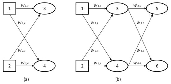
Figure 1.
(a) Simple neural network with two input nodes and two output nodes. (b) Simple neural network with two input nodes, one hidden layer with two nodes and two output nodes.
There are several models for implementing an ANN structure, such as SOM (self-organizing map), RBF (radius basis function), LMS (least mean square) and MLP (multilayer perceptron).
MLP is the ANN structure that we used in this study. These multilayer networks are distinguished from single-layer networks by the number of intermediate layers. This architecture has one or more hidden layers. According to [20], the hidden neuron function is to intervene between the external input layer and the network output in a useful way. By adding one or more hidden layers, the network is capable of extracting high-order statistics. This ability of hidden neurons is particularly valuable when the size of the input layer is large. Each layer of the MLP model has a specific function [34]:
- *
- Input layer: This is a noncomputational layer in which there is no processing; it is responsible for receiving and propagating input information to the next layer;
- *
- Hidden or intermediate layers: These are computational layers that perform processing; the information is transmitted to them through the connections between the input and output units. These connections save the weights that are multiplied by the inputs, ensuring the network knowledge;
- *
- Output layer: This is made of computational neurons and receives information from the hidden layers providing the response.
2.2. Decision Trees
A decision tree (DT) is a data structure defined recursively as a leaf node corresponding to a class and decision nodes that contain a test on some attribute. For each test, results correspond to an edge for a subtree. Each subtree has the same structure as the tree. DTs are used as a predictive model [36] that can classify and represent regression models. DTs are categorized as a supervised training method to find a logical connection between input attributes and the purpose of the attributes that represent the logical connection in structures as a model [37].
Figure 2, adapted from [38], depicts an example of a general DT for classification. The circles denote the root and internal nodes while the square denote the leaf nodes. In this particular example, the DT is designed for classification, and thus, the leaf nodes hold class labels.
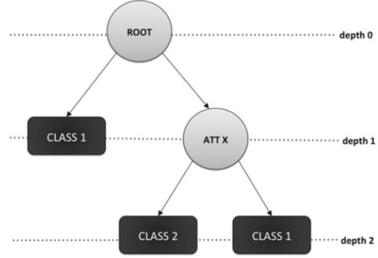
Figure 2.
General structure of a DT.
DTs are some of the most widely used and very popular techniques among searches due their simplicity, intelligibility, and ease of development. DTs construction is faster and more accurate than other classification algorithms. It is easy to observe that the tree can be represented as a set of rules. Each rule has its beginning at the root of the tree and moves toward one of its leaves. The key to success of the DTs learning algorithm depends on the criteria used to choose the attribute that divides the set of examples into each of the iterations [22].
DTs approach can be trained through several algorithms, which include J48, REPTree, PART, Ridor, and JRip, among others. In this research, we used the J48 algorithm that achieves a slightly higher correctness probability than the other classifiers. Algorithm J48 is a version of the traditional C4.5 algorithm, developed by J. Ross Quinlan [39]. This algorithm can process attributes of any type of input, through the discretization of numeric values by heuristics. However, the tree is not able to perform regression and plays only the role of the classifier; that is, the class attribute must be discrete [40].
2.3. Support Vector Machines
SVM theory is based on the idea of structural risk minimization, which has presented an excellent performance. According to [23], SVM structure is currently the most popular prefabricated approach for supervised learning, due to the following three properties: (a) SVMs construct a maximal margin separator; that is, a decision boundary with the longest possible distance to example points. Thus, allowing a correct generalization; (b) SVMs create a linear separation in hyperplane but have the capacity to incorporate the data in a space of superior dimension, using the so-called Kernel; and (c) SVMs are nonparametric methods; that is, they hold training examples and may need to store all of them. Thus, SVM combines the advantages of nonparametric and parametric models since they have the flexibility to represent complex functions but are resistant to overadaptation.
SVM is part of the family of linear classifiers, because they map the input points in a space of characteristics of a larger dimension to find the hyperplane that separates them and maximize the margin between classes. To separate two classes, the maximum margin separator is used; the margin is the width of the delimited area, and the separator is defined as a set of points . Thus, a separate hyperplane should not only classify the data correctly but should also make the margins as large as possible [41]. The SVM mathematical formulation varies depending on the nature of the data; therefore, there is a formulation for linear cases and another formulation for nonlinear cases.
Figure 3, adapted from [35], illustrates an SVM. On the left side, two classes of points can be seen (black and white circles), along with three candidate linear separators. On the right side, there is a separator which is at the midpoint of the margin, that is, the area between the dashed lines. The support vector, represented in Figure 3 as points with large circles, is the closest example of the separator [35].
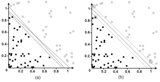
Figure 3.
(a) Two classes of points. (b) maximum margin separator.
However, real-world problems are generally not linearly separable, and this is where the Kernel method is introduced [42]. The Kernel function can be applied to pairs of input data to evaluate scalar products in some corresponding feature space. Thus, it is possible to learn in the higher dimension space, but only Kernel functions are calculated instead of a complete list of characteristics for each data point. According to [41], the intelligent Kernel trick is connected to the chosen Kernel.
Although the high-dimensional feature space (d-degree polynomials in the input space has free parameters), the dimension estimate of the subset of polynomials that solve practical problems (based on a given training set) can be low. If the expectation of this estimate is low, then the expectation of error probability is small [23].
SVMs have been developed as a robust technique for classification and regression applied to large complex and noise-rich data sets; that is, with variables inherent to the model that for other techniques increase the error possibility in the results, because they are difficult to quantify and observe. Further details on SVMs and the Kernel method can be found in [43].
3. Proposed Methodology
In this study, an ISs-based methodology is presented, which allows one to define the real-time centralized control of voltage magnitude and reactive power of an electrical distribution system, using electrical measurements as an input database. These data are submitted to a filtering process to later enter the intelligent system. The classification process is carried out within the ISs. Finally, the most appropriate adjustments of modules in operation of CBs, the number of tap steps of each OLTC transformer, and the active and reactive power injections from each DG unit are obtained. Figure 4 shows a diagram with the respective input and output variables of the IS.
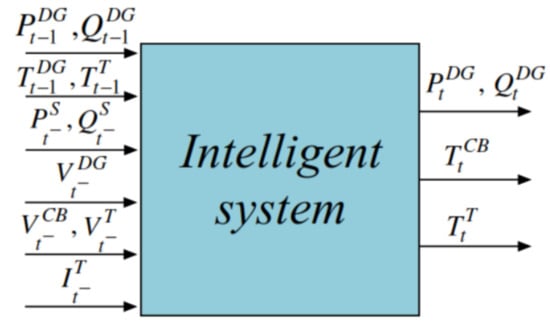
Figure 4.
Input and output variables of the proposed ISs.
In this case, and are vectors of active and reactive power injections of the distributed generation at time interval , is the vector of modules in operation of capacitor banks at time , is the vector of tap steps of transformers with on-load tap changers at time , and are the injection of active and reactive power of substation at time , is the vector of voltage magnitudes at nodes of distributed generators in operation at time t, is the vector of voltage magnitudes at the nodes of capacitor banks in operation at time t, and and are the vectors of voltage and current magnitudes at nodes controlled by transformers with on-load tap changers and voltage regulator in operation at time . On the other hand, the control actions in the time period t are: and , which correspond to the vectors of active and reactive power injections of distributed generation, , which indicates the vector of modules in operation of capacitor banks and , which indicates the tap steps of transformers with on-load tap changers.
Figure 5 shows a graphical representation of the steps required to create the database used to perform ISs training. At time period , the system is operating on a steady state with active and reactive demands given by and , respectively, and with values of control variables given by , , , and . Note that between time and t, there is a time labeled as ; this time is before the system control changes; that is, the controls defined in the time period remain fixed on while the demand varies. Given the controls defined in the fixed time period and the variation of demand (, ), a new operating point is defined in the system in time . This operating point can be calculated using a backward/forward sweep load flow [44].
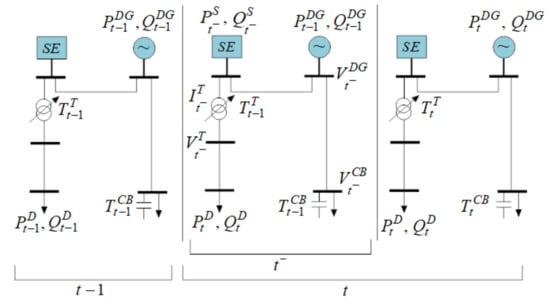
Figure 5.
Graphical representation of the steps used to create the database.
With the load flow (LF) result, it is possible to store all the information in the meters available in the system that can be accessed in the time interval . In this case, this information includes: , , , , , and . Thus, it is possible to obtain all the ISs input data. In the transition period between time and t, the demand of the system ( and ) remains constant. Control variables , , , and at time t are calculated using an MPLIM model presented in [10], which represents the ISs output data. In addition, the database of this work was created following the method proposed in [45].
In order to perform the IS training, it is necessary to create databases with all measurements of the system in time and control actions in time t. In this study, we carried out a system analysis for 365 days, hour by hour; therefore, a total of 8760 records was obtained. To apply this methodology, the WEKA machine learning platform was used.
Machine Learning Platform
Algorithm J48, MLP, and PoliKernel were implemented using the free software WEKA. This software has a wide variety of machine learning algorithms, developed in Java programming language, which are useful for being applied in databases making use of the interfaces it offers. In addition, WEKA contains the tools necessary to perform transformations on data, classification tasks, regressions, clustering, association, and visualization. WEKA is designed as an extensibility-oriented tool, meaning that adding new features is a simple task; furthermore, it is a freely distributed and multiplatform software that is made up of a series of open-source packages with different techniques; these packages can be integrated into any project of data analysis and can even be extended with contributions from users who develop new algorithms.
4. Tests and Results
The development of this work was performed considering a distribution network composed of 42 buses, with 5 CBs, 2 DGs, and 4 VRs. The single-line diagram shown in Figure 6 represents the configuration of the described system used in [10].
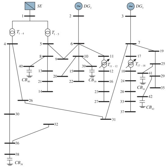
Figure 6.
42-bus distribution system diagram.
The data created from the MPLIM solution of the distribution system operation planning problem (POSD) and presented in [10] were used in this paper. The proposed model was implemented to determine active and reactive power injections of DGs, the number of capacitor modules in operation, and the number of tap steps of VRs, in order to minimize the cost of the system daily energy losses, as represented in the POSD objective function.
Through this mathematical model solution, a database was created with information of the system control data of 365 days, hour per hour (8760 records). This database considers a random variation of demand relative to a daily demand curve divided into one-hour intervals and is used to perform the training of DTs, SVMs, and ANNs.
In addition, four other databases were generated (also from the MILP model presented in [10]), which are made up of data with a history of system control records for 7 days, on an hourly basis (168 records). These data were used to carry out the validation of the three ISs; the difference between these four databases is the percentage of random variation in demand at , , , and . The data were analyzed with the software WEKA which allows one to perform the training and validation process of DTs, ANNs, and SVMs. According to the tests carried out with ISs, the training data presented a high level of veracity in their validation, which is analyzed in this section.
With each database used to perform the training and validation of DTs, SVMs, and ANNs, tests were performed in which the different parameters of each ISs were calibrated; one of the most critical cases were with ANNs, in which, after several tests in the training process, it can be seen how difficult it is to find the optimal adjustment of the training parameters that are needed when trying to achieve better results. These parameters are selected by using time and training error criteria and shown in Table 1. The calibration of ISs parameters is of utmost importance because they are directly related to the quality of the results obtained.

Table 1.
Parameters used for ANN training.
To perform the training of DTs, SVMs, and ANNs, a number of discretizations was considered; for DGs, a control measure of 20 was necessary, for CBs modules, a 4-control measure was performed, and for VRs taps a control measure of 2 and 16 units were necessary.
Table 2 shows the percentages of correct classification according to the crossvalidation test option chosen within the software WEKA to perform the ISs training and validation using data with random variation of demand ( and ).
Table 2.
Classification percentage using crossvalidation.
4.1. Case A—Validation Process Using Input Data Generated by the MILP Model
Considering that the random variation of demand of represents a greater computational effort, the performance of each proposed IS is compared for this particular case. In order to analyze this case, four databases were created with the history of energy losses of the system hour by hour during a week, to evaluate each one of the used ISs. Table 3 compares the results obtained by the ISs, and the results obtained after the simulation with the MPLIM model.
Table 3.
Comparison of daily energy losses results in KWh.
Thus, to validate the results, day 1 was chosen from this database, which is the day with the highest levels of energy losses. Table 4 shows a comparison of the hourly values of energy losses of the studied system, obtained by MPLIM and the three ISs for day 1, which is the day with the highest levels of demand and highest levels of energy losses.
Table 4.
Comparison of hourly energy loss results in kWh.
Figure 7 shows the power losses in the system for each time interval (control action defined by ISs for 24 h) for the demand variation percentage of . The values of the losses obtained using the optimum control action are the results obtained in the simulation of the conic MPLIM model, while the others correspond to the control action defined by the ISs.
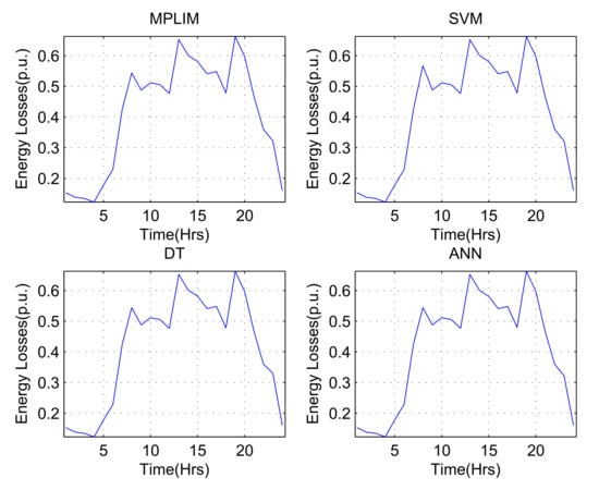
Figure 7.
Energy losses calculated for 24 h.
Figure 8 shows the minimum voltage in the system for each time interval (control action defined by the ISs for 24 h) for the demand variation percentage of .

Figure 8.
Minimum voltage calculated for 24 h.
4.2. Case B—Validation Process Using Load Flow Results as Input Data
In study case B, ISs are autonomous, and once they are trained, they receive the input database directly from the load flow and then return the control defined by the ISs; in this case, we considered the random variation of demand of to compare the performance of each IS proposed for this particular case. In order to analyze this case, four databases were created with the history of energy losses of the system hour by hour during a week, to evaluate each one of the ISs. Table 5 compares the results obtained by the ISs and the values calculated by the MPLIM model.
Table 5.
Comparison of daily energy losses results in KWh.
Day 2 was chosen to validate the results from this database, which is the day with the highest levels of energy losses. Table 6 shows a comparison of the hourly values of energy losses of the studied system, obtained by MPLIM and by the three ISs for the day that present higher levels of losses.
Table 6.
Comparison of hourly energy loss results in kWh.
Figure 9 shows the power losses in the system for each time interval (control action defined by ISs for 24 h) for a demand variation of . The values of the losses obtained using the optimum control action are the results obtained in the simulation of the conic MPLIM model, while the others correspond to the control action defined by the ISs.
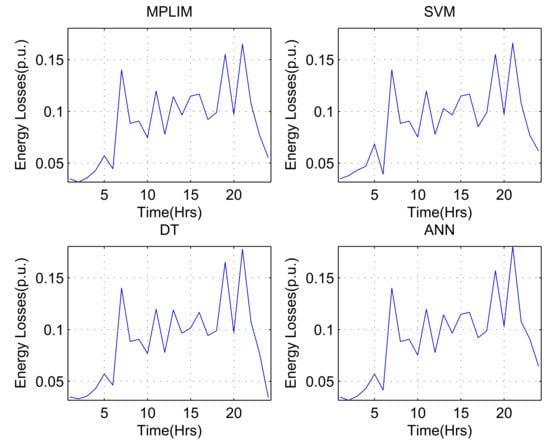
Figure 9.
Energy losses calculated for 24 h.
Figure 10 shows the minimum voltage in the system for each time interval (control action defined by the ISs for 24 h) for the demand variation percentage of .
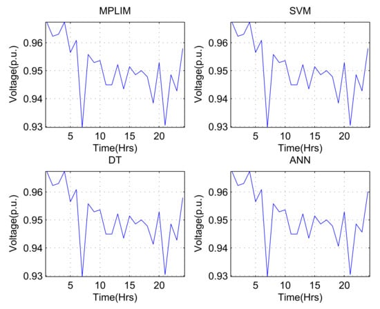
Figure 10.
Minimum voltage calculated for 24 h.
For a better analysis of this proximity, the values that allow quantifying prediction errors are presented in terms of absolute mean deviations (AMD). Table 7 shows the validation set with random variation, the AMD between discrete states, and the percentages of correctness for each of the control elements of the system (DGs, CBs, and VRs), when comparing the results assumed to be real (results obtained after the simulation of the MPLIM model) with the results obtained by the ISs.
Table 7.
Percentage of hits and AMD by variable for 20% variation in demand.
According to the results of Table 7, SVMs have better performance, with lower percentages of absolute mean deviations and higher percentages of correctness. In addition, the smallest correctness deviations for DTs, SVMs, and ANNs correspond to predictions of the injected powers by the DGs, however, with percentages that can be considered acceptable. Again, the results are acceptable, since, for the highest percentage of variation of demand , the percentages of correctness remains greater than with the three ISs.
Table 8, Table 9 and Table 10 present the number of predicted values using IS that presented better results, such as the SVM case; these values are classified according to the percentages of absolute mean deviations when compared with the real values, both for minimum voltages (in kV) and for system losses. Other information resulting from these simulations is the amount of predictions with infeasible results, which depend not on the IS but on the increase in demand variation. Therefore, 10, 21, and 33 results were obtained for percentages of demand variation of , , , and , respectively.
Table 8.
AMD of the values obtained (5% variation in demand).
Table 9.
AMD of the values obtained (10% variation in demand).
Table 10.
AMD of the values obtained (20% variation in demand).
Note that there is a significant amount of predicted results with absolute mean deviations between and indicated in Table 11, also in percentages. This shows the high proximity of the expected results when compared with the values assumed to be real.
Table 11.
Percentage of predicted results with AMD values between 0% and 20%.
5. Conclusions
In this work, the voltage magnitude and reactive power control problem was addressed using three ISs methodologies to determine the real-time centralized control of voltage and reactive power magnitude (Volt-VAr) of distribution systems using electrical measurements. The free software WEKA was used to train and evaluate the three ISs (DTs, SVMs, and ANNs) in the calculation of the operating points of DGs, CBs, and VRs.
The comparison between the results obtained in the solution of an MPLIM model with the objective of minimizing power losses, and the results obtained using ISs show low prediction errors that lead one to consider the use of these methodologies to be fast and efficient alternatives. The results show low errors compared to the those provided by a mathematical model, which evidences the usefulness of the proposed method.
According to the results presented by the IS-based methods, for the test conditions, the SVMs presented a better performance with lower AMD percentages and higher percentages of correctness. The lowest percentages of correctness, for DTs, SVMs, and ANNs (for random variation of demand), correspond to predictions of the injected powers by DGs but with percentages that can be considered acceptable.
For the three ISs, tests were performed for percentages of random variation of demand (, , , and ). The absolute mean deviations between discrete states and percentages of correctness are acceptable since, for example, for the highest percentage of variation of demand (), the percentages of correctness remains greater than .
The decision-making process can be carried out without the detailed representation of the network physical model, since measurement data can be used as input for IS training.
The ISs training times were reasonable considering the complexity of the Volt-VAr centralized control problem. In addition, the response times of a maximum of 1 second indicate that the time it takes for the ISs to obtain a solution to the problem is similar to that obtained by the devices used in real time.
Future research will include other ISs techniques such as machine learning, fuzzy logic, and evolutionary computing. Furthermore, the use of other benchmark distribution system will be considered along with the effect of distributed energy resources within the Volt-VAr control problem.
Author Contributions
Conceptualization, H.A.R.F., E.M.C.-F., and G.P.L.; data curation, H.A.R.F., E.M.C.-F., and G.P.L.; formal analysis, H.A.R.F., E.M.C.-F., G.P.L., N.M.-G., and J.M.L.-L.; funding acquisition, J.M.L.-L. and N.M.-G.; investigation, H.A.R.F., E.M.C.-F., and G.P.L.; methodology, H.A.R.F., E.M.C.-F., G.P.L., N.M.-G., and J.M.L.-L.; project administration, H.A.R.F., E.M.C.-F., G.P.L., N.M.-G., and J.M.L.-L.; resources, H.A.R.F., E.M.C.-F., G.P.L., N.M.-G., and J.M.L.-L.; software, H.A.R.F., E.M.C.-F., and G.P.L.; supervision, J.M.L.-L.; validation, H.A.R.F., E.M.C.-F., G.P.L., N.M.-G., and J.M.L.-L.; visualization, H.A.R.F., E.M.C.-F., G.P.L., N.M.-G., and J.M.L.-L.; writing—original draft, H.A.R.F., E.M.C.-F., and G.P.L.; writing—review and editing, H.A.R.F., E.M.C.-F., G.P.L., N.M.-G., and J.M.L.-L. All authors have read and agreed to the published version of the manuscript.
Funding
This research received no external funding.
Acknowledgments
The authors gratefully acknowledge the support from the Colombia Scientific Program within the framework of the call Ecosistema Científico (Contract No. FP44842- 218-2018). The authors also want to acknowledge the “estrategia de sostenibilidad” at Universidad de Antioquia in Medellín, Colombia, as well as the Department of Electrical Engineering (UTFPR) and the Academic Department of Computational Science (UTFPR) at Paraná, Brazil, for their support in the development of this work.
Conflicts of Interest
The authors declare no conflict of interest.
Nomenclature
The notation used throughout this paper is shown below for quick reference.
| Vector of active power injections of distributed generators in operation at time t. | |
| Vector of reactive power injections of distributed generators in operation at time t. | |
| Vector of modules in operation of capacitor banks at time t. | |
| Vector of tap steps of transformers with on-load tap changers at time t. | |
| Injection of active power of substation at time t. | |
| Injection of reactive power of substation at time t. | |
| Demand of active system power at time t. | |
| Demand of reactive system power at time t. | |
| Vector of voltage magnitudes at nodes of distributed generators in operation at time t. | |
| Vector of voltage magnitudes at nodes of capacitor banks in operation at time t. | |
| Vector of voltage magnitudes at nodes controlled by the transformers with tap changer under load and voltage regulator in operation at time t. | |
| Vector of current magnitudes in transformers with tap changer under load and voltage regulator in operation at time t. |
References
- Villa-Acevedo, W.M.; López-Lezama, J.M.; Valencia-Velásquez, J.A. A Novel Constraint Handling Approach for the Optimal Reactive Power Dispatch Problem. Energies 2018, 11, 2352. [Google Scholar] [CrossRef]
- Morán-Burgos, J.A.; Sierra-Aguilar, J.E.; Villa-Acevedo, W.M.; López-Lezama, J.M. A Multi-Period Optimal Reactive Power Dispatch Approach Considering Multiple Operative Goals. Appl. Sci. 2021, 11, 8535. [Google Scholar] [CrossRef]
- Bedawy, A.; Yorino, N.; Mahmoud, K.; Zoka, Y.; Sasaki, Y. Optimal Voltage Control Strategy for Voltage Regulators in Active Unbalanced Distribution Systems Using Multi-Agents. IEEE Trans. Power Syst. 2020, 35, 1023–1035. [Google Scholar] [CrossRef]
- Tushar, M.H.K.; Assi, C. Volt-VAR Control Through Joint Optimization of Capacitor Bank Switching, Renewable Energy, and Home Appliances. IEEE Trans. Smart Grid 2018, 9, 4077–4086. [Google Scholar] [CrossRef]
- Park, J.Y.; Nam, S.R.; Park, J.K. Control of a ULTC Considering the Dispatch Schedule of Capacitors in a Distribution System. IEEE Trans. Power Syst. 2007, 22, 755–761. [Google Scholar] [CrossRef]
- Liang, R.H.; Cheng, C.K. Dispatch of main transformer ULTC and capacitors in a distribution system. IEEE Trans. Power Deliv. 2001, 16, 625–630. [Google Scholar] [CrossRef]
- Brady, P.; Dai, C.; Baghzouz, Y. Need to revise switched capacitor controls on feeders with distributed generation. In Proceedings of the 2003 IEEE PES Transmission and Distribution Conference and Exposition (IEEE Cat. No.03CH37495), Dallas, TX, USA, 7–12 September 2003; Volume 2, pp. 590–594. [Google Scholar] [CrossRef]
- Viawan, F.A.; Karlsson, D. Voltage and Reactive Power Control in Systems With Synchronous Machine-Based Distributed Generation. IEEE Trans. Power Deliv. 2008, 23, 1079–1087. [Google Scholar] [CrossRef]
- Liang, R.H.; Wang, Y.S. Fuzzy-Based Reactive Power and Voltage Control in a Distribution System. IEEE Power Eng. Rev. 2002, 22, 64. [Google Scholar] [CrossRef]
- Gonçalves, R.R.; Alves, R.P.; Franco, J.F.; Rider, M.J. Operation planning of electric power distribution networks using a mixed integer linear model. J. Control. Autom. Electr. Syst. 2013, 24, 668–679. [Google Scholar] [CrossRef]
- Araújo, R.; Meira, P.; Almeida, M. Algorithms for operation planning of electric distribution networks. J. Control. Autom. Electr. Syst. 2013, 54, 154–162. [Google Scholar] [CrossRef]
- Ranković, A.; Maksimović, B.M.; Sarić, A.T. A three-phase state estimation in active distribution networks. Int. J. Electr. Power Energy Syst. 2014, 54, 154–162. [Google Scholar] [CrossRef]
- Sivaranjani, S.; Agarwal, E.; Gupta, V.; Antsaklis, P.; Xie, L. Distributed Mixed Voltage Angle and Frequency Droop Control of Microgrid Interconnections With Loss of Distribution-PMU Measurements. IEEE Open Access J. Power Energy 2021, 8, 45–56. [Google Scholar] [CrossRef]
- Costa, F.B.; Monti, A.; Paiva, S.C. Overcurrent Protection in Distribution Systems With Distributed Generation Based on the Real-Time Boundary Wavelet Transform. IEEE Trans. Power Deliv. 2017, 32, 462–473. [Google Scholar] [CrossRef]
- Mohapatra, A.; Bijwe, P.R.; Panigrahi, B.K. An Efficient Hybrid Approach for Volt/Var Control in Distribution Systems. IEEE Trans. Power Deliv. 2014, 29, 1780–1788. [Google Scholar] [CrossRef]
- Jahangiri, P.; Aliprantis, D.C. Distributed Volt/VAr Control by PV Inverters. IEEE Trans. Power Syst. 2013, 28, 3429–3439. [Google Scholar] [CrossRef]
- Niknam, T.; Zare, M.; Aghaei, J. Scenario-Based Multiobjective Volt/Var Control in Distribution Networks Including Renewable Energy Sources. IEEE Trans. Power Deliv. 2012, 27, 2004–2019. [Google Scholar] [CrossRef]
- Hussain, S.; El-Bayeh, C.Z.; Lai, C.; Eicker, U. Multi-Level Energy Management Systems Toward a Smarter Grid: A Review. IEEE Access 2021, 9, 71994–72016. [Google Scholar] [CrossRef]
- Magnisalis, I.; Demetriadis, S.; Karakostas, A. Adaptive and Intelligent Systems for Collaborative Learning Support: A Review of the Field. IEEE Trans. Learn. Technol. 2011, 4, 5–20. [Google Scholar] [CrossRef]
- Venzke, A.; Chatzivasileiadis, S. Verification of Neural Network Behaviour: Formal Guarantees for Power System Applications. IEEE Trans. Smart Grid 2021, 12, 383–397. [Google Scholar] [CrossRef]
- Saldarriaga-Zuluaga, S.D.; López-Lezama, J.M.; Muñoz-Galeano, N. Optimal Coordination of Over-Current Relays in Microgrids Using Unsupervised Learning Techniques. Appl. Sci. 2021, 11, 1241. [Google Scholar] [CrossRef]
- Mei, K.; Rovnyak, S. Response-based decision trees to trigger one-shot stabilizing control. IEEE Trans. Power Syst. 2004, 19, 531–537. [Google Scholar] [CrossRef]
- Hu, W.; Lu, Z.; Wu, S.; Zhang, W.; Dong, Y.; Yu, R.; Liu, B. Real-time transient stability assessment in power system based on improved SVM. J. Mod. Power Syst. Clean Energy 2019, 7, 26–37. [Google Scholar] [CrossRef]
- Fourer, R.; Gay, D.M.; Kernighan, B.W. A Modeling Language for Mathematical Programming. Manag. Sci. 1990, 36, 519–554. [Google Scholar] [CrossRef]
- IBM. IBM ILOG CPLEX Optimization Studio CPLEX User’s Manual; IBM: Foster City, CA, USA, 2017. [Google Scholar]
- Villa-Acevedo, W.M.; López-Lezama, J.M.; Colomé, D.G. Voltage Stability Margin Index Estimation Using a Hybrid Kernel Extreme Learning Machine Approach. Energies 2020, 13, 857. [Google Scholar] [CrossRef]
- Gomes, L.; Faria, P.; Morais, H.; Vale, Z.; Ramos, C. Distributed, Agent-Based Intelligent System for Demand Response Program Simulation in Smart Grids. IEEE Intell. Syst. 2014, 29, 56–65. [Google Scholar] [CrossRef]
- Raileanu, L.E.; Stoffel, K. Theoretical comparison between the gini index and information gain criteria. Ann. Math. Artif. Intell. 2004, 41, 77–93. [Google Scholar] [CrossRef]
- Liu, C.C.; Pierce, D.; Song, H. Intelligent system applications to power systems. IEEE Comput. Appl. Power 1997, 10, 21–22. [Google Scholar] [CrossRef]
- Alex Gong, C.S.; Simon Su, C.H.; Tseng, K.H. Implementation of Machine Learning for Fault Classification on Vehicle Power Transmission System. IEEE Sens. J. 2020, 20, 15163–15176. [Google Scholar] [CrossRef]
- Swetapadma, A.; Yadav, A. A Novel Decision Tree Regression-Based Fault Distance Estimation Scheme for Transmission Lines. IEEE Trans. Power Deliv. 2017, 32, 234–245. [Google Scholar] [CrossRef]
- Agudelo, L.; Velilla, E.; López-Lezama, J.M. Estimación de la Carga de Transformadores de Potencia utilizando una Red Neuronal Artificial. Inf. Tecnológica 2014, 25, 15–23. [Google Scholar] [CrossRef]
- Agudelo, A.P.; Velilla, E.; López-Lezama, J.M. Predicción del Precio de la Electricidad en la Bolsa mediante un Modelo Neuronal No-Lineal Autorregresivo con Entradas Exógenas. Inf. Tecnológica 2015, 26, 99–108. [Google Scholar] [CrossRef]
- Wang, N.; Er, M.J.; Han, M. Generalized Single-Hidden Layer Feedforward Networks for Regression Problems. IEEE Trans. Neural Networks Learn. Syst. 2015, 26, 1161–1176. [Google Scholar] [CrossRef]
- Russell, S.J.; Norvig, P. Artificial Intelligence: A Modern Approach; Pearson Education: London, UK, 2016. [Google Scholar]
- Mahmood, A.M.; Satuluri, N.; Kuppa, M.R. An overview of recent and traditional decision tree classifiers in machine learning. Int. J. Res. Rev. Ad Hoc Netw. 2011, 1, 9–12. [Google Scholar]
- Tsang, S.; Kao, B.; Yip, K.Y.; Ho, W.S.; Lee, S.D. Decision Trees for Uncertain Data. IEEE Trans. Knowl. Data Eng. 2011, 23, 64–78. [Google Scholar] [CrossRef]
- Barros, R.C.; De Carvalho, A.C.; Freitas, A.A. Automatic Desing of Decision-Tree Induction Algorithms; Springer: Berlin/Heidelberg, Germany, 2015. [Google Scholar] [CrossRef]
- Quinlan, J.R. Improved use of continuous attributes in c4.5. J. Artif. Intell. Res. 1996, 4, 77–90. [Google Scholar] [CrossRef]
- Zhao, Y.; Zhang, Y. Comparison of decision tree methods for finding active objects. Adv. Space Res. 2008, 41, 1955–1959. [Google Scholar] [CrossRef]
- Yang, S.; Liu, Q.H.; Lu, J.; Ho, S.L.; Ni, G.; Ni, P.; Xiong, S. Application of Support Vector Machines to Accelerate the Solution Speed of Metaheuristic Algorithms. IEEE Trans. Magn. 2009, 45, 1502–1505. [Google Scholar] [CrossRef][Green Version]
- Muller, K.R.; Mika, S.; Ratsch, G.; Tsuda, K.; Scholkopf, B. An introduction to kernel-based learning algorithms. IEEE Trans. Neural Netw. 2001, 12, 181–201. [Google Scholar] [CrossRef] [PubMed]
- Tan, Y.; Wang, J. A support vector machine with a hybrid kernel and minimal Vapnik-Chervonenkis dimension. IEEE Trans. Knowl. Data Eng. 2004, 16, 385–395. [Google Scholar] [CrossRef]
- Shirmohammadi, D.; Hong, H.; Semlyen, A.; Luo, G. A compensation-based power flow method for weakly meshed distribution and transmission networks. IEEE Trans. Power Syst. 1988, 3, 753–762. [Google Scholar] [CrossRef]
- Villacci, D.; Bontempi, G.; Vaccaro, A. An adaptive local learning-based methodology for voltage regulation in distribution networks with dispersed generation. IEEE Trans. Power Syst. 2006, 21, 1131–1140. [Google Scholar] [CrossRef]


Publisher’s Note: MDPI stays neutral with regard to jurisdictional claims in published maps and institutional affiliations. |
© 2022 by the authors. Licensee MDPI, Basel, Switzerland. This article is an open access article distributed under the terms and conditions of the Creative Commons Attribution (CC BY) license (https://creativecommons.org/licenses/by/4.0/).