Abstract
Uncertainty is present in every single prediction of Machine Learning (ML) models. Uncertainty Quantification (UQ) is arguably relevant, in particular for safety-critical applications. Prior research focused on the development of methods to quantify uncertainty; however, less attention has been given to how to leverage the knowledge of uncertainty in the process of model development. This work focused on applying UQ into practice, closing the gap of its utility in the ML pipeline and giving insights into how UQ is used to improve model development and its interpretability. We identified three main research questions: (1) How can UQ contribute to choosing the most suitable model for a given classification task? (2) Can UQ be used to combine different models in a principled manner? (3) Can visualization techniques improve UQ’s interpretability? These questions are answered by applying several methods to quantify uncertainty in both a simulated dataset and a real-world dataset of Human Activity Recognition (HAR). Our results showed that uncertainty quantification can increase model robustness and interpretability.
1. Introduction
Machine Learning (ML) has continuously attracted the interest of the research community, motivated by the promising results obtained in many decision-critical domains. However, we argue that approaches that are safe to use in decision-critical domains must account for the inherent uncertainty in the process [1]. ML models learn from data and use the extracted models to make predictions. Learning from data is inseparably connected with uncertainty [2]. Thus, the predictions made by ML models have an associated uncertainty, as they are susceptible to noise and suboptimal model inference. It is highly desirable to take into account uncertainty as a path towards trustworthy Artificial Intelligence (AI)-based systems. As such, ML models should have the ability to quantify uncertainty in their predictions and abstain from providing a decision when a large amount of uncertainty is present [3].
Based on the origin of uncertainty, a distinction between two different sources of uncertainty is commonly made: aleatoric and epistemic uncertainty. Aleatoric uncertainty refers to the notion of randomness, and it is related to the data-measurement process. Epistemic uncertainty refers to the uncertainty associated with the model and by the lack of knowledge. In principle, epistemic uncertainty can be reduced by extending the training data, better modeling, or better data analysis. Although different types of uncertainty should be measured differently, this distinction in ML has only received attention recently [4]. In particular, in the literature on deep learning, this distinction has been studied due to the limited awareness of neural networks of their own confidence. Recently there has been more focus on epistemic uncertainty since deep learning models are known as being overconfident with out-of-distribution examples or even adversarial examples [5].
Although uq plays an important role in AI deployment scenarios for cost-sensitive decision-making domains, such as medicine [6], it is also an important concept within the ML methodology itself, as for instance, in active learning [7,8]. Recent uncertainty frameworks have been proposed that provide different capabilities to quantify and evaluate uncertainty in the AI development lifecycle [9,10]. UQ is important across several stakeholders of the ML lifecycle. It helps developers debug their models, in understanding their flaws so they can be used for model improvement. For the users of AI systems, UQ increases interpretability and trust in model predictions, answering the question: Can I trust this model? For regulators and certification bodies, it contributes to algorithm auditing and quality control as a path towards the effective and reliable application of ML systems [11].
Previous research has been focused on the development of techniques to characterize and quantify uncertainty. However, few studies addressed a comprehensive analysis of how UQ can be used to improve model performance and its interpretability. This work focused on leveraging the outcome from uncertainty quantification to improve the model development process. We applied the UQ concept in practice, giving insights into why it can be an effective procedure to improve model development. We identified the following research questions:
- How can UQ contribute to choosing the most suitable model for a given classification task?
- Can UQ be used to combine different models in a principled manner?
- Can visualization techniques improve UQ’s interpretability?
In ML, various criteria can be used in the problem of model selection. Model selection consists of selecting a final model among a collection of candidates for a training dataset. It can be applied either to different types of models or the same type configured with different hyperparameters. The main goal of model selection is to achieve the best predictive performance for modeling learning data and for making predictions for new examples that were not included in the learning process [12,13]. In supervised learning, the predictive accuracy is usually considered as the most important criterion for model selection. However, various criteria for the predictive model quality, such as interpretability or computational cost, can also play a key role in model selection. To the best of our knowledge, uncertainty is not being considered as criterion for model selection. Question 1 addresses how uncertainty might contribute to model characterization with valuable quantitative information, either by describing the quality of the model’s fit or evaluating if sufficient training data were provided to calculate trustworthy predictions.
It is often found that, in particularly complex classification problems, performance can be improved by combining multiple models, instead of just using a single one. There are several combination rules to train and combine different models. Some rules address models’ combination using the average of the predictions or the class probabilities. Nevertheless, the uncertainty of multiple models is seldom considered. With Question 2, we address how uncertainty can be taken into account for model combination.
In ordinary classification, the classifier is usually forced to predict a label. For difficult samples, it might lead to misclassification, which may cause problems in risk-sensitive applications. In these scenarios, it will be more appropriate to avoid making decisions on the difficult cases in anticipation of a lower error rate on those examples for which a classification decision is made [3]. This approach is known as classification with a rejecting option. In addition to quantitative methods for sample rejection, it is important to provide the interpretability of why a particular sample was rejected. In this context, Neto et al. [14] proposed a visualization explainable matrix applied to random forests with a focus on global and local explanations where confidence scores were used as an interpretability measure. However, with regard to uncertainty visualization for a given prediction or applied to the model itself, few or no studies have considered this in the literature. Therefore, Question 3 addresses how visualization techniques might be used to improve UQ’s interpretability.
The remainder of this paper is organized as follows: In Section 2, we introduce the background concepts and related work. Section 3 contains a thorough description of the methods used to answer the research questions. Section 4 contains experimental results, and in Section 5, we detail the conclusions and discuss possible directions for future work.
2. Background and Related Work
The awareness of uncertainty is of major importance in ML and constitutes a key element of its methodology. Traditionally, uncertainty in ML is modeled using probability theory, which has always been perceived as the reference tool for uncertainty handling [4]. In the recent ML literature, two inherently different sources of uncertainty are commonly distinguished, referred to as aleatoric and epistemic [15]. Aleatoric uncertainty refers to the notion of randomness and cannot be reduced by adding more samples to the training process. On the other hand, epistemic uncertainty refers to the uncertainty caused by a lack of knowledge, either due to the uncertainty associated with the model or the lack of data. In principle, this uncertainty can be reduced by adding more training data.
In the following subsections, we present an overview of previous works that have explored different strategies for UQ and methods about classification with rejection.
2.1. Uncertainty Quantification
In standard probabilistic modeling and Bayesian inference, the representation of uncertainty about a prediction is given by the posterior distribution. Let us consider a finite training dataset, , with N samples, composed of pairs of input features x and labels , where consists of a finite set of K class labels. Suppose a hypothesis space of probabilistic predictors, where a hypothesis h maps instances x to probability distributions on outcomes . Each hypothesis can be considered as an explanation of how the world works. Samples from the posterior distribution should yield explanations consistent with the observations of the world contained within the training data, D [16]. From a Bayesian perspective, each hypothesis is equipped with a prior distribution , and the posterior distribution, , can be computed via the Bayes rule:
where is the probability of the data given h, i.e., the likelihood of the parameters h.
For a given instance x, the predictive uncertainty of a classification model depends on how the uncertainty is represented as a basis for prediction and decision-making. In Bayesian inference, the belief about the outcome is represented by a second-order probability: a probability distribution of probability distributions [15]. In this type of Bayesian inference, a given prediction is obtained through model averaging, i.e., different hypotheses h provide predictions, which are aggregated in terms of a weighted average. Thus, the predictive posterior distribution is given by:
Thus, the predicted probability of an outcome is the expected probability , where the expectation over the hypotheses is taken with respect to the posterior distribution, . However, since model averaging is often difficult and computationally costly, in ML, it is common to make predictions considering a single probability distribution for each class. The most well-known measure of uncertainty of a single probability distribution, p, is the (Shannon) entropy, which for discrete class labels is given as:
This measure of uncertainty primarily captures the shape of the distribution and, hence, is mostly concerned with the aleatoric part of the overall uncertainty.
In order to account for both aleatoric and epistemic uncertainty, the Bayesian perspective is quite common in ML, where the (total) uncertainty is quantified on the basis of the predictive posterior distribution. In the context of neural networks for regression, Depeweg et al. [17] proposed an approach to quantify and separate uncertainties with classical information-theoretic measures. The authors’ idea was more general and can also be applied to other settings, such as in the work of Shaker et al. [18], where measures of entropy were applied using a random forest classifier, or the work of Andrey Malinin et al. [16], who adopted these measures in the context of gradient boosting models. More specifically, Depeweg et al. [17] proposed to measure the total uncertainty in terms of the entropy of the predictive posterior distribution, , and measure the aleatoric uncertainty in terms of the expectation of entropy with regard to the posterior probability, . The aleatoric uncertainty is measured in terms of the expectation over the entropies of distributions, since h is not precisely known. However, the idea is that by fixing a hypothesis h, the epistemic uncertainty is essentially removed. Then, the epistemic uncertainty is measured in terms of the mutual information between hypotheses and outcomes, . Epistemic uncertainty is high if the distribution varies greatly for different hypotheses h with high probability, but leading to quite different predictions.
Due to the computational complexity of these measures, which involve the integration over the hypothesis space, an approximation by means of ensemble techniques, based on an ensemble of M hypotheses, can be obtained using the following equations:
Besides the classical information-theoretic measures, the bootstrap method [19] is also a common approach to estimate uncertainty. In order to quantify the uncertainty in the results of a given algorithm, the sampling distribution of a parameter of interest is required. Because data represent one collection of observable data, resampling methods that generate additional representative samples in order to obtain a sampling distribution are used [20].
The bootstrap method uses Monte Carlo simulation to approximate the sampling distribution by repeatedly simulating bootstrap samples, which are new datasets created by sampling with replacement from the uniform distribution over the original dataset. To bootstrap a supervised learning algorithm, one would need to sample S bootstrap datasets and run the learning procedure from scratch each time.
A measure to quantify uncertainty using the bootstrap method is the variation ratios. Variation ratios measure the variability of the predictions obtained from sampling by computing the fraction of samples with the correct output. This heuristic is a measure of the dispersion of the predictions around its mode [21]. For a given instance x, the variation ratios are computed as follows:
where and corresponds to the sampled majority class,
Additionally, measures for novelty, anomaly, or outlier detection, where testing samples come from a different population than the training set, can also be used to quantify uncertainty. In this scenario, the open set recognition and out-of-distribution problems are commonly mentioned [22]. Approaches based on generative models typically use densities to decide whether to reject a test input that is located in a region without training inputs. These low-density regions, where no training inputs have been encountered so far, represent a high knowledge uncertainty. Traditional methods, such as Kernel Density Estimation (KDE), can be used to estimate densities, and often, threshold-based methods are applied on top of the density where a classifier can refuse to predict a test input in that region [23]. In this context, Knowledge Uncertainty Estimation (KUE) [24] learns the feature density estimation from the training data, to reject test inputs that represent a density different from the training dataset. For a test input , represented by P-dimensional feature vectors, where is the feature vector in a bounded area of the feature space and is the predicted class, the KUE measure is calculated as follows:
where is an uncertainty distance obtained from the feature density, assuming values in the interval , where one represents the maximum density seen in training and near-zero values represent low-density regions where no training inputs were observed during training.
2.2. Classification with the Rejection Option
The process of abstaining from producing an answer or discarding a prediction when the system is not confident enough is more than 60 years old and was introduced by Chow [25]. Chow’s theory suggests that objects are rejected for which the maximum posterior probability is below a threshold. If the classifier is not sufficiently accurate for the task at hand, then one can take the approach not to classify all examples, but only those whose posterior probability is sufficiently high. Chow’s theory is suitable when a sufficiently large training sample is available for all classes and when the training sample is not contaminated by outliers [26]. Fumera et al. [27] showed that Chow’s rule does not perform well if a significant error in the probability estimation is present. In that case, a different rejection threshold per class has to be used. In classifiers with a rejection option, the key parameters are the thresholds that define the rejection area, which may be hard to define and may vary significantly in value, especially when classes have a large spread.
In these kinds of methods, the rejection is mostly applied to samples with high aleatoric uncertainty, since it has been argued that probability distributions are less suitable for representing ignorance in the sense of a lack of knowledge [4]. Alternatively, more recent works [15,18,21] included the classification with rejection with a distinction between aleatoric and epistemic uncertainty using ensemble techniques and/or deep learning approaches. For the classification with rejection, a confidence threshold value needs to be defined indicating the rejection point. Different cost-based rejection methods have been proposed to minimize the classification risk [28,29,30]. In probabilistic classifiers, risk can derive from the observation of the output probabilities employing different metrics, such as the least confidence, margin of confidence, variation ratios, and predictive entropy [31].
The evaluation of the performance of classifiers with rejection usually uses standard metrics, such as accuracy, to obtain an Accuracy-Rejection Curve (ARC) [32]. According to Nadeem et al. [32], an ARC is a function representing the accuracy of a classifier as a function of its rejection rate. Therefore, the ARCs plot the rejection rate of the metrics (from 0–1) against the accuracy of the classifier. Since the accuracy is always 100% when the rejection rate is one, all curves converge to the point , and they start from the point , where a is the initial accuracy of the classifier, with 0% of rejected samples. Using this approach, it is not possible to determine the optimal rejection rate by comparing the performance of the classifiers. Although there are other metrics for evaluating classifiers with rejection, they are centered only on the nonrejected accuracy as a core component of ARCs [33]. Condessa et al. [33] expanded the set of performance measures for classification with rejection and, besides the nonrejected accuracy, proposed two novel performance measures to evaluate the best rejection point, namely classification quality and rejection quality.
Considering a partition of a set of samples in subsets A, M, N, and R, where A is a subset of accurately classified samples, M is a subset of misclassified samples, N is a subset of nonrejected samples, and R is a subset of the rejected samples, each metric can be derived as follows:
- Nonrejected accuracy measures the ability of the classifier to accurately classify nonrejected samples, and it is computed as,
- Classification quality measures the ability of the classifier with rejection to accurately classify nonrejected samples and to reject misclassified samples. It is computed as,
- Rejection quality measures the ability of the classifier with rejection to make errors on rejected samples only, and it is computed as,
The nonrejected accuracy and the classification quality are bounded in the interval . Unlike these measures, the rejection quality has a minimum value of zero, and its maximum is unbounded by construction. Nonetheless, the higher the values, the better the metric performs for rejection.
3. Methods
In this work, we considered the uncertainty estimation problem in a traditional ML classification setting. Besides the common division between aleatoric and epistemic uncertainty, we further divided the epistemic uncertainty into two additional categories, namely knowledge and model uncertainty. Although these terms are commonly used to refer to the broad view of epistemic uncertainty, we refer to knowledge uncertainty as the uncertainty related to the lack of data, i.e., to the regions in space where there is little or no evidence of any class regardless of being far from/near the decision boundary. On the other hand, we refer to model uncertainty as the uncertainty related to the model itself, i.e., the quality of the model fit on known data or uncertainty about the model parameters.
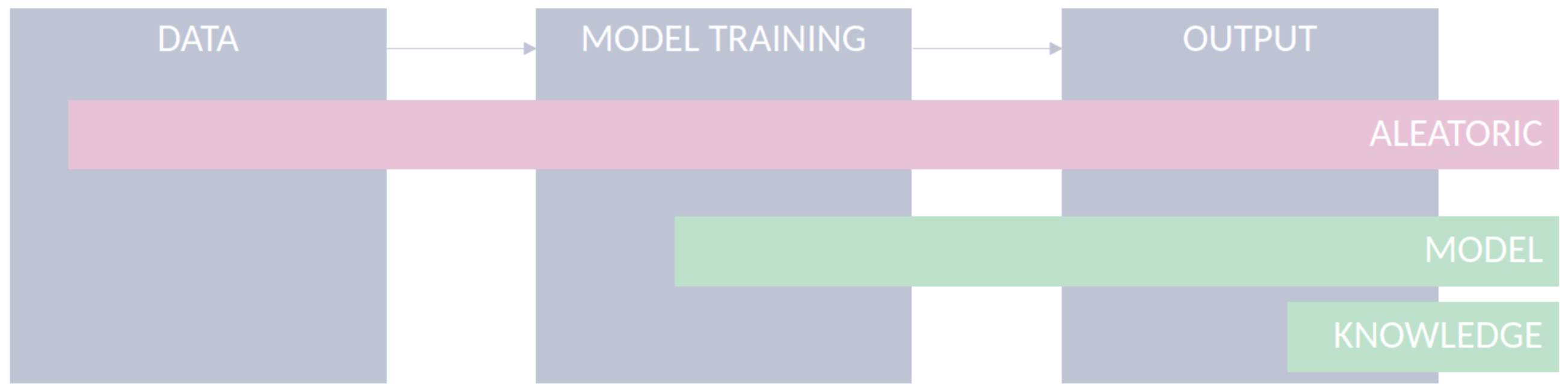
ML systems share a set of core components comprising data, an ML model, and its outputs. Uncertainties are present in all ML components under different sources, as visualized in Figure 1.
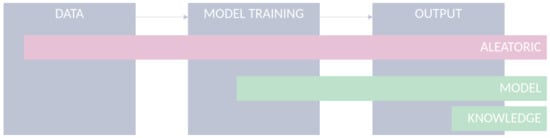
Figure 1.
Uncertainty in ml classification settings.
- Data: Data used to feed ML models are limited in their accuracy and potentially affected by various kinds of quality issues, which limits the models from being applied under optimal conditions [34,35]. For example, the uncertainty caused due to errors in the measurement might affect the performance of a given classification task. Although the aleatoric uncertainty is supposed to be irreducible for a specific dataset, incorporating additional features or improving the quality of the existing features can assist in its reduction [36];
- Model: For a given classification task, several ML models can be applied and developed. The choice of a model is arguably important and is often based on the degree of error in the model’s outcomes. However, besides models’ accuracy, the use of uncertainty quantification methods during model development can provide important elements to choose the right model for the problem at hand. Moreover, understanding the model’s uncertainty during training can give us insights about the specific limitations of each model and help in developing more robust models. The estimation of model uncertainty increases model interpretability, by allowing the user to interpret how confident the model is for a given prediction;
- Output: After the model’s training, estimating and quantifying uncertainty in a transductive way, in the sense of tailoring it to individual instances, are arguably relevant, all the more in safety-critical applications. For instance, in the context of computer-aided diagnosis systems, a prediction with high uncertainty shall justify either disregarding its output or conducting further medical examinations of the patient. In the latter, the goal is to retrieve additional evidence that supports or contradicts a given hypothesis. In the former, it is the case of classification with rejection, which is a viable option, where the presence and cost of errors can be detrimental to the performance of automated classification systems [33].
To illustrate the different sources of uncertainty and the methods for UQ, we introduce a scenario using a simulated small dataset shown in Figure 2. The scenario consists of a two-dimensional dataset with two classes, where features from class A were modeled with an unimodal Gaussian distribution and features from class B were modeled as a bimodal distribution with a mixture of two Gaussian distributions with highly unequal mass. The minor mode is approximately 5.5% of the mass of the major mode.
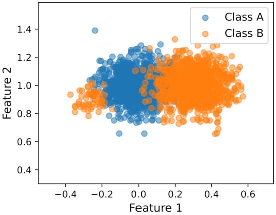
Figure 2.
Synthetic dataset used to illustrate the different sources of uncertainty in a toy scenario.
For model training, a Naive Bayes (NB) classifier using KDE was applied using a bootstrap approach with 50 bootstrap samples to estimate the sampling distribution of arbitrary functions of a dataset. Using this approach, it is possible to access the amount that a prediction changes when the model is fit on slightly different data.
The selected uncertainty quantification methods for each source of uncertainty were the following:
- Aleatoric uncertainty: The (Shannon) entropy is the most notable measure of uncertainty for probability distributions being more akin to aleatoric uncertainty. Equation (4), which measures the aleatoric uncertainty in terms of expectation over the entropies of distributions, was used for the rest of the analysis;
- Model uncertainty: Variation ratios (Equation (7)) were selected as a primary uncertainty quantification method, to estimate model uncertainty, as we were interested in evaluating the quality of the model fit. In this sense, changes in the predicted label have a significant impact on the variation ratio measure. Contrarily, measures based on entropies (Equation (6) is commonly used) can also be used, but the impact on the measure is lower, since in variation ratios, we are merely counting changes in the predictions, and in entropy measures, we are averaging the prediction probabilities [21];
- Knowledge uncertainty: Although the majority of works addressed the quantification of knowledge uncertainty with measures such as the mutual information using ensembles (Equation (6)), we argue that these kinds of measures are more akin to model uncertainty. The uncertainty related to the lack of data might be poorly modeled by these measures. In this perspective, we considered density estimation methods, commonly used for outlier or novelty detection, more prone to model knowledge uncertainty. Thus, the KUE measure (Equation (9)) was used to model knowledge uncertainty.
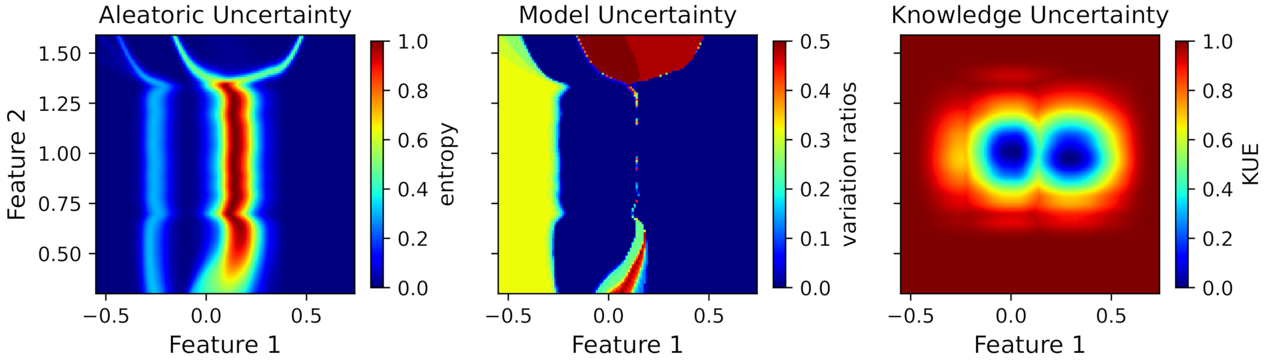
In order to visualize the uncertainty estimations in the whole region presented in Figure 2, we applied the uncertainty quantification measures to a new set of points that included all combinations of feature values in the defined region. Figure 3 shows the uncertainty values for each point of the feature space.
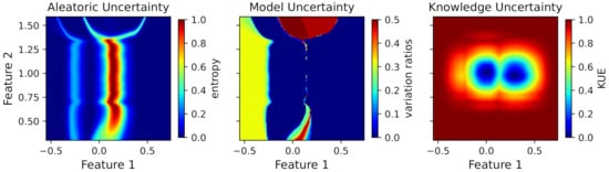
Figure 3.
Toy dataset uncertainty measures for aleatoric, model, and knowledge uncertainty (from left to right).
Observing the uncertainty regions for each source of uncertainty, one can see completely different behaviors depending on the uncertainty. The aleatoric uncertainty is high in the middle of the two major clusters (Feature 1 equals to 0.15 approximately), due to the overlap between the classes. The overlap between the cluster of class A and the minor cluster of class B also presents a higher uncertainty compared to the rest of the region. However, it does not produce an uncertainty as high as the overlap between the two major clusters due to the differences in the masses of both clusters. The entropy value is normalized to the maximum entropy, i.e., the logarithm of the number of classes.
Regarding the model uncertainty and referring to this toy scenario with two classes, the maximum possible value occurs when the frequency of both classes is equal, i.e., the variation ratios have a value of 0.5. The regions with higher uncertainty values are the ones with little evidence, since the model fit in these regions is highly dependent on the available data. Therefore, it is expected that slight differences in the training data, especially in regions with little evidence, have a high impact on the model fit and produce high model uncertainty. Observing the figure, it is possible to see that the minor cluster of class B produces a high model uncertainty. Additionally, the upper and lower regions between the major clusters also produce a high uncertainty, due to slight differences in the decision boundary on different bootstrap samples.
Finally, knowledge uncertainty was modeled using the feature density on the training data, which produces a high uncertainty in all the feature space without data.
For the classification with rejection, we define a rejection rule for each type of uncertainty, using the previously uncertainty measures to define the confidence threshold. The problem of choosing the optimal rejection point is not trivial and was not addressed in this work. There are several works entirely dedicated to this topic, such as the work of Condessa et al. [33] and Fisher et al. [37].
In our classification setting, the final prediction is given by the following rejection rule:
where is the classifier without rejection and is a function on the input that evaluates the uncertainty of the prediction model. This uncertainty function is given by the set of uncertainties—aleatoric (a), model (m), and knowledge (k)—through the following equation:
where is the set of available uncertainties, is an uncertainty function that evaluates uncertainty u, and is a threshold for the rejection point for uncertainty u.
Regarding aleatoric uncertainty, is equal to Equation (4) and the optimal threshold, , was obtained using the following equation:
where is a threshold in the interval , representing a normalized entropy value measured with Equation (4), and b is a rejection cost, here set to 0.5. For and , the notation from Section 2.2 was used, and the subsets represent the true rejections and false rejections using threshold , respectively.
The uncertainty function used for model uncertainty, , is equal to Equation (7), and was set to zero, which means that a prediction must be equal in all bootstraps samples to not be rejected. This assumption was made because if a sample is predicted differently using slightly different datasets, the model in that particular region will still have some uncertainty associated.
For knowledge uncertainty, is equal to Equation (9). To define , we used a 95% value of the training uncertainty values, meaning that . A detailed description of this approach is available in [24].
In summary, our proposed approach was developed in the context of classification with rejection where rejection was obtained through measures of uncertainty. These uncertainty measures were distinguished by three different sources: aleatoric, model, and knowledge uncertainty. For the uncertainty quantification, we used an entropy measure for aleatoric uncertainty (Equation (4)), the variation ratio measure for model uncertainty (Equation (7)), and KUE to quantify the knowledge uncertainty. Regarding the rejection setting, we applied the rejection rule from Equation (13), where each source of uncertainty has an uncertainty function given by Equation (14). For the training procedure, a bootstrap approach with 20 bootstrap samples was used, and the uncertainty measures were calculated. The evaluation of the selected models was performed through the accuracy and the nonrejection accuracy followed by the rejection fraction for each individual measure and also the total rejection fraction. In the case of the models’ combination, the performance measures from Equations (10)–(12) were also employed.
4. Experiments
In this section, we demonstrate the usefulness of uncertainty quantification using synthetic datasets and a benchmark dataset from the University of California Irvine (UCI) ML repository [38]. Specifically, we answer the following questions:
- Q1. How can UQ contribute to choosing the most suitable model for a given classification task?
- Q2. Can UQ be use to combine different models?
- Q3. Can visualization techniques improve UQ’s interpretability?
4.1. Analysis on Synthetic Data
Predicted uncertainties are often evaluated indirectly, since normally, data do not contain information about any sort of “ground truth” uncertainties. For this reason, the use of a synthetic dataset can more easily provide an intuition about the different types of uncertainties and their quantification. Furthermore, in a controllable setting, we can alter the size of the datasets, evaluate the models’ performance and uncertainties in different conditions, and introduce noise in the data to check the models’ robustness.
4.1.1. Uncertainty for Model Selection (Q1)
To answer Q1, we generated a dataset composed of a total of 150,000 ten-dimensional points corresponding to six different classes equally distributed. Features from each class were modeled using Gaussian, exponential, and uniform distributions. The distributions were randomly selected and could be unimodal or bimodal distributions. To evaluate the behavior of uncertainty estimations with the increasing number of training samples, the models were trained for different training sizes using a k-fold cross-validation as the validation strategy where k was set to 5. An exponential growth of the training samples was applied, starting with 50 samples per class (training size equals 300 samples).
For model training, different classifiers using a training size of 7692 samples were tested as presented in Table 1. Since features data were simulated using Gaussian, exponential, and uniform distributions, a focus on Bayesian models using Gaussian, KDE, and exponential distributions was employed. As expected, Bayesian models obtained higher baseline accuracies than the other tested classifiers, since part of the features likelihood was modeled with the true data distribution. With the purpose of answering Q1, the three classifiers highlighted in Table 1, with a similar baseline accuracy, were selected to continue the analysis. These classifiers were: (1) the NB classifier where the features likelihood was assumed to be Gaussian; (2) the NB classifier where the features likelihood was assumed to be exponential; (3) the Bayes classifier where the features likelihood was based on KDE. Additionally, the selected classifiers were trained using a bootstrap procedure with 20 bootstrap samples.

Table 1.
Performance measures (mean ± standard deviation) for different models using a training size of 7692 samples. The highlighted baseline accuracies represent the selected models that were considered for further analysis, since the models attained similar accuracy values.
For this analysis, only aleatoric and model uncertainty measures were considered, since a synthetic dataset without outliers was used. Therefore, KUE would be near zero and would not bring relevant information for this analysis.
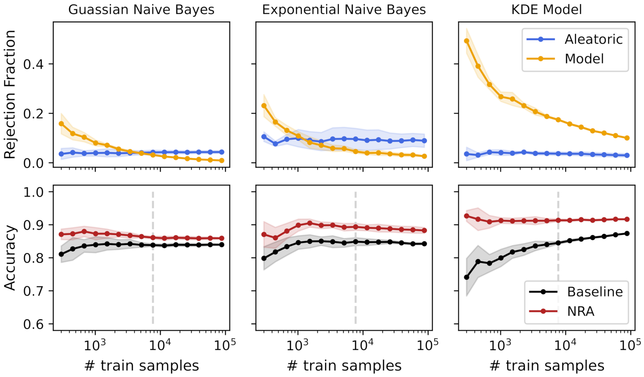
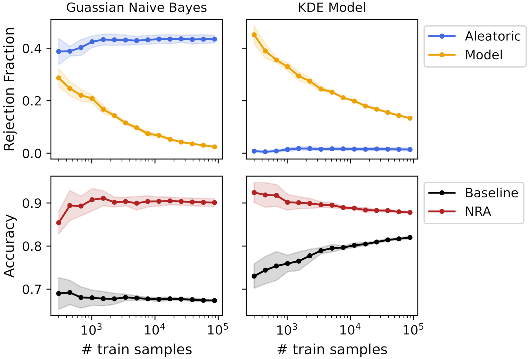
Figure 4 shows the rejection fraction and accuracy with the increasing number of training samples for the different tested models. The rejection fraction was obtained using both aleatoric and model uncertainty measures independently, and the nonrejected accuracy was obtained by rejecting all samples with aleatoric and/or model uncertainty (see Equation (13)).
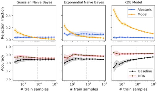
Figure 4.
Uncertainties’ rejection fraction and obtained accuracies using a k-fold cross-validation with an increasing number of training samples for 3 different models. The vertical line represents a training size that obtained a similar baseline accuracy for all models.
As previously mentioned, the model’s accuracy is often one of the most important elements to model selection. However, we argue that uncertainty quantification methods should also be evaluated during the model’s training, to help us choose the right model. Observing Figure 4, different models can achieve the same accuracy, but with different degrees of uncertainty. For example, for a training size of 7692 samples (dashed gray line in Figure 4), the three models obtained a baseline accuracy of 84%, approximately. Seen only from this point of view, the decision between the three models would be equal. However, observing the rejection fraction from uncertainty measures, it is easy to understand that the KDE model had higher model uncertainty compared with the other two models. The reason for this difference is that the KDE model is more complex, which means that it needs more data to correctly model the data distribution. Therefore, the differences in the bootstrap samples have a high impact on the model fit, meaning that the same sample is classified differently depending on the bootstrap sample used to fit the model. Additionally, observing the standard deviation with the increasing number of training samples, we can note a slight decrease in both the rejection fraction and accuracy values, except from the exponential model, which seemed to have an almost constant value across the different training sizes. Using this information and since the accuracy was approximately equal for the three models, the choice of a Gaussian NB would be probably preferable due to its low aleatoric and model uncertainty.
Nonetheless, if the rejection of samples or the addition of new samples is an option, a different analysis can be performed. By definition, aleatoric uncertainty is irreducible for the same dataset, which was verified with these experimental results. Increasing the number of training samples did not change the aleatoric uncertainty, making the rejection fraction mostly constant across the different training sizes. Contrarily, model uncertainty decreased with the increase of the number of training samples, tending towards zero when the model fit was equal for all bootstrap samples. Thus, the analysis of model uncertainty can give us insights about the usefulness of adding more samples for the model’s training. In Gaussian and KDE models, the decrease of model uncertainty had a clear increase in the baseline accuracy. For the Gaussian NB model, from training samples, the baseline accuracy was mostly constant and the decrease of model uncertainty was not significant. This means that the model fit did not change using different bootstrap samples, and the addition of new data did not improve the model’s performance. However, observing the KDE model, due to its high rejection fraction of model uncertainty, the addition of new samples still increased the model’s performance. Furthermore, the nonrejected accuracy was always higher than the baseline accuracy, and it was mostly constant across the different training sizes. This means that the model uncertainty measure was in fact detecting the regions in the feature space responsible for a high number of misclassifications due to a poor model fit.
4.1.2. Uncertainty for Models’ Combination (Q2)
From the analysis of the previous question, we observed that different models had different degrees of uncertainty for the same training size. Since different models were based on different assumptions, we hypothesized that uncertainty measures can be used to combine different models, producing a more robust model. In order to validate this hypothesis, a new dataset composed of 150,000 ten-dimensional points corresponding to six different classes equally distributed and modeled as a bimodal Gaussian distribution was generated.
A Gaussian NB and a KDE Bayes classifier were trained with a bootstrap approach with 20 bootstrap samples. Figure 5 shows the rejection fraction and accuracy with the increasing number of training samples for both models. As the Gaussian model uses unimodal distributions to fit the features data and the dataset was composed of features modeled as bimodal Gaussian distributions, the Gaussian NB classifier presented a high rejection fraction due to aleatoric uncertainty, since the overlap between the fit distributions was high. Contrarily, the KDE Bayes classifier deals well with bimodal distributions, which resulted in a low overlap between classes, obtaining a low rejection fraction due to aleatoric uncertainty. Regarding model uncertainty, although both models started with a high rejection fraction, the Gaussian NB reached training samples with almost zero rejection, and the KDE model, due to its complexity, still had a 10% rejection rate, approximately. In summary, the Gaussian NB had high aleatoric uncertainty and low model uncertainty, and the KDE Bayes classifier had low aleatoric uncertainty and high model uncertainty.

Figure 5.
Uncertainties’ rejection fraction and obtained accuracies using a k-fold cross-validation with an increasing number of training samples for Gaussian NB and KDE Bayes models.
To verify the potential for combining both models using uncertainty measures, the following combination rules were applied:
where and represent the Gaussian NB and KDE Bayes classifier and is the uncertainty function defined in Equation (14).
To validate that the proposed combination strategy performed better than the individual models, we applied the performance measures proposed in the work of Condessa et al. [33]. To compare the performance of the classifiers with rejection, 10% of the rejected samples were used with the highest training size available (∼90,000 training samples).
In Table 2, the obtained results for the three models using a 10% rejection fraction are shown. The combination strategy using the uncertainties of both individual models resulted in higher values for the three performance measures for classifiers with rejection, namely the nonrejected accuracy, classification quality, and rejection quality.
Table 2.
Performance measures for individual models (Gaussian naive Bayes and KDE Bayes) and a combination of both models. The results were obtained using a rejection fraction of 10% and a training size of 90,000 samples.
These preliminary results showed that the access to uncertainty estimations during the model’s development might be a useful source of information to develop more robust models. Although a simpler model, such as an NB classifier, can have a lower performance in comparison with more complex models, the use of uncertainty estimations can provide information about the specific regions where the model has low uncertainty. Using this information in combination with more powerful models can in fact increase the overall model performance.
4.1.3. Uncertainty Visualization (Q3)
To use ML in high-stakes applications, we need auditing tools to build confidence in the models and their decisions. Besides quantification metrics, visualization techniques have been used to support the interpretability of classification models. Therefore, to answer this question, we quantified the different sources of uncertainty using visualization methods to assist in interpreting the models’ uncertainty during model development and also to audit a given decision.
For uncertainty visualization, the dataset from Section 4.1.2 with a training size of was used. To simulate a realistic real-world setting, some outliers were added to the test set. These outliers were generated from a Gaussian distribution that had a covariance matrix that is four-times larger than that of the dataset itself. Fifty outliers per class were generated, resulting in a total of 300 outliers.
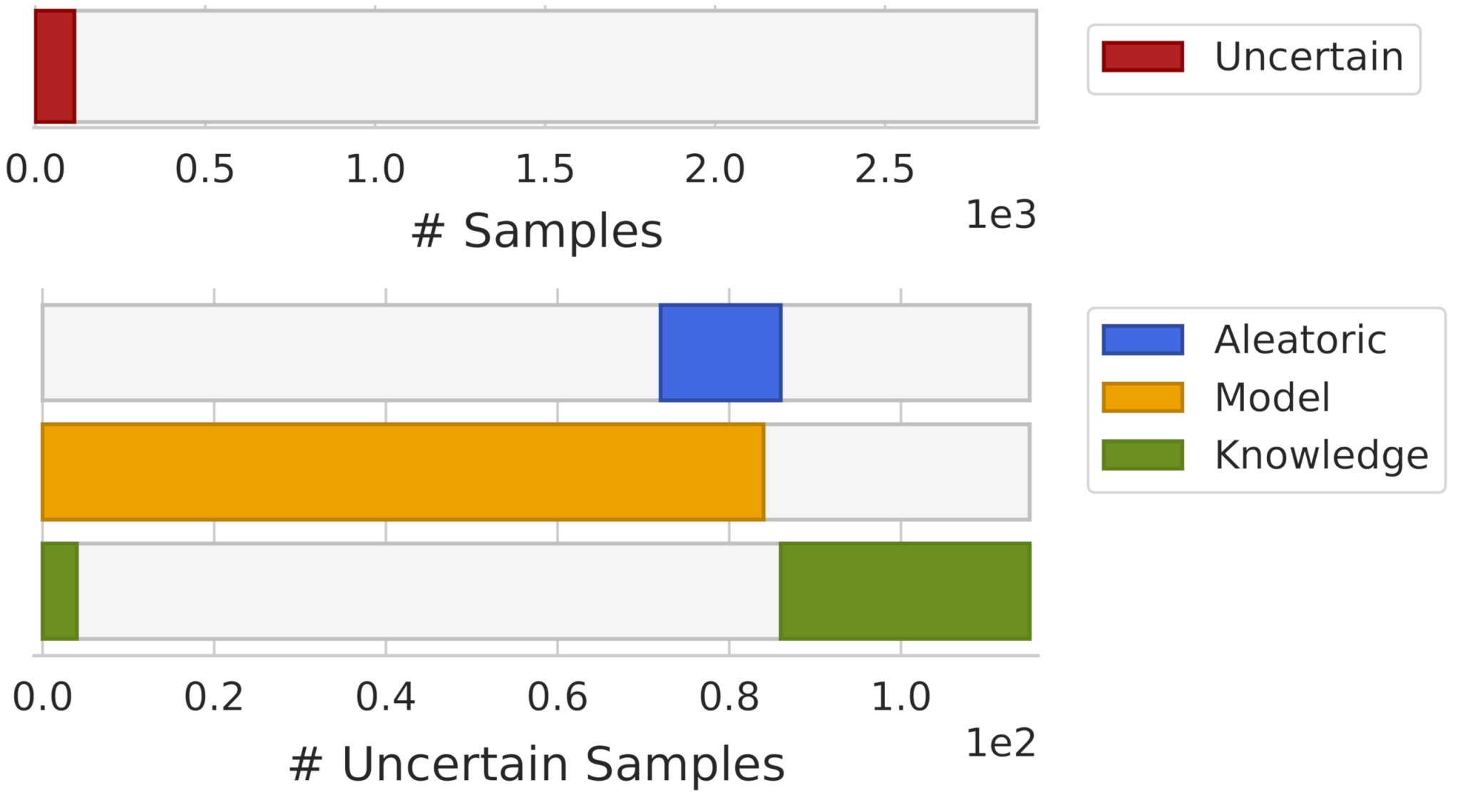
In Figure 6, an overview of the uncertainty estimation obtained during the model’s development is shown. In this visualization, the x-axis represents the number of samples where samples are ordered by uncertainty. Using this ordering scheme, it was possible to interpret the overall dataset uncertainty (upper bar), as well as the proportion of the different sources of uncertainty across the dataset (lower bars). The size of each bar represents the number of samples rejected by each type of uncertainty. Furthermore, this visualization allowed us to make some observations, such as noting that all rejected samples by model uncertainty were also rejected by aleatoric uncertainty.
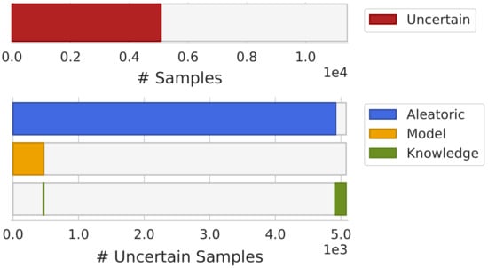
Figure 6.
Overview of the overall dataset uncertainty (upper bar) and uncertainties distribution by the uncertainty source (lower bars).
Similarly, this representation can be applied to each individual class. Analyzing the uncertainty by each class can give us insights about the particular limitations of the model being used. Figure 7 presents the obtained uncertainty by uncertainty source and class. Note that almost all samples with knowledge uncertainty from Figure 6 were the generated outliers and do not have a representation in Figure 7.
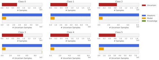
Figure 7.
Uncertainty distribution by uncertainty source and class.
Besides the visualization applied to the overall classifier’s uncertainty, an alternative is to audit the reliability of a given prediction, answering questions such as: Can I trust this prediction? Why did I reject this sample?
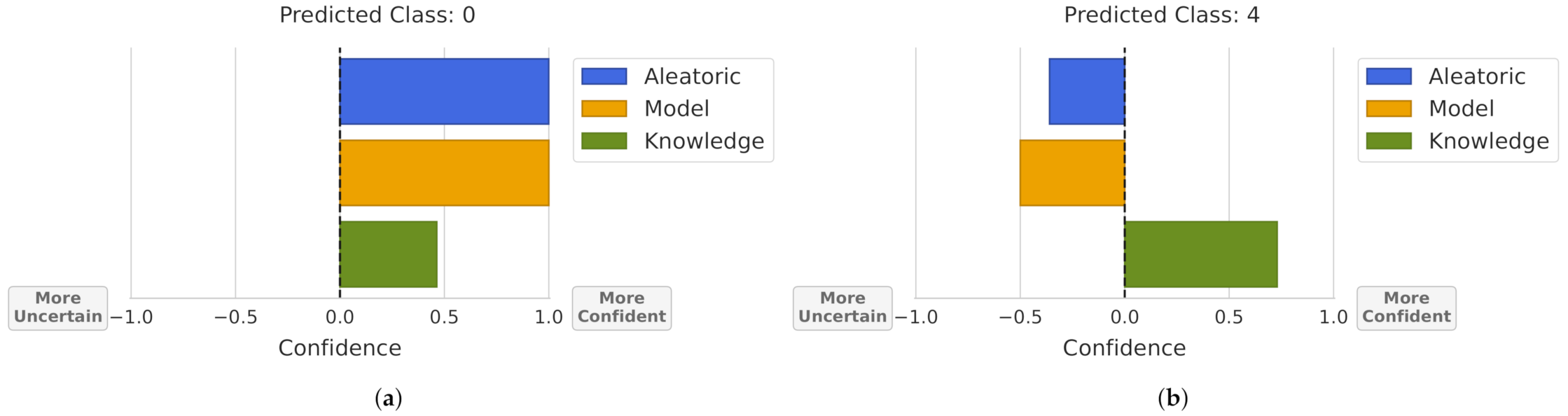
For this purpose, using the uncertainty estimations for each type of uncertainty, Figure 8 was obtained. In this visualization, the bar’s size represents how much the model is confident or uncertain about a prediction by uncertainty type. To make the visualization more intuitive, 0 confidence/uncertainty represents the obtained threshold for rejecting a sample. Then, the bars’ sizes where normalized between 0 and 1 by the maximum/minimum theoretical value for each uncertainty.

Figure 8.
Prediction uncertainty. A confidence value of 0 represents the obtained threshold for rejecting a sample by the uncertainty source. Bars’ sizes are normalized between the maximum theoretical confidence/uncertainty. (a) Prediction not rejected by all uncertainty sources. (b) Prediction rejected by aleatoric and model uncertainty.
Note that, in the aleatoric uncertainty, we visualize the prediction’s expected data entropy, meaning that in Figure 8a, the prediction probability was near 100% (entropy of 0). In the case of Figure 8b, the obtained entropy was greater than the defined threshold for rejection and its value represents approximately 1/3 of the entropies that range between 1 and the rejection threshold. In the case of model uncertainty, we evaluated if a given prediction changes between different bootstrap samples, i.e., the bar’s size represents the normalized variation ratios. In Figure 8a, the prediction was the same in all bootstrap samples, obtaining a maximum confidence value, and in Figure 8b, the prediction changed half the total number of possibilities, which are given by the number of bootstrap samples and the number of classes. For instance, this dataset had 6 classes and 20 bootstrap samples were used, meaning that the maximum variation ratio was 0.8, and the prediction from Figure 8b obtained a variation ratio of 0.4. Finally, the knowledge uncertainty represents how much a prediction is similar to the training dataset, in terms of probability density. Thus, Figure 8a represents a prediction where the combination of the features density resulted in a KDE value close to the rejection threshold, i.e., few training samples were similar to this prediction. In the case of Figure 8b, the sample was more similar to the samples in the training dataset.
4.2. Experiments on a Human Activity Recognition Dataset
In order to broaden our analysis, we conducted an additional experiment with a benchmark dataset from the UCI repository [38]. As a case study, we selected a har dataset [39] that contains six classes (walking, walking upstairs, walking downstairs, sitting, standing, and laying), recorded with the accelerometer and gyroscope smartphone sensors. Besides the importance of UQ for trustworthy ML systems, the use of uncertainty measures for human movements analysis plays also an important role in the recognition of abnormal human activities or the analysis, diagnosis, and monitoring of neurodegenerative conditions [40]. Furthermore, the high number of available samples (10,299 samples) in this dataset allowed us to make a similar evaluation to the synthetic data. For the data split into training and test sets, we used the available partition in the repository, where 70% of the volunteers were selected for generating the training data and 30% the test data. Regarding the feature vector, the original 561-feature vector with time and frequency domain variables was reduced using features correlation and the sequential forward feature selector, resulting in a 17-dimensional feature vector.
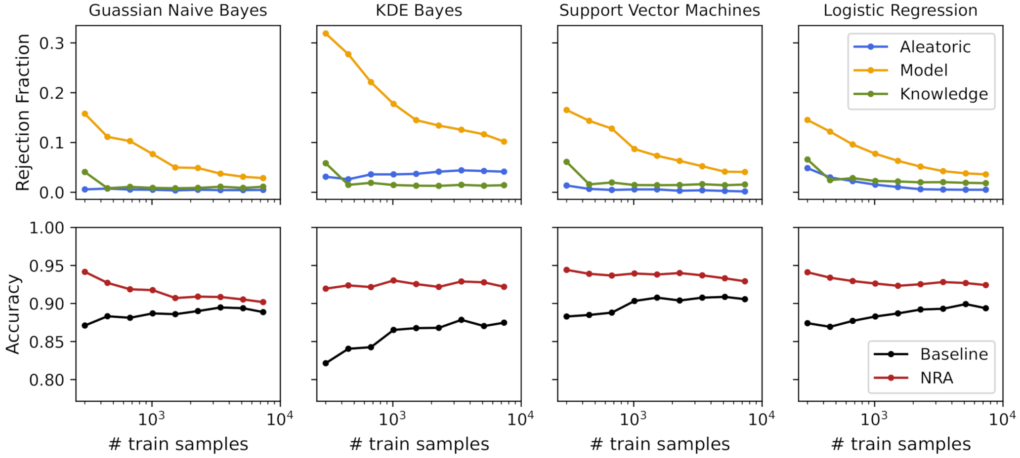
Similar to Section 4.1.1, we applied a training size exponential growth, starting with 300 samples (50 per class) until the maximum training size of 7352 samples. For model training, we tested different classifiers with 20 bootstrap samples. Table 3 shows the obtained baseline accuracy, as well as the nonrejected accuracy and the rejection fraction for each of the tested classifiers. To visualize the behavior of accuracy and the corresponding rejection fraction for each type of uncertainty, we selected the 4 models that obtained higher baseline accuracy. Figure 9 shows these performance measures with the increased number of samples used to train the classifiers.
Table 3.
Performance measures for different models using a training size of 7352 samples and the har dataset.
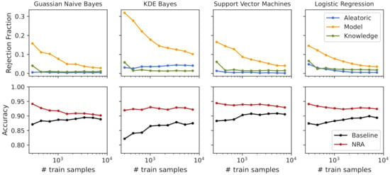
Figure 9.
Uncertainties’ rejection fraction and obtained accuracies with the increasing number of training samples for the har dataset.
For the HAR dataset, the rejection fraction obtained with both the aleatoric and knowledge uncertainty measures presented a low value for all training sizes and classifiers being analyzed. As expected, regarding the model uncertainty, the rejection fraction decreased with the increasing number of training samples for all classifiers, where more complex classifiers had a higher rejection fraction than simpler classifiers. Due to the low obtained uncertainty (rejection fraction < 4%) and satisfactory accuracy (baseline accuracy of 89%), the Gaussian NB classifier was selected.
Using the visualization scheme presented in Section 4.1.3, Figure 10 shows the overall dataset uncertainty and the uncertainty type distribution across the uncertain samples. Although only 4% of the test samples were rejected, we can make some observations about the uncertain samples. The majority of uncertain samples rejected by aleatoric uncertainty were also rejected by model uncertainty. Regions with an overlap between classes (aleatoric uncertainty) were also regions where it was expected that the model fit would change between bootstrap samples. In the case of knowledge uncertainty, it was expected that samples with knowledge uncertainty would not have aleatoric uncertainty. However, for model uncertainty, it is possible that some samples shared both model and knowledge uncertainty, which is also verified with Figure 10.
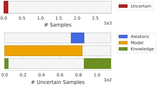
Figure 10.
HAR dataset uncertainty overview.
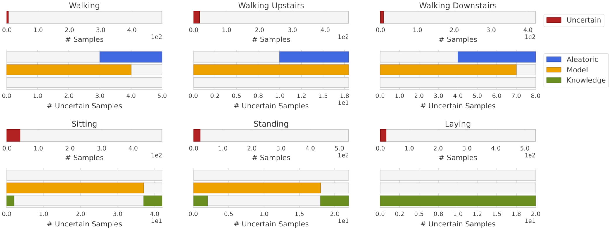
Figure 11 shows the uncertainty distribution by class. From it, we can conclude that aleatoric uncertainty was presented only in walking, walking upstairs and walking downstairs, which makes perfect sense due to the similarity of these three classes. It is also possible to note that laying class did not have aleatoric or model uncertainty. However, it was the class with the highest knowledge uncertainty. Both sitting and standing classes had a similar pattern in terms of uncertainty, where the sitting class was the one with the highest number of uncertain samples.

Figure 11.
HAR dataset uncertainty overview by class.
To validate the combination strategy proposed in Section 4.1.2 using a real dataset, we decided to combine the two models with lower accuracy and higher uncertainty. Thus, the KDE Bayes model and logistic regression were combined for the different training sizes. To compare the performance of classifiers with rejection, we needed to ensure the same rejection fraction for the three classifiers. Thus, the obtained rejection fraction for the models’ combination, given by Equation (16), was employed for both the KDE Bayes and logistic regression classifiers. Figure 12 shows the performance measures for classification with rejection for the individual models and their combination. Observing the results, we can conclude that the combination strategy outperformed the individual classifiers for almost all training sizes and performance measures. It is also interesting to note that the combination strategy resulted always in a lower rejection fraction than the obtained rejection fraction for the individual classifiers, which can be confirmed by analyzing Figure 9 and Figure 12.
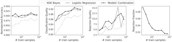
Figure 12.
Performance measures for classification with rejection for different training sizes.
5. Conclusions
As ML models are increasingly being integrated into safety-critical applications, incorporating uncertainty quantification estimates should become a required part of the ML methodology. Uncertainty quantification can be used for “uncertainty-informed” decisions and to support developers and end-users by increasing the interpretability of and trust in model predictions.
We introduced a complete study focused on how uncertainty quantification can be used in practice through three research questions: (1) How can UQ contribute to choosing the most suitable model for a given classification task? (2) Can UQ be used to combine different models in a principled manner? (3) Can visualization techniques improve UQ’s interpretability? These questions were answered using a synthetic dataset and a HAR dataset from the UCI repository.
Regarding the first question, we showed that uncertainty quantification in combination with the model’s accuracy can give us important elements to choose the most suitable model. For instance, the decision between different classifiers with the same accuracy can benefit from the uncertainty quantification methods, whereas classifiers with lower degrees of uncertainty can be preferable. Furthermore, if model uncertainty is high and the addition of new samples is possible, the increase of training samples can reduce the model uncertainty and consequently increase the model’s accuracy. By using uncertainty as a complement of performance measures, we can make more informed decisions in model selection. In future work, we will explore how the UQ measures can be used in the context of active learning. Active learning is the subset of ML in which the learning algorithm queries users to label training data. The choice of the samples to be labeled is achieved through measures that rank samples based on their potential informativeness. Alternative or complementary ranking measures based on uncertainty can be explored.
Based on two models with different degrees of uncertainty, we proposed a naive uncertainty combination approach for models’ combination to answer the second question. The preliminary results showed that the combination strategy outperformed the individual models. Although the proposed naive approach achieved good results, the combination strategy presented some limitations for its application in a scenario with more than two models. A more versatile combination that considers the possibility of adding more models and uses their degree of uncertainty must be developed. Therefore, for future work, we will explore more comprehensive model combination methods to address more complex problems.
In the third question, we explored visualization techniques to assist in interpreting classifiers’ uncertainty during the model’s development and also to audit a given decision. Understanding which type of uncertainty is present during the model’s development can give us insights into the limitations of each model and allow us to take actions in accordance. In the context of prediction reliability, the proposed visualization techniques were used to access the interpretability of the rejection option in which a rejection may correspond to a low prediction probability (aleatoric uncertainty), a poor model fit (model uncertainty), or an outlier (knowledge uncertainty). As a limitation of our study, we identify that an individual rejection threshold for each source of uncertainty may not be a reliable solution for every ML problem. Defining the best rejection threshold is still an open challenge. Our future research on this topic will focus on understanding how optimization techniques can be used to establish the most adequate rejection thresholds, either individually or by unifying the three quantification measures.
We hope this paper might spark future research on how to consider uncertainty quantification as a tool to improve the ML model development lifecycle.
Author Contributions
Conceptualization, M.B. and H.G.; methodology, M.B., D.F. and H.G.; software, M.B.; validation, M.B., D.F. and H.G.; investigation, M.B., D.F., R.S. (Ricardo Santos), R.S. (Raquel Simão) and H.G.; writing—original draft preparation, M.B. and D.F.; writing—review and editing, M.B., D.F., R.S. (Ricardo Santos), R.S. (Raquel Simão) and H.G.; visualization, R.S. (Ricardo Santos) and M.B.; supervision, H.G. All authors have read and agreed to the published version of the manuscript.
Funding
This research was financially supported by the project Geolocation non-Assisted by GPS for Mobile Networks in Indoor and Outdoor Environment (GARMIO), co-funded by Portugal 2020, framed under the COMPETE 2020 (Operational Programme Competitiveness and Internationalization) and European Regional Development Fund (ERDF) from European Union (EU), with Operation Code POCI-01-0247-FEDER-033479.
Institutional Review Board Statement
Not applicable.
Informed Consent Statement
Not applicable.
Data Availability Statement
Publicly available datasets were analyzed in this study. These data can be found at the UC Irvine Machine Learning Repository, available at https://archive.ics.uci.edu/ml/datasets/human+activity+recognition+using+smartphones (accessed on 20 December 2021).
Conflicts of Interest
The authors declare no conflict of interest.
References
- Cobb, A.D.; Jalaian, B.; Bastian, N.D.; Russell, S. Toward Safe Decision-Making via Uncertainty Quantification in Machine Learning. In Systems Engineering and Artificial Intelligence; Springer: Berlin/Heidelberg, Germany, 2021; pp. 379–399. [Google Scholar]
- Senge, R.; Bösner, S.; Dembczyński, K.; Haasenritter, J.; Hirsch, O.; Donner-Banzhoff, N.; Hüllermeier, E. Reliable classification: Learning classifiers that distinguish aleatoric and epistemic uncertainty. Inf. Sci. 2014, 255, 16–29. [Google Scholar] [CrossRef] [Green Version]
- Kompa, B.; Snoek, J.; Beam, A.L. Second opinion needed: Communicating uncertainty in medical machine learning. NPJ Digit. Med. 2021, 4, 1–6. [Google Scholar] [CrossRef] [PubMed]
- Hüllermeier, E.; Waegeman, W. Aleatoric and epistemic uncertainty in machine learning: An introduction to concepts and methods. Mach. Learn. 2021, 110, 457–506. [Google Scholar] [CrossRef]
- Huang, Z.; Lam, H.; Zhang, H. Quantifying Epistemic Uncertainty in Deep Learning. arXiv 2021, arXiv:2110.12122. [Google Scholar]
- Holzinger, A.; Langs, G.; Denk, H.; Zatloukal, K.; Müller, H. Causability and explainability of artificial intelligence in medicine. Wiley Interdiscip. Rev. Data Min. Knowl. Discov. 2019, 9, e1312. [Google Scholar] [CrossRef] [PubMed] [Green Version]
- Nguyen, V.L.; Shaker, M.H.; Hüllermeier, E. How to measure uncertainty in uncertainty sampling for active learning. Mach. Learn. 2021, 1–34. [Google Scholar] [CrossRef]
- Bota, P.; Silva, J.; Folgado, D.; Gamboa, H. A semi-automatic annotation approach for human activity recognition. Sensors 2019, 19, 501. [Google Scholar] [CrossRef] [PubMed] [Green Version]
- Ghosh, S.; Liao, Q.V.; Ramamurthy, K.N.; Navratil, J.; Sattigeri, P.; Varshney, K.R.; Zhang, Y. Uncertainty Quantification 360: A Holistic Toolkit for Quantifying and Communicating the Uncertainty of AI. arXiv 2021, arXiv:2106.01410. [Google Scholar]
- Chung, Y.; Char, I.; Guo, H.; Schneider, J.; Neiswanger, W. Uncertainty toolbox: An open-source library for assessing, visualizing, and improving uncertainty quantification. arXiv 2021, arXiv:2109.10254. [Google Scholar]
- Oala, L.; Murchison, A.G.; Balachandran, P.; Choudhary, S.; Fehr, J.; Leite, A.W.; Goldschmidt, P.G.; Johner, C.; Schörverth, E.D.; Nakasi, R.; et al. Machine Learning for Health: Algorithm Auditing & Quality Control. J. Med. Syst. 2021, 45, 1–8. [Google Scholar]
- Bosnić, Z.; Kononenko, I. An overview of advances in reliability estimation of individual predictions in machine learning. Intell. Data Anal. 2009, 13, 385–401. [Google Scholar] [CrossRef] [Green Version]
- Tornede, A.; Gehring, L.; Tornede, T.; Wever, M.; Hüllermeier, E. Algorithm selection on a meta level. arXiv 2021, arXiv:2107.09414. [Google Scholar]
- Neto, M.P.; Paulovich, F.V. Explainable Matrix-Visualization for Global and Local Interpretability of Random Forest Classification Ensembles. IEEE Trans. Vis. Comput. Graph. 2020, 27, 1427–1437. [Google Scholar] [CrossRef] [PubMed]
- Shaker, M.H.; Hüllermeier, E. Ensemble-based Uncertainty Quantification: Bayesian versus Credal Inference. arXiv 2021, arXiv:2107.10384. [Google Scholar]
- Malinin, A.; Prokhorenkova, L.; Ustimenko, A. Uncertainty in gradient boosting via ensembles. arXiv 2020, arXiv:2006.10562. [Google Scholar]
- Depeweg, S.; Hernandez-Lobato, J.M.; Doshi-Velez, F.; Udluft, S. Decomposition of uncertainty in Bayesian deep learning for efficient and risk-sensitive learning. In Proceedings of the International Conference on Machine Learning, Stockholm, Sweden, 10–15 July 2018; pp. 1184–1193. [Google Scholar]
- Shaker, M.H.; Hüllermeier, E. Aleatoric and epistemic uncertainty with random forests. arXiv 2020, arXiv:2001.00893. [Google Scholar]
- Efron, B.; Tibshirani, R. Bootstrap methods for standard errors, confidence intervals, and other measures of statistical accuracy. Stat. Sci. 1986, 1, 54–75. [Google Scholar] [CrossRef]
- Stracuzzi, D.J.; Darling, M.C.; Peterson, M.G.; Chen, M.G. Quantifying Uncertainty to Improve Decision Making in Machine Learning; Technical Report; Sandia National Lab. (SNL-NM): Albuquerque, NM, USA, 2018.
- Mena, J.; Pujol, O.; Vitrià, J. Uncertainty-based rejection wrappers for black-box classifiers. IEEE Access 2020, 8, 101721–101746. [Google Scholar] [CrossRef]
- Geng, C.; Huang, S.j.; Chen, S. Recent advances in open set recognition: A survey. IEEE Trans. Pattern Anal. Mach. Intell. 2020, 43, 3614–3631. [Google Scholar] [CrossRef] [Green Version]
- Perello-Nieto, M.; Telmo De Menezes Filho, E.S.; Kull, M.; Flach, P. Background Check: A general technique to build more reliable and versatile classifiers. In Proceedings of the 2016 IEEE 16th International Conference on Data Mining (ICDM), Barcelona, Spain, 12–15 December 2016; pp. 1143–1148. [Google Scholar]
- Pires, C.; Barandas, M.; Fernandes, L.; Folgado, D.; Gamboa, H. Towards Knowledge Uncertainty Estimation for Open Set Recognition. Mach. Learn. Knowl. Extr. 2020, 2, 505–532. [Google Scholar] [CrossRef]
- Chow, C. On optimum recognition error and reject tradeoff. IEEE Trans. Inf. Theory 1970, 16, 41–46. [Google Scholar] [CrossRef] [Green Version]
- Tax, D.M.; Duin, R.P. Growing a multi-class classifier with a reject option. Pattern Recognit. Lett. 2008, 29, 1565–1570. [Google Scholar] [CrossRef]
- Fumera, G.; Roli, F.; Giacinto, G. Reject option with multiple thresholds. Pattern Recognit. 2000, 33, 2099–2101. [Google Scholar] [CrossRef]
- Hanczar, B. Performance visualization spaces for classification with rejection option. Pattern Recognit. 2019, 96, 106984. [Google Scholar] [CrossRef]
- Franc, V.; Prusa, D.; Voracek, V. Optimal strategies for reject option classifiers. arXiv 2021, arXiv:2101.12523. [Google Scholar]
- Charoenphakdee, N.; Cui, Z.; Zhang, Y.; Sugiyama, M. Classification with rejection based on cost-sensitive classification. In Proceedings of the International Conference on Machine Learning, Virtual, 13–15 April 2021; pp. 1507–1517. [Google Scholar]
- Gal, Y. Uncertainty in Deep Learning. Ph.D. Dissertation, University of Cambridge, Cambridge, UK, 2016. [Google Scholar]
- Nadeem, M.S.A.; Zucker, J.D.; Hanczar, B. Accuracy-rejection curves (ARCs) for comparing classification methods with a reject option. In Proceedings of the third International Workshop on Machine Learning in Systems Biology, Ljubljana, Slovenia, 5–6 September 2009; pp. 65–81. [Google Scholar]
- Condessa, F.; Bioucas-Dias, J.; Kovačević, J. Performance measures for classification systems with rejection. Pattern Recognit. 2017, 63, 437–450. [Google Scholar] [CrossRef] [Green Version]
- Kläs, M. Towards identifying and managing sources of uncertainty in AI and machine learning models-an overview. arXiv 2018, arXiv:1811.11669. [Google Scholar]
- Campagner, A.; Cabitza, F.; Ciucci, D. Three-way decision for handling uncertainty in machine learning: A narrative review. In International Joint Conference on Rough Sets; Springer: Berlin/Heidelberg, Germany, 2020; pp. 137–152. [Google Scholar]
- Sambyal, A.S.; Krishnan, N.C.; Bathula, D.R. Towards Reducing Aleatoric Uncertainty for Medical Imaging Tasks. arXiv 2021, arXiv:2110.11012. [Google Scholar]
- Fischer, L.; Hammer, B.; Wersing, H. Optimal local rejection for classifiers. Neurocomputing 2016, 214, 445–457. [Google Scholar] [CrossRef]
- Dua, D.; Graff, C. UCI Machine Learning Repository; University of California, School of Information and Computer Science: Irvine, CA, USA, 2019; Available online: http://archive.ics.uci.edu/ml (accessed on 20 December 2021).
- Anguita, D.; Ghio, A.; Oneto, L.; Parra, X.; Reyes-Ortiz, J.L. A public domain dataset for human activity recognition using smartphones. Esann 2013, 3, 3. [Google Scholar]
- Buckley, C.; Alcock, L.; McArdle, R.; Rehman, R.Z.U.; Del Din, S.; Mazzà, C.; Yarnall, A.J.; Rochester, L. The role of movement analysis in diagnosing and monitoring neurodegenerative conditions: Insights from gait and postural control. Brain Sci. 2019, 9, 34. [Google Scholar] [CrossRef] [PubMed] [Green Version]


Publisher’s Note: MDPI stays neutral with regard to jurisdictional claims in published maps and institutional affiliations. |
© 2022 by the authors. Licensee MDPI, Basel, Switzerland. This article is an open access article distributed under the terms and conditions of the Creative Commons Attribution (CC BY) license (https://creativecommons.org/licenses/by/4.0/).