1. Introduction
The expected reliability reduction [
1,
2] in digital FET-based nano-circuits will hardly be managed by the classical single-fault paradigm widely used in testing and in some fault-tolerant design techniques. In several applications, multiple faults cannot be neglected during the design, test and reliability assessment processes, and the problem is expected to worsen in the perspective successors of such technologies.
The need for design automation tools accounting for multiple faults may be satisfied by either probabilistic or deterministic techniques, according to the application: probabilistic techniques [
3] can estimate error probabilities, while deterministic ones can assess fault-tolerant capabilities with respect to given fault multiplicities.
In the deterministic case, Boolean proof engines have been successfully used in the synthesis, verification and testing of digital ICs. In the testing context, Boolean satisfiability (SAT) [
4] has been used in test generation [
5,
6] and fault diagnosis [
7,
8] for several kinds of fault models, mainly considering single faults. Recently, SAT-based test generation has been applied to the case of multiple faults in combinational logic modules, showing that test sequences featuring full coverage on single stuck-at faults need very few additional test vectors to achieve full coverage on multiple gate-output stuck-at faults as well [
9,
10].
SAT-based fault diagnosis for single and multiple faults typically uses additional variables to encode the set of possible faulty circuits. In this regard, two possibilities have been explored depending on whether such additional variables are used to encode specific faulty behaviors of a logic cell (such as those induced by stuck-ats or other kind of faults) or to simply encode fault locations in a fault model-free approach [
11].
In other cases, including fault-tolerant systems featuring either error detection or fault masking properties, the perspective is slightly different, but multiple faults still have to be accounted for. For instance, the error masking properties of a fault-tolerant system or the accuracy of an approximate computing circuit may have to be assessed with respect to a given fault cardinality. In such cases, it may be required to reason about circuit properties in the presence of multiple faults.
The approaches that consider specific fault models mainly work at a structural level: they inject faults in all logic cells of the fault-free circuit by using extra logic gates and additional signals, thus modeling the circuit in the possible presence of multiple faults; then, they derive a CNF (i.e., conjunctive normal form) from such a model.
On the contrary, the model-free approaches [
11] consider possible fault locations instead of specific faults. They can also directly modify the CNF representing the fault-free circuit by adding variables to the CNF that allow signals to assume values that are not consistent with the fault-free case.
In the case of a combinational circuit, the task of fault diagnosis is to find configurations of additional variables justifying a set of possibly erroneous output configurations as they are individuated by production testing. When analyzing the reliability of a circuit design, these techniques can be used to check whether multiple faults exist that produce output errors violating some required property.
In both cases, a huge set of additional variable assignments exists that satisfies the CNF of the circuit under diagnosis/reliability constraints. Therefore, cardinality constraints are necessary to achieve meaningful solutions. For instance, in [
11], given a set of input assignments and output responses, a Quantified Boolean Formula (QBF) is built over the CNF describing the possible faulty circuits and it is solved under cardinality constraints.
In this context, we first compare model-based (considering stuck-at faults) approaches with model-free ones and we discuss their limitations. Then, we extend the model-free approach used in [
11] in two ways. In the first one, we build the CNF describing the faulty circuits that account in a more realistic way for faults affecting logic cells while still avoiding structural modifications to the circuit. Then, a model is proposed that allows us to consider faults that cannot be accounted for by either existing structural or model-free fault injection techniques. In particular, these are faults affecting the circuit interconnections [
12] or internal bridging faults resulting in intermediate voltages at the outputs of gates [
13].
The problem of fault multiplicity is here approached using a Pseudo Boolean SAT solver/optimizer [
14] to minimize the number of additional variables to be set in order to satisfy a given condition on the output error. In different applications, instead, fault multiplicity can be constrained to be smaller than a given threshold, while using the Pseudo Boolean SAT solver/optimizer to maximize, for instance, the number of output errors or their numerical value (in arithmetic units). Finally, a simpler SAT solver [
15] can be used when optimization is not required.
The proposed method is not applied here to a specific problem of testing, diagnosis or design of fault-tolerant circuits: we performed some experiments regarding the fault multiplicity with respect to output error cardinality in an attempt to produce worst-case conditions for the solver. We used a set of relevant circuits including combinational benchmarks and some toy feed-forward full-connectivity neural networks using integer data. Results show the computational feasibility of the proposed approaches.
The main contributions of the proposed approach to the state of the art are (1) the definition of new techniques for multiple fault injection that are halfway between fault model-based approaches and model-free approaches, attempting to trade off the compactness and broad scope of the latter with the accuracy of the former; (2) the application to monotonic faults and faults affecting fan-out stems, which were never considered in this context; and (3) the exploitation of such techniques by Boolean reasoning techniques such as Boolean Satisfiability and Pseudo-Boolean Satisfiability in fault diagnosis and error analysis contexts.
This paper is organized in the following way.
Section 2 briefly reviews and compares model-based structural and model-free approaches to multiple fault injection in digital circuits. In
Section 3, we propose model-free approaches that attempt to describe the possible outcomes of realistic defects such as internal cell faults and break/opens in the interconnects. The results achieved by means of the proposed approaches for a wide range of possible applications are described in
Section 4 and compared to those achieved by model-based structural approaches. Finally, conclusions are drawn in
Section 5.
2. Approaches to Multiple-Fault Injection
In this section, we briefly review model-based structural and model-free approaches to multiple fault injection.
2.1. Model-Based Structural Approaches
In structural approaches, the presence of multiple faults is typically modeled by adding extra logic to each cell (either a gate or a macro-cell) of the circuit.
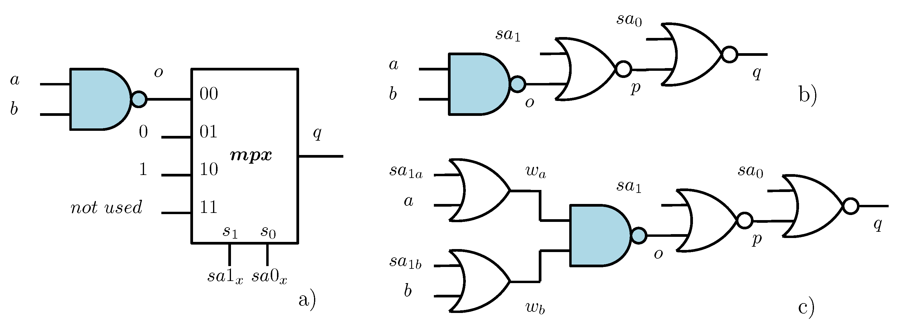
For instance, a multiplexer may be used to select between the module output signal and a faulty value on the basis of selection variables that encode the presence/absence of stuck-at faults affecting such a signal (
Figure 1a). By applying logic simplification and replacing the multiplexer with two gates, an equivalent scheme similar to that used in [
9] can be obtained, as in
Figure 1b.
Such a modified circuit model implicitly describes all possible multiple stuck-ats with no need to explicitly enumerate them as in a simulation. It can be used to build a miter comparing its outputs to those of the fault-free circuit. Some network possibly implementing a cardinality (A) constraint on the fault multiplicity can be added to such a miter. Different fault models can be modeled in a similar way.
In SAT-based approaches, a CNF of this circuit (or of the whole miter) is then built using the Tseitin [
16] or other transformations.
Let us now consider a combinational logic cell with output y and local support x. Under fault-free conditions, let f be the Boolean function implemented by the cell; i.e., . In order to model a fault affecting such a cell, y is replaced in its fan-out by a signal w implementing the function g; i.e., , where denotes the additional signals used to impose either the fault-free value or different faulty behaviors.
For instance, in
Figure 1a,b,
,
,
and
, while the fault-free output function is
In
Figure 1a, a multiplexer is used to inject a stuck-at fault at the gate output; therefore,
o is replaced by
q:
An additional constraint can impose that () holds true, thus avoiding meaninglkess configurations with two faults affecting the same signal.
When using Boolean satisfiability to reason on such a network, a CNF describing all its consistent signal assignments has to be derived.
A more complete model that accounts also for input faults is illustrated in
Figure 1c, where a modified NAND gate accounts for input stuck-at-1 faults as well. It describes all the possible stuck-at fault equivalence classes in a NAND gate. The resulting CNF is
The applications of structural fault injection to fault diagnosis or to the analysis of fault-tolerant properties aim at directly identifying specific faults within the circuit. Consider, for instance, the case of multiple-fault diagnosis: a culprit for a given input/output sequence is a configuration of the set of all the variables of circuit gates that is consistent with the considered input/output sequence.
2.2. Model-Free Approaches
If, in contrast to model-based approaches,
variables are free to vary for the same gate in different circuit copies (similarly to [
7]), we have a fault-model-independent diagnosis, which does not provide a fault dictionary based on stuck-ats (or other modeled faults), but a list of possible fault locations. For instance, in the model of
Figure 1b, it may be possible that some input/output configuration is consistent with
, while others are consistent with
.
In [
11], this problem has been approached by initially considering a structural injection scheme similar to that in
Figure 1a. In particular, a two-way multiplexer is placed at the output
o of a cell, while the other data input is
v and the selection signal is
, thus resulting in the following Equation:
where
q is the new output. Differently from the structural injection scheme in
Figure 1, the input
v is allowed to vary within a diagnosis set of input and output configurations. In fact, in the QBF formulation of the diagnosis problem considered in [
11], such a variable is not bounded, thus allowing for the gate output to have either a faulty or a fault-free value.
Such a description was used in [
11] to derive an injection methodology that allows us to avoid the use of structural modifications and the subsequent derivation of a CNF formula. The fault is implicitly injected within the CNF formula with savings in the number of variables and clauses, while the CNF still represents the possible circuit behaviors in the presence of multiple faults.
In particular, the fault-free CNF of each cell is considered in turn, and a variable is added to all the clauses of such a CNF in order to let the input variables and the output variable be assigned to values that are not consistent with the fault-free function of the cell; then, the clause may still be true by setting as true.
As an example, consider, again, the case of a NAND gate (
) whose CNF describing the consistent assignments to
a,
b and
o:
is rewritten as:
This formula allows for faulty assignments to o, such as, for instance, and , that are justified by setting . It is evident that this new CNF may be satisfied by any faulty behavior, while, in contrast to structural approaches, the number of clauses does not increase with respect to the fault-free case. Note that, in this case, .
2.3. Comparison
In this section, we compare structural and model-free approaches to multiple fault injection by considering a circuit affected by a resistive bridging fault.
In particular, we suppose that a three-input NAND FET cell is affected by an internal resistive bridging fault (
Figure 2a). The detection of this kind of faults depends on circuit and bridging parameters that determine the faulty output voltage of
o. In this example, it is supposed that the fault results in an output error (i.e., a low voltage) when applying input vectors
and 110, while the test 100 does not produce an error because of the increased pull-up conductance. Let us now consider two possible CNFs for the cell: the former corresponds to all the possible input and output stuck-at faults (
Figure 2b), while the latter is a model-free one as in Equation (
8).
In the structural case accounting for input and output stuck-ats, the CNF is
It can be verified that no assignment exists to the variables in that ensures that is satisfied for all values of the inputs and the output of the faulty cell, while for specific values of such variables, there is always a value of satisfying .
In the model-free case, it is
If we set , for any assignment that is consistent with the faulty gate function.
Let us now suppose that Equations (
9) and (
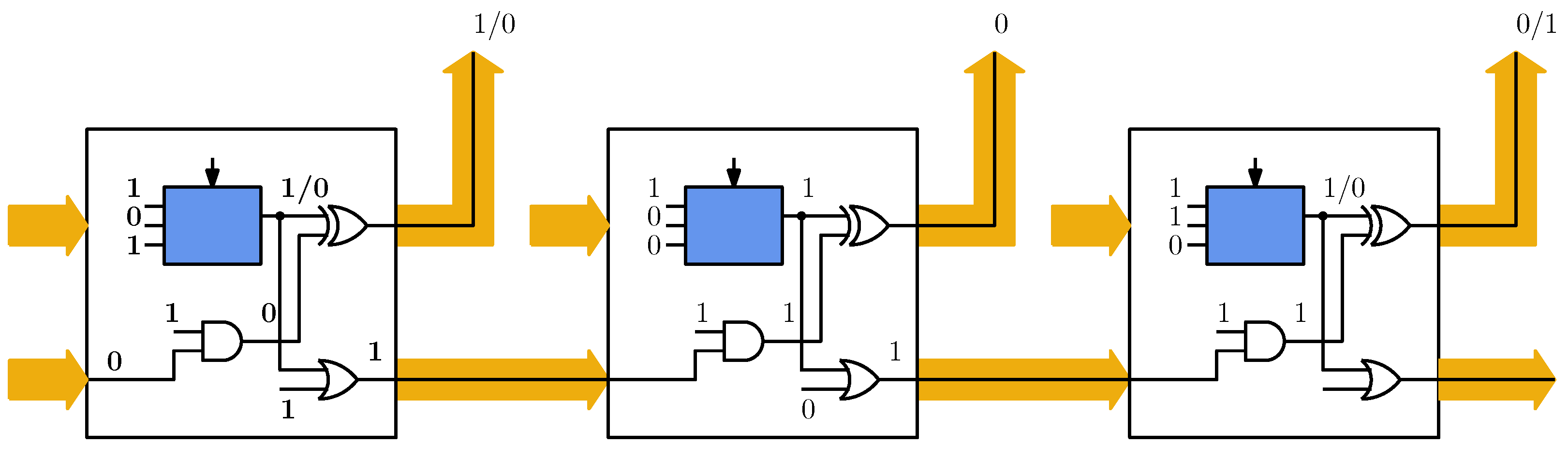
10) are used in a simple fault diagnosis of a synchronous sequential circuit (
Figure 3) where we injected the fault of
Figure 2a in the shaded cell. The figure shows the output values produced by such a faulty cell as they are computed by fault simulation after injection in all time frames. Then, we suppose that, in order to justify such output values, a SAT-based diagnosis tool is applied to the CNF of the circuit in the structural or the model-free approach. In this simple experiment, the only task of SAT is to justify the output values for all time frames, given the input. This can be performed by setting suitable values for the variables in
.
In the stuck-at based case, no single configuration of
may produce the same faulty behavior for all time frames. On the contrary, based on Equation (
9), it is easy to verify that, if different values of such variables are allowed for each time frame, the SAT solver can justify the states of the circuit. Conversely, if the faulty circuit is described by Equation (
10), a single value for
can be used for all frames.
3. Accounting for Realistic Defects
The model-free approach in Equation (
8) implicitly describes any possible kind of faulty behavior of the gate, including not physically realistic ones (for instance, an XOR-like behavior of a faulty NAND gate). This may result in unnecessarily wide fault location sets in the case of fault diagnosis or in some pessimism in reliability analysis.
To approach this problem, while still not using a structural approach encoding all possible faulty behaviors of a cell, we do not use a single additional variable for all the clauses of a cell, but one variable () to be added to clauses featuring the true form literal of the cell output and another one () to clauses featuring the false form literal of the cell output.
In this way, we can describe all faults that results in a monotonic error at the output of a cell: only the on-set but not the off-set of its function, or vice versa, can be affected by the fault. In the case of a NAND gate, this results in
If we do not allow both
and
to be true at the same time, the set of modeled faulty behaviors is restricted to the more realistic cases including internal bridging faults [
13]. This model can be easily generalized to any kind of cell.
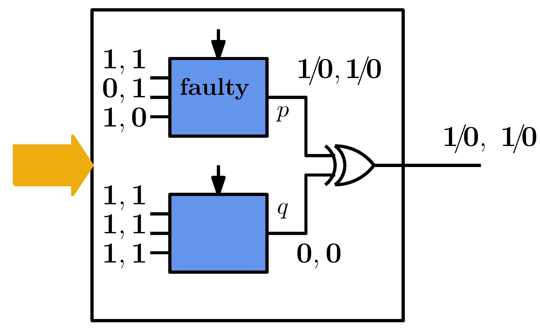
Let us consider again a fault diagnosis experiment over a simple faulty combinational circuit that contains two three-input NAND gates whose outputs are XORed. One of these NANDs is supposed to be affected by the same fault as in
Figure 2a.
Figure 4 shows the cell inputs and the corresponding output values with two input vectors. Let us first suppose that the CNFs of the two cells are described by Equation (
10):
It is easy to verify that a SAT solver (working with the cardinality constraint ) succeeds in justifying the erroneous output value by setting either or , thus meaning that two possible fault locations have to be considered.
Conversely, if we use the proposed approach, the CNFs are
In this case, the SAT solver will provide only as a solution, thus restricting the list of possible culprits.
Other problems that cannot be accounted for by the model in Equation (
8) are related either to faults producing output intermediate voltages such as transistor stuck-ons or internal resistive bridging faults [
13] or to faults affecting interconnections, such as breaks and opens [
12].
In the former case, the gates in the fan-out of the faulty cell may interpret its output faulty intermediate voltage in different ways depending on their actual logic thresholds.
In the latter case, a break or open affecting some position of the layout of an interconnection may cause the gate output value to correctly propagate to a subset only of fan-out gates. This case is shown in
Figure 5 where, with the applied inputs, it is supposed that, because of a break affecting the fan-out interconnects of gate
q, the gates
s and
v receive an incorrect input logic value. The same behavior may occur because of a resistive bridging affecting gate
q and result in its output signal having an intermediate voltage value that is supposed to be interpreted as low by gate
r and as high by gates
s and
v because of statistical variations of the logic threshold of such gates.
In the case of fault diagnosis, a model-free approach cannot justify this condition with a fault cardinality equal to 1, while with a cardinality equal to 2, it would identify s and v as the possible fault locations (or any combination of gates in their transitive fan-out in more complex circuits).
To approach this problem while keeping low values of fault cardinality, we extend fault injection in the CNF by using a different additional variable in each clause of the CNF of a gate, thus providing the following CNF in the case of a NAND gate. The starting point is still Equation (
8), which, in the hypothesis that
a and
b are fan-out-stems, is rewritten as
If one or both inputs are not stem, some simplification can be made, while Equation (
14) can be easily modified to account for unate faults:
By using such an approach, every gate input variable branching out from a fan-out stem is related to an additional variable that we use to describe the possible faults affecting the fan-out branches. Then, we add a stem-related variable () equal to the disjunction of the additional variables related to its fan-out branches. In this way, faults affecting multiple fan-out branches can be reduced to a single fault affecting the fan-out stem.
In order to describe this approach, let us consider the CNF of the gates driven by the fan-out stems
q and
r in the example of
Figure 5:
The CNF of the circuit is completed by the CNFs describing gates
p and
q which use only one
variable because they do not have stems in their fan-in:
The effects of faults affecting the branches of a fan-out stem are then captured by an additional variable holding true if one of the
variables appearing in the clauses containing the stem variable is true. For instance, in the case of
q, we add the variable
as
The same is done for the fan-out stem
r:
Now, a cardinality constraint can be built as the following pseudo-Boolean formula (which can be translated to a CNF):
In this way, the CNF of the whole circuit constrained by the values of primary inputs (PIs) and primary outputs (POs) can be satisfied under the cardinality constraint with a model where the additional variables , and are set true, while other additional variables are set false. Note that if we do not use such additional variables, the CNF can be satisfied only for .
Extension to Combinational Macros
Logic gates do not represent all the possible combinational cells in current and perspective technologies. For instance, this may be the case for the Look-Up Tables (LUT) used in the large majority of Field-Programmable Gate Arrays (FPGAs). This may hold also for perspective technologies featuring small nano-fabrics [
17] or more complex logic gates [
18]. In such cases, our approach cannot be directly applied to a Tseitin transform [
4,
16].
Let us suppose that a Disjunctive Normal Form (DNF) expression is available for both the module output and its complement:
where
and
are product terms. Note that these function representations may often be available during the logic synthesis as a sub-product of two-level logic minimization for single cells. In this case, the CNF for the considered macro can be computed as
(using De Morgan’s laws) where
and
are the literals of the products in the DNF expressions of the module output and of its complement, respectively. This fault-free cell model can be used to inject faults. For instance, if we consider monotonic faults, we can write
Consider a cell implementing the function
; hence,
. The fault-free CNF of such a cell is
The resulting faulty CNF, which can be used to represent all monotonic faults within the considered module, is
For instance, this model accounts for a fault k resulting in a faulty output function equal to , which, in a regular array, may occur because of a missing crosspoint and is not equivalent to any stuck-at fault. For the sake of brevity, the extension of our model to multi-output cells is not discussed in this paper.
4. Results
The proposed approaches can be used to reason regarding several properties of digital ICs in the presence of multiple faults. Without addressing any specific application, we simply compare its efficiency with that of the structural injection schemes reported in
Figure 1b,c. Columns 2–4 of
Table 1 show the characteristics of the considered combinational benchmarks taken from the ISCAS85 [
19] and ITC99 [
20] sets as they are described at the gate level. Moreover, three toy feed-forward integer data neural networks have been added.
Starting from the netlist of each benchmark as it is described in BLIF [
21], we have built the CNF of a miter featuring the conjunction of the fault-free CNF, the CNF describing the faulty circuit (sharing the same variables for PIs), and the CNF of a comparator fed by the POs’ variables of the two copies of the circuit. The CNF of the faulty circuit can be built in different ways depending on the considered fault-injection model:
When considering the model for monotonic faults, we use Equation (
11) to modify the fault-free CNF;
When considering structural models, we used a script to add extra gates to the benchmarks’ fault-free netlist such as in
Figure 1a,b, and then we converted it to a CNF.
The CPU time used to build the miter is negligible with respect to that spent by the SAT solver, and it is not considered.
We initially used the minisat SAT solver [
15]. The experiments were performed on an Intel
® Core™ i7-5500U CPU running at 2.4 GHz with 8 GB of memory under the Linux operating system.
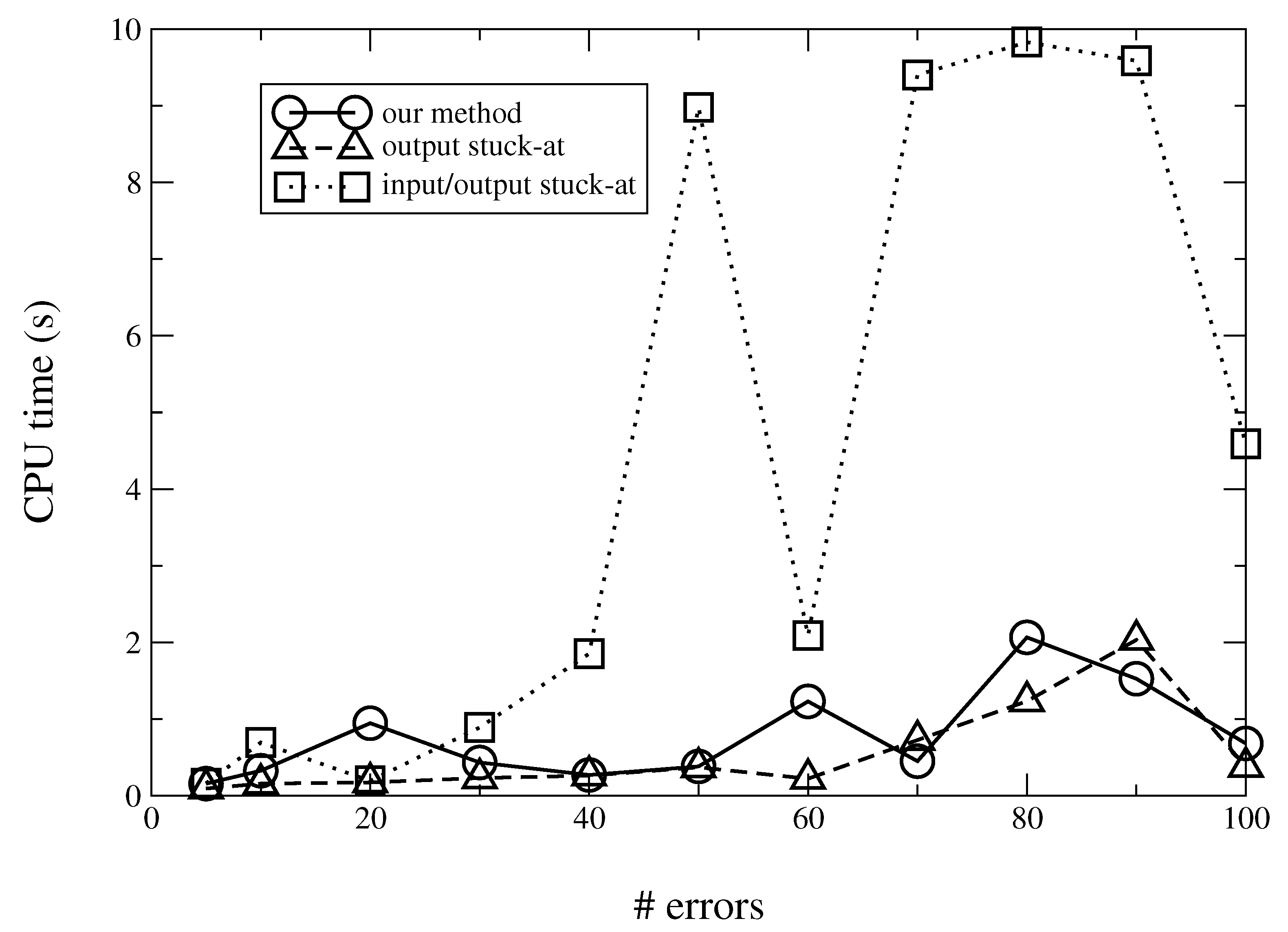
The first experiment aimed at evaluating the computational effort required by a SAT solver in providing a model featuring a number of errors at POs above a given threshold in the presence of an upper bound on the number of internal faults using our approach (Equation (
11)). In some cases, because of such an upper bound, the SAT solver may fail to justify an output error configuration. This problem is common to all the considered techniques and may occur if the number of faults is much lower than the number of output errors.
In particular, the miter’s CNF is augmented by clauses that allow us to count the number of errors, E, and the number of variables at 1, A (which we consider as the fault cardinality). This allows us to set constraints on the minimum number of errors, , and on the maximum number of faulty cells, .
The larger and the smaller are, the larger the computational effort is expected to be, because we prevent the SAT solver from producing trivial solutions featuring a large number of faulty cells in the vicinity of POs. Such an experiment is only used to characterize the computational costs of the different modeling techniques in a way that is independent of the specific kind of application.
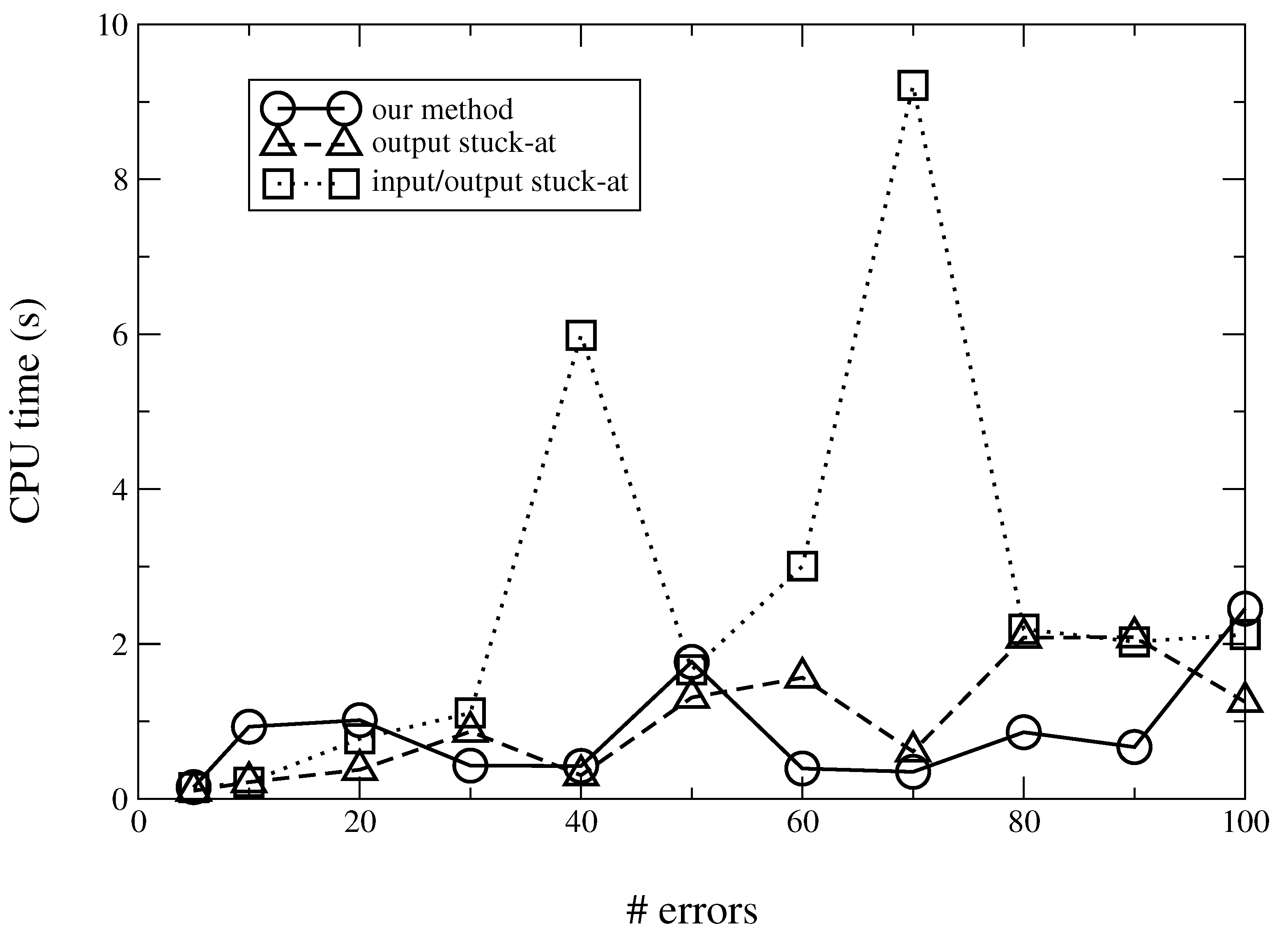
This is illustrated in
Figure 6, which, for the benchmark b14, reports the CPU time as a function of
, with
. The figure shows the results achieved by three considered methods. As expected, the CPU time increases with the minimum number of errors to be justified, even though the curves are non-monotonic because issues such as the circuit topology affect the execution of the SAT solver with different targets on errors. Moreover, the relevant computational cost of input/output fault injection can be noted.
The CPU time and the number of clauses (
c) are shown in
Table 1 for all benchmarks when considering (i) fault injection at gate output, (ii) stuck-at injection at gate inputs and output and (iii) our method. These data have been computed using
and
.
As can be seen, the model featuring output stuck-ats and the proposed approach perform in a similar way (489 s on average compared to 462 s): such large values, however, are not suitable for several kinds of applications.
4.1. Cardinality of Faults
The analysis of the above-mentioned example shows that the cardinality constraint on the number A of faulty cells poses a relevant computational problem because of the size of the adder networks used to count variables: in fault diagnosis or when verifying some fault-tolerant property of circuits, such cardinality constraints may be required. This worst-case scenario is common to all the considered techniques.
Any constraint on
A can be expressed as a Pseudo Boolean (PB) one and can be translated to Boolean constraints by using a ones counter, which is a complex arithmetic network featuring several adder circuits; as an alternative, it can be obtained by using the PB-to-Boolean conversion embedded in a PB SAT solver such as minisat+ [
14], which can use also combinational sorters which, however, do not provide benefits. The additional constraints due to the presence of such a network lead to relevant overheads in the time spent by the SAT solver.
To mitigate this problem, we used a simple approach based on a symbolic ordinate-based decoding of faults that, for , becomes an -decoding, used to illustrate this approach. We suppose that a faulty cell can be selected by the outputs of two decoders (x and y) and, as shown below, we perform this operation with no need to explicitly model the decoders. This operation works when considering single faults; in the case of multiple faults, we need to add pairs of decoders up to fill the maximum fault multiplicity. In this way, if n is the number of faulty cells, we reduce the size of the cardinality constraint from to approximately .
Such a strategy can be applied to any of the considered methods and is here instantiated only in our case. Consider the model describing monotonic errors, featuring two variables (
and
) per cell and a maximum fault multiplicity for the whole circuit equal to 2. Then, for the
i-th cell (
), which is supposed to be mapped on ordinates
(for which approximately holds
),
where
is the output of the
x-decoder connected to such a cell and
is the output of the
y-decoder for the same cell.
and
play the same role for a second decoder. The number of such signals is proportional to
. Note that the pair of variables
,
is different for each cell of the circuit.
Now the (PB) cardinality constraint can be moved to the outputs of the decoder: the arithmetic sum of the outputs of each of them (that is ) must be no larger than one.
If the solver needs to inject faults in two cells, two different pairs of variables will have their conjunction at 1; otherwise, if the fault has to be injected in one cell only, then either only one pair of variables has the conjunction at 1 or the two pairs corresponding to the same cell will be at 1.
Of course, by adding a suitable number of decoders, this technique can be generalized to any maximum cardinality in the number of faulty cells.
The results achieved by using this technique with our method are reported in the last column of
Table 1, showing a remarkable speed-up (27 times) that results in an average CPU time equal to 17 s.
4.2. Application to Complex Modules
The approach described in
Section 3 has been applied to an FPGA implementation of the benchmark b14 obtained by mapping such a circuit with abc [
22] on four and five-input LUTs. In this regards,
Figure 7 and
Figure 8 show the CPU time for
and different values of
for the four-input LUT and the five-input LUT, respectively. Each figure shows the CPU time for the injection of faults at cell output, cell inputs and output and our method.
As can be seen, the CPU time, computed without using
-decoding, is lower than in the gate-level case, because of the smaller total number of
variables.
Table 2 summarizes the results achieved for the set of considered benchmarks mapped on four-input and five-input LUTs by considering the same conditions (
,
) used to obtain the data in
Table 1.
The computational costs are smaller than in the gate-level case for all benchmarks.
4.3. Faults in Fan-Out Stems
As an application of the proposed method for faults in fan-out stems, we have considered a simple experiment partially emulating the operations of fault diagnosis. The target is to analyze the feasibility of the metho d outlined in
Section 3 for faults resulting in breaks or intermediate voltages at fan-out stems.
To this purpose, we have initially used the c6288 benchmark that is a parallel multiplier. In our experiment, we have considered a set of possible diagnosis instances, each of which are constrained to present one of the possible (496) double errors at POs and a random input configuration.
For each instance, three different CNFs have been generated. The first one (to be referred to as case 1) uses the model in Equation (
8) and a fault cardinality equal to 1. The second one uses the same model, but a cardinality equal to two (case 2). The third one, instead, uses the proposed model (Equation (
14)) accounting for fan-out stems with a cardinality equal to 1 (case 3).
In case 1, only one cell may be faulty and the SAT solver is able to justify only 14 samples out of 496. In fact, even if several cells exist in the intersection of the transitive fan-ins of the two erroneous POs, an error in such cells may propagate also to other POs, thus resulting in an unsatisfiable instance. Of course, when considering a cardinality equal to two (case 2), we had 480 out of 496 satisfiable instances. The same result is obtained with the model considering fan-out stems (case 3), where we may have only one faulty stem.
The main difference between cases 2 and 3 is in the average number of possible solutions per instance, which are 354 and 129, respectively. From the point of view of fault diagnosis, this shows that the proposed technique (3) is capable of identifying faults possibly originated by a single defect. Conversely, by injecting faults at the cell level (2), additional solutions () are produced that correspond to multiple defects. From the point of view of the average CPU time spent by the solver, it is 0.47 s in case 1, while in cases 2 and 3, it is almost the same (0.81 s and 0.89 s, respectively).
This analysis has been performed also for the other benchmarks considered in
Table 1. In some cases, because of the large number of outputs and, consequently, of possible double output errors, only a sample of 1000 of this kind of errors has been considered. The achieved results are summarized in
Table 3, reporting for each method the percentage of satisfiable instances and the CPU time (computed using minisat+ with only combinational sorters as cardinality encoders). As can be seen, the CPU time in cases 2 and 3 is similar, thus showing that the additional
variables do not give rise to relevant computational overheads. In addition, the table reports the number of solutions per sample provided by case 2 and by our method. These last results show that, when considering defects affecting fan-out stems, we always achieve a reduction in the number of cases to be considered by fault diagnosis.
4.4. Application to New Test and Verification Paradigms
The verification of fault-tolerant properties may require the determination of the minimal fault cardinality producing an output error. Moreover, the test generation for approximate computing may require unconventional approaches that generate tests maximizing some numerical difference between the faulty and the fault-free outputs. These are optimization problems that can be solved by PB SAT solvers/optimizers [
14].
In the case of fault-tolerant circuits, we do not target specific applications, but we want to analyze the computational costs required to characterize worst-case scenarios from the point of view of errors when using the model described in Equation (
11) for multiple faults resulting in monotonic errors. Therefore, we considered two general problems requiring the computation of (1) the maximum number of errors related to a given fault multiplicity and (2) the minimum number of faults producing a number of errors above a given threshold.
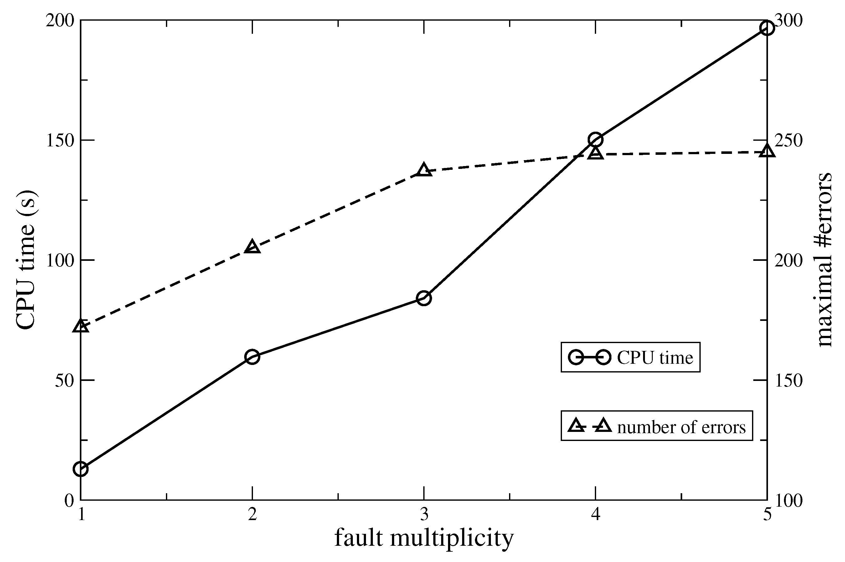
In case 1, at first, we considered the gate-level implementation of the benchmark b14 and we formulated the following PB optimization problem: maximize the number of output errors (
E) for a given fault multiplicity
. Note that, in doing so, we did not exploit structural information.
Figure 9 shows the results achieved by the PB solver/optimizer minisat+ using sorters to encode cardinality constraints (here, sorters work better than the adders used in the previous section).
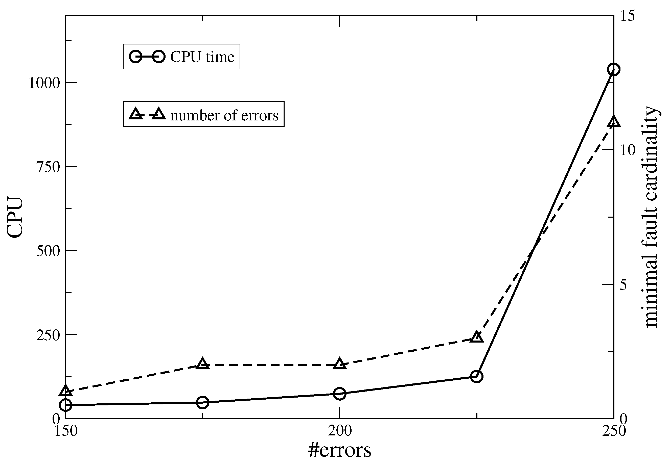
The data achieved for the inverse problem (case 2) are shown in
Figure 10, which reports the CPU time used to minimize the number of faulty cells in order to achieve a target number of errors. As can be seen, the CPU time scales in the worst way with respect to case 1 because the number of faulty cells is much larger than the number of possible errors.
Now, we use the simple feed-forward neural network nn0 to instantiate the cases, requiring us to quantify the error due to multiple faults from a numerical point of view. Such a network features three output words corresponding to three complement-two encoded integers. Let
be such output values in the fault-free case, while let
be the corresponding values in the presence of multiple faults. In our experiment, we generated a CNF implicitly modeling a miter that describes (1) the fault-free circuit, (2) the faulty circuit (using our method) and (3) a comparison logic which, for each output word, checks for the accuracy of the result by comparing the absolute value of the difference of the fault-free and faulty words to a constant (
). Each comparator produces an error signal
:
The CNF describing such a miter has been used to formulate the following PB problems: (1) determine the minimal number of faulty cells that result in for and (2) solve the same problem as in (1) but with constraints on the weights of neurons that have been randomly assigned. In case 1, the CPU time spent by the PB SAT solver/optimizer to provide the minimum () is equal to 255.40 s. In case 2, the CPU time has been computed for 100 different sets of random weight values, resulting in a mean value equal to 220.87 s and a standard deviation equal to 68.32 s. In this latter case, the minimal value of A ranges in the interval from 1 to 3 where the values larger than 1 are obtained only if several weights are at logic 0.
The results achieved using the PB optimizer show that, for modules of small size, testing and verification problems requiring optimization can also be approached.


