Article

SAPF Parameter Optimization with the Application of Taguchi SNR Method

by
Jitendra Kumar Sao
1,
Ramasamy Thaiyal Naayagi
2,*,
Gayadhar Panda
3,
Ram Dayal Patidar
1 and
Sushree Diptimayee Swain
1
1
Department of Electrical Engineering, O.P. Jindal University, Raigarh 496001, India
2
School of Electrical and Electronic Engineering, Newcastle University in Singapore, Singapore 567739, Singapore
3
Department of Electrical Engineering, NIT Meghalaya, Shillong 793001, India
*
Author to whom correspondence should be addressed.
Electronics 2022, 11(3), 348; https://doi.org/10.3390/electronics11030348
Submission received: 31 December 2021 / Revised: 12 January 2022 / Accepted: 19 January 2022 / Published: 24 January 2022
(This article belongs to the Special Issue Advances in Low Power and High Power Electronics)

Abstract

:
Non-linear devices draw non-sinusoidal currents from the source; hence, they cause harmonic distortions in power systems. The shunt active power filter (SAPF) is a well-known method for alleviating current harmonics, compensating the reactive power and improving the power factor; however, the effective design of an SAPF is quite challenging and a thrust area of research. The current controlling technique, switching pulse generation technique and parameter selection are cumbersome tasks in SAPF design. SAPF performance depends on the proper selection of many parameters, such as filter interfacing impedance, DC-link capacitor and PI-controller gains. The effect of these parameters on the performance of SAPF has been studied and optimum values have been obtained by using the Taguchi method. This paper also indicates the benefits of using the Taguchi method compared with existing genetic algorithm (GA) for optimizing the parameters of the SAPF. An instantaneous reactive power theory (IRPT)-based SAPF has been modeled and simulated in MATLAB/Simulink. The SAPF’s parameters have been optimized by using the both proposed Taguchi SNR and the existing GA method. With optimized values of parameters results have been obtained, analyzed and the superiority of the proposed Taguchi method over the existing GA method is discussed. The simulation results were also validated with experimental results.

1. Introduction

Harmonic contamination is a major issue in power systems, because of the tremendous usage of power electronic equipment and various non-linear loads in recent years. Harmonic interference adversely affects the power quality under many aspects, such as, given that most of power electronic equipment is non-linear in nature, when used as a load, it draws a non-sinusoidal current from ac sources, hence generating undesirable current harmonics in the supply side, degrading the power quality [1]. Low power quality may damage the sensitive equipment and cause a huge loss in the industry. Many methods of harmonic mitigation have been studied and suggested by researchers. The passive filter is one of the simplest methods of harmonic compensation. Passive filters are designed using passive storage elements, mainly, inductor and capacitor. Passive filters are simple, reliable and cost effective, but they have major disadvantages, such as resonance problems and static compensation. Because of these drawbacks, active power filters (APFs) have become very popular as power conditioning devices for harmonic and reactive power compensation [2].
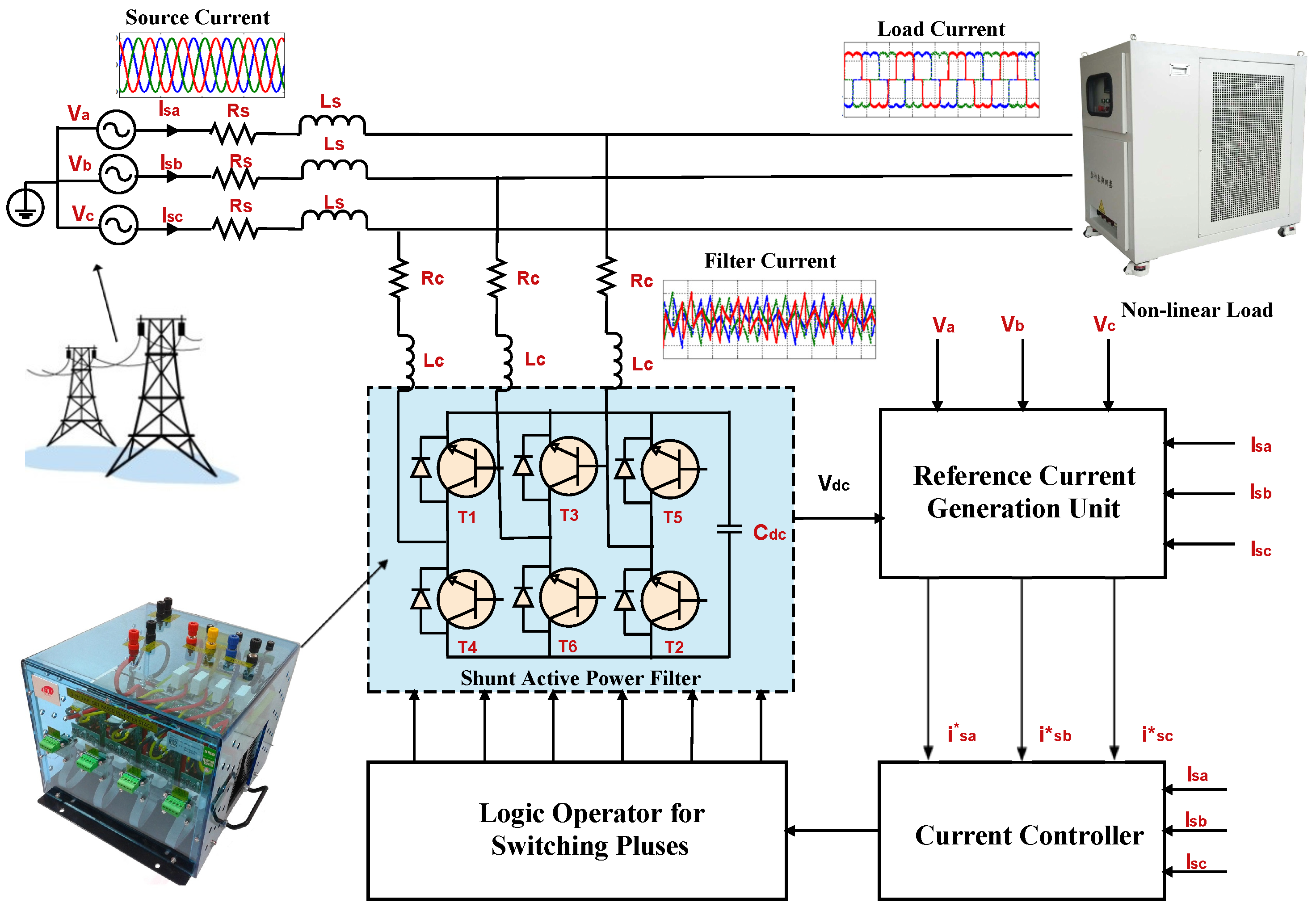
For current compensation, an active power filter (APF) should be connected in parallel with the source and load, so that the APF can inject filter current, which compensates the unwanted generated harmonics due to a non-linear load. The generated filter current should be just equal in magnitude and opposite in phase to the generated unwanted harmonic current for proper compensation. An active power filter is a power conditioning device which provides reactive power compensation and a load balancing solution in conjunction with harmonic compensation. A detailed review of active power filters with different configurations, control strategies, component selection and their selection criteria for specific applications is presented by Bhim Singh et al. [
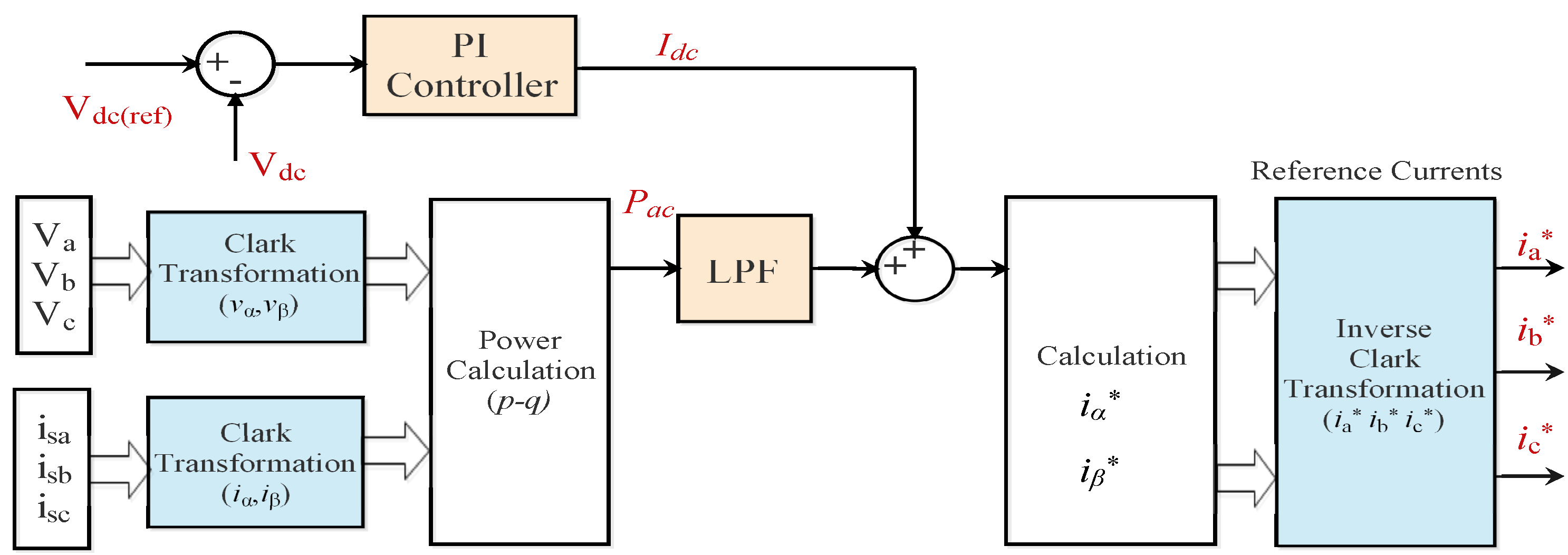
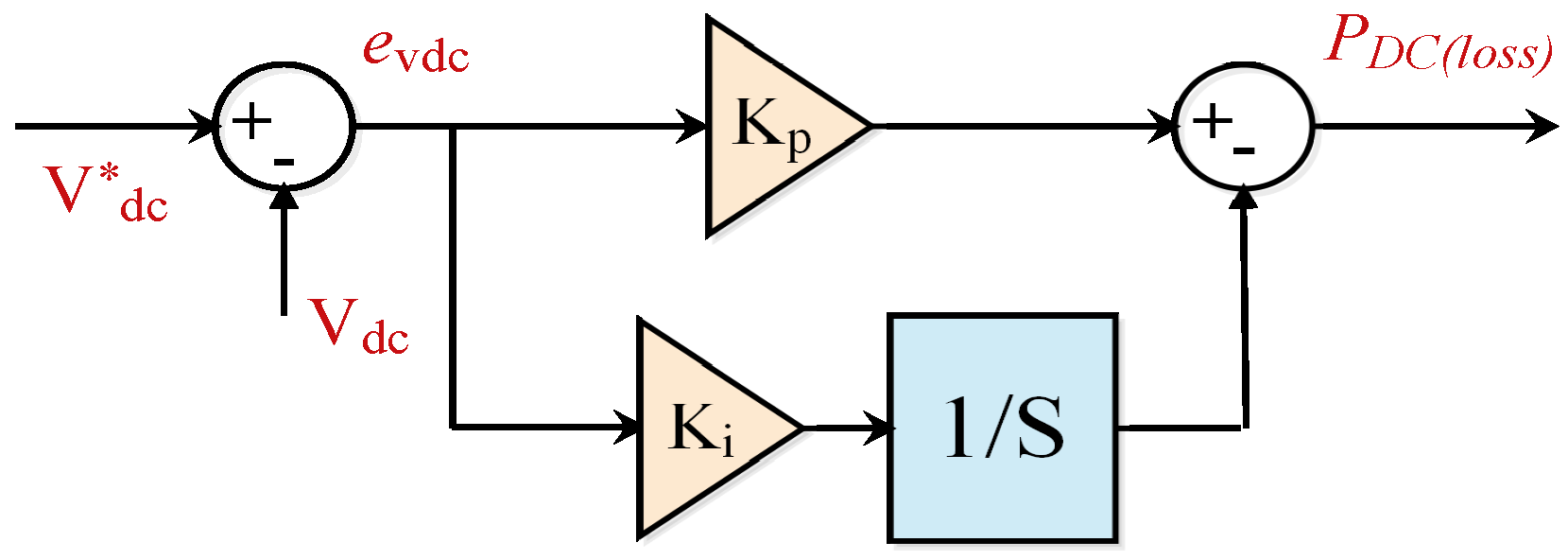
3]. There are mainly four kinds of controlling evolved in the design of SAPFs, i.e., (1) controlling of current reference generation or harmonic extraction; (2) controlling of DC-link capacitor voltage ( V d c ); (3) controlling of switching pluses; (4) controlling of synchronization [4]. The performance of SAPFs depends on the effectiveness of these controlling algorithms as well as proper selection of parameters.
There are many design parameters that affect the performance of SAPFs, such as gain of PI controller gains ( K p and K i ), DC-link capacitor ( C d c ) and interfacing impedance ( R c and L c ) of SAPFs. To extract the maximum performance for SAPFs, these parameters must be optimized. Some of these parameters have been optimized in earlier literature studies, such as Bruno A. Angelico’s use of a bode diagram for proportional-integral tuning for single-phase active power filter [5]. The artificial bee colony optimization method has been implemented for optimal load compensation by SAPFs [6]. Soft computing techniques, such as artificial neural network (ANN) and fuzzy logic controllers, have been used for designing SAPFs [7,8]. Hany M. Hasanien used the Taguchi method for optimizing PI controllers in cascaded control systems [9]. The genetic algorithm (GA) was used for the tuning of the controller by Pericle Zanchetta [10]. The design parameters of SAPFs have also been optimized by using the genetic algorithm approach by Hien [11]. In spite of optimizing the parameters, none of the above-mentioned optimization methods provides information about the sensitivity of the parameters on the performance of SAPF compensation. The Taguchi method not only optimizes the parameters but also gives information about the sensitivity of the parameters on the performance of SAPF compensation. In Taguchi methods based on the difference in SNRs, a rank is allotted to each parameter which signifies the sensitivity of the parameters. The parameter variation in a more sensitive parameter affects results the most in the performance of SAPFs. Parameter’s sensitivity prediction is not possible in the genetic algorithm.
This paper proposes a new Taguchi SNR-based optimization method for the optimum selection of SAPF parameters [9]. This manuscript is organized as follows: The configuration and proposed control structure used for SAPF designing are described in Section 2; the optimization of SAPF parameters using the Taguchi method is given in Section 3. Section 4 describes the optimization of SAPF parameters by using the existing genetic algorithm method and simulation results and their analysis for both the existing and proposed methods. In Section 5, the experimental results and their analysis for both the existing and proposed methods are given. Finally, some conclusions are discussed in Section 6.

2. Shunt Active Power Filter

2.1. Filter Configuration

Harmonics generated due to a non-linear load can be compensated by passive filters or active filters. A passive filter is made up of passive components, such as resistor, inductor and capacitor; hence, an active filter is made up of active components. A passive filter is simple in design, but, due to the presence of the inductor, it is bulky in nature. In addition, passive filters have major disadvantages, such as resonance problems and fixed compensation; therefore, for practical application, active filters are more suitable for harmonic compensation, as they have better flexibility and performance than passive filters. To suppress the current harmonics in the source current due to a non-linear load, an active filter, known as shunt active power filter (SAPF), is connected in parallel to the load. For our experimentation, a three-phase rectifier was considered as the harmonic-generating load. This load was connected with an AC supply with source impedance ( R s and L s ). This three-phase uncontrolled rectifier was a non-linear load and drew non-sinusoidal current from the AC supply; hence, it caused harmonics in the source current. To suppress these undesirable harmonics, an active power filter was connected in shunted form between the harmonic-generating load and the AC main supply. This SAPF supplied the compensating current at the point of common coupling (PCC). The SAPF configuration is given in Figure 1.
The SAPF mainly consists of four main segments; the first is necessary to measure the required voltage or current signals, the second is required to generate the reference current, the third is required to regulate DC-link capacitor voltage ( V d c ) and the fourth is required to generate the switching pulses with the IGBT switches of the voltage source inverter (VSI) of the SAPF. For proper compensation, the reference current should be the same in magnitude but out of phase in respect to the unwanted harmonic current. The voltage source inverter is connected at the point of common coupling with the filter interface impedance. To operate the VSI, a DC-link capacitor ( C d c ), which stores energy, is connected to it. This VSI is controlled by switching pulses generated from a current controlling section. Finally, the control unit compares the reference currents with the sensed actual feedback currents measured at the output of the inverter and provides proper switching pulses by the logic operator unit.
The SAPF’s compensation performance can be measured by evaluating the total harmonic distortion (THD) of the source current with and without the SAPF. The THD of the source current is defined as the ratio of the root mean square (RMS) value of the sum of all harmonic components and the RMS value of the fundamental component of the source current, as given by Equation (1).
T H D = 100 × h = 2 I h I 1 2
where h is the order of the harmonics, I h is the hth harmonic source current and I 1 is the fundamental component of the source current; THD is given in percentage (%).

2.2. Reference Current Estimation

The most popular and simple method to estimate reference currents is the instantaneous reactive power theory (IRPT), also known as the p-q theory, which was proposed by Japanese electrical engineer and Professor Hirofumi Akagi in 1996. The block diagram of the proposed reference current generation p-q algorithm is given in Figure 2.

2.3. P-I Controller for DC-Link Voltage Regulator

The transfer function of the conventional proportional-integral (PI) controller is given in Equation (2).
H ( s ) = K p + K i S
where K p and K i are the proportional and integral constants of the PI controller.
The PI controller is shown in Figure 3. The PI controller regulates the DC-link capacitor voltage ( V d c ) and estimates the peak value of the reference currents. The PI controller is also responsible for the dynamic response and settling time of DC-link capacitor voltage ( V d c ) and dc-power losses ( p D C ( l o s s ) ). The PI controller provides the peak value of the estimated source or reference current.
In order to calculate the error, the measured DC-link capacitor voltage is compared with the desired value. The output of the DC-link capacitor voltage regulator is considered as P D C ( l o s s ) and is given by Equation (3).
P D C ( l o s s ) = K p + K i S × e v d c
where e v d c is the error DC-link voltage.

3. Taguchi Method for Optimization of SAPF Parameters

As other methods of optimization, such as genetic algorithm and particle swarm optimization, are not capable of describing the sensitivity of the parameters on the performance of an SAPF, the Taguchi method of optimization was used for this experimentation. The Taguchi Method is a statistical approach of parameter optimization introduced by Japanese engineer and statistician Genichi Taguchi in 1995 [12]. The Taguchi method is not only capable of optimizing many parameters with lesser experimentation but also provides information about the effect of parameter variation on the performance of an SAPF based on the sensitivity of the parameters. Earlier, the Taguchi method has been mainly used to optimize the process parameters in manufacturing to improve the quality of the goods manufactured. Later, researchers have expanded its application in other fields of engineering. R.S. Rao et al. have discussed Taguchi method applications in biotechnology [13]. R. Davis and P. John have presented Taguchi method applications in industrial chemical processes [14]. A. Sorgdrager et al. have explained the use of the Taguchi method in electrical engineering [15].
In the Taguchi method, the first parameters that need to be optimized are selected; then, a set of experiments is conducted as per orthogonal array (OA). After conducting the experimental run, the results are analyzed using the signal-to-noise ratio (SNR) to obtain the optimum values of the parameters and, finally, a verification run is conducted by taking the optimum values of the parameters obtained from the Taguchi method. Taguchi’s method for parameters requires the following steps [16]:
  • Identify the function to be optimized.
  • Identify the controlling parameters and their levels.
  • Select a suitable orthogonal array (OA).
  • Perform a matrix experiment and obtain results.
  • Examine the results by SNR for optimization.
  • Perform a verification experiment.

3.1. Identifying the Function to Be Optimized

The main idea of designing a shunt active power filter is the mitigation of the harmonics generated by a non-linear load. Harmonics are measured by total harmonic distortion (THD). So, the main purpose of SAPF design is to minimize the THD. With the implementation of an SAPF, the THD should be less than 5%, as per IEEE Std.519. The smaller the THD, the better the SAPF; hence, we considered that a smaller SNR ratio was better for analyzing the results.

3.2. Identifying the Control Factors and Their Levels

The proper selection of the parameters is necessary for successful implementation of an SAPF. The selection of the parameters affects the performance of the SAPF. There are many parameters, such as the gain of the PI controller ( K p and K i ), coupling register ( R c ) and inductor ( L c ), and the DC-link capacitor ( C d c ) affects the performance of the parameters; hence, the proper selection of these parameters is necessary to obtain optimum performance of the SAPF. For our experimentation, we selected five parameters—coupling resistor ( R c ), coupling inductor ( L c ), PI controller gain parameters ( K p and K i ) and DC-link capacitor ( C d c ). Due to the lack of accuracy values of these parameters, we manually selected four different levels of these parameters. The Taguchi method reduces effort and time to find an optimum set of these levels. The purpose of implementing this method is to efficiently determine the optimum set of these parameters for achieving the least THD. The parameters and their level are shown in Table 1.

3.3. Selecting a Suitable Orthogonal Array (OA)

The selection of an orthogonal array (OA) depends on number of factors and number of levels selected for experimentation. Taguchi uses the following convention for naming the orthogonal arrays L N ( S K ) : N = total number of trial during experimentation, S = number of levels for each factor and K = number of parameters or factors. Taguchi’s design can have many factors with several levels. This method requires a lower number of experiments than traditional full factorial designs. For our experimentation, we considered five factors with four levels. The full factorial design method would have required 4 5 = 1024 experiments, while the Taguchi method required only 16 experiments to obtain the optimum set of parameters. An orthogonal array (OA) should be selected so as to obtain proper optimum results with as few runs as possible. For our experimentation with five factors with four levels, a standard L16 orthogonal array meets the above criteria. The L16 orthogonal array was selected for the experimental matrix.

3.4. Performing Matrix Experiments and Obtaining Results

After selecting a suitable orthogonal array (OA), the experimental matrix was constructed according to the selected orthogonal array (OA). As per the experimental matrix, the experiments were performed and the results were collected. These results were used for calculating the signal-to-noise ratio. For our experimentation, we selected an L16 orthogonal array; hence, we had to perform a total of 16 experiments using this method, instead of 1024 experiment using a full factorial design method. The experimental matrix and results (THD) are noted in Table 2.
Our objective function THD was used for calculating the SNR. The objective function (THD) is a “smaller-the-better”-type of control function i.e., the smaller the THD, the better the performance of the SAPF. The signal-to-noise ratio for the “smaller-the-better”-type objective function could be calculated from Equation (4).
η = 10 log 10 1 n i = 1 n y i 2
where η is the signal-to-noise ratio in dB and y i is the output which is needed to be optimized; in this case, y i is the THD.
The SNRs for all 16 experiments were calculated and tabulated in Table 3.
The average SNR for the individual control factors and for each level is tabulated in Table 4. Table 4 also contains the sum of the differences in SNRs for each level of individual control factors. Based on the sum of the difference, the control factors were ranked. The larger the sum of the difference, the more sensitive the parameter. As we can see, L c had a grater sum of difference; hence, it ranked first, i.e., L c was the most sensitive parameter and any variation in the L c level affected the most the SAPF’s performance; hence, the THD changed the most with any variation in L c . Similarly, R c had the least sum of difference; hence, it ranked fifth, showing that the variation in the R c level affected the least the SAPF’s performance and THD. The rank identification of parameters is not possible in soft computing techniques such as the genetic algorithm.
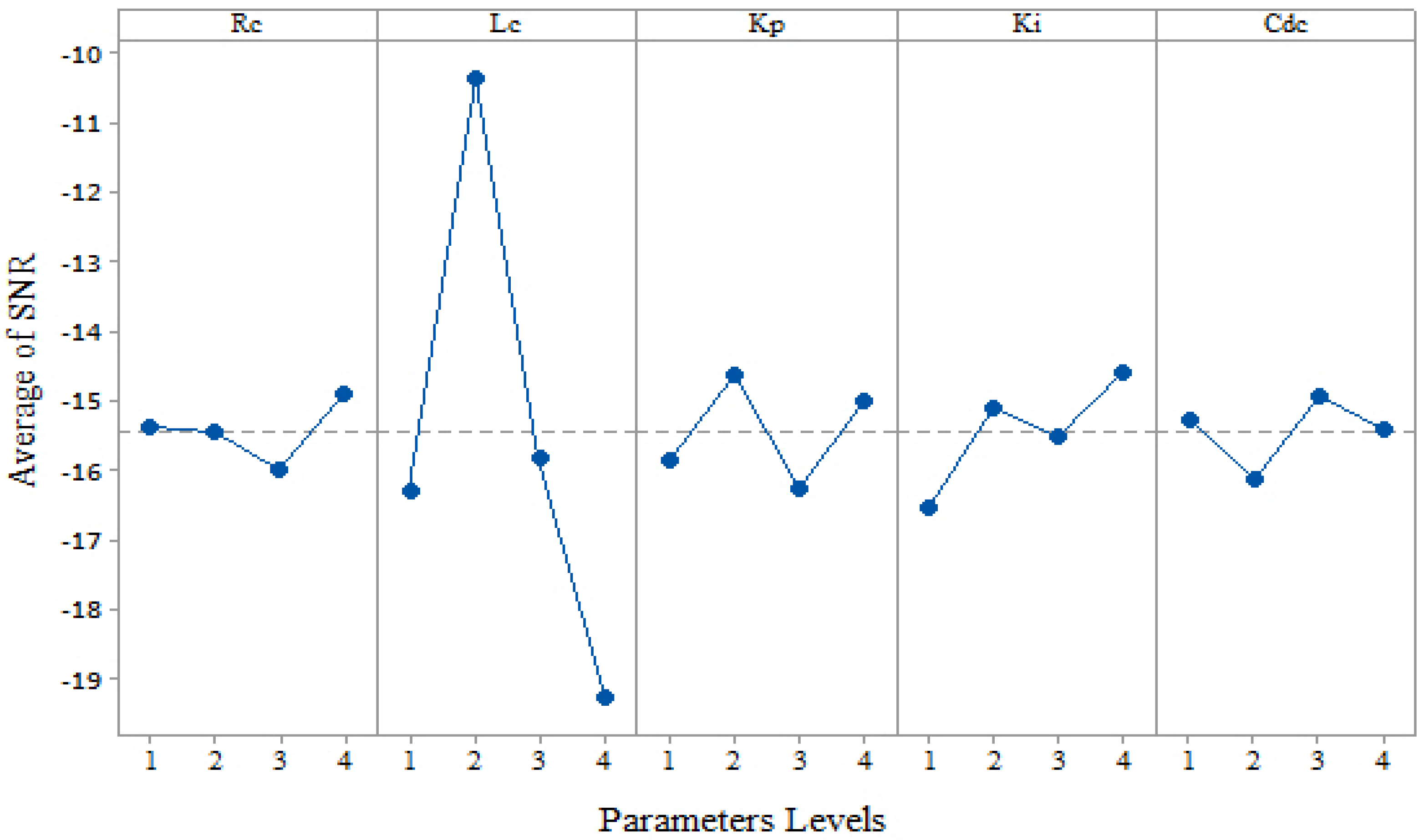
The factor level having the highest SNR is the most optimized level of that factor. From Table 4, a linear graph was drawn, shown in Figure 4. In Figure 4, it is clear that the optimum levels of the parameters R c , L c , K p , K i and C d c were level 4, 2, 2, 4 and 3, respectively.
Table 5 contains the optimum level of the parameters with their optimum values for obtaining the least THD. Using this Taguchi method, we obtained the optimum levels by only conducting 16 experiments instead of conducting 1024 experiments, as we would have had to do adopting a full factorial design.

3.5. Performing A Verification Experiment

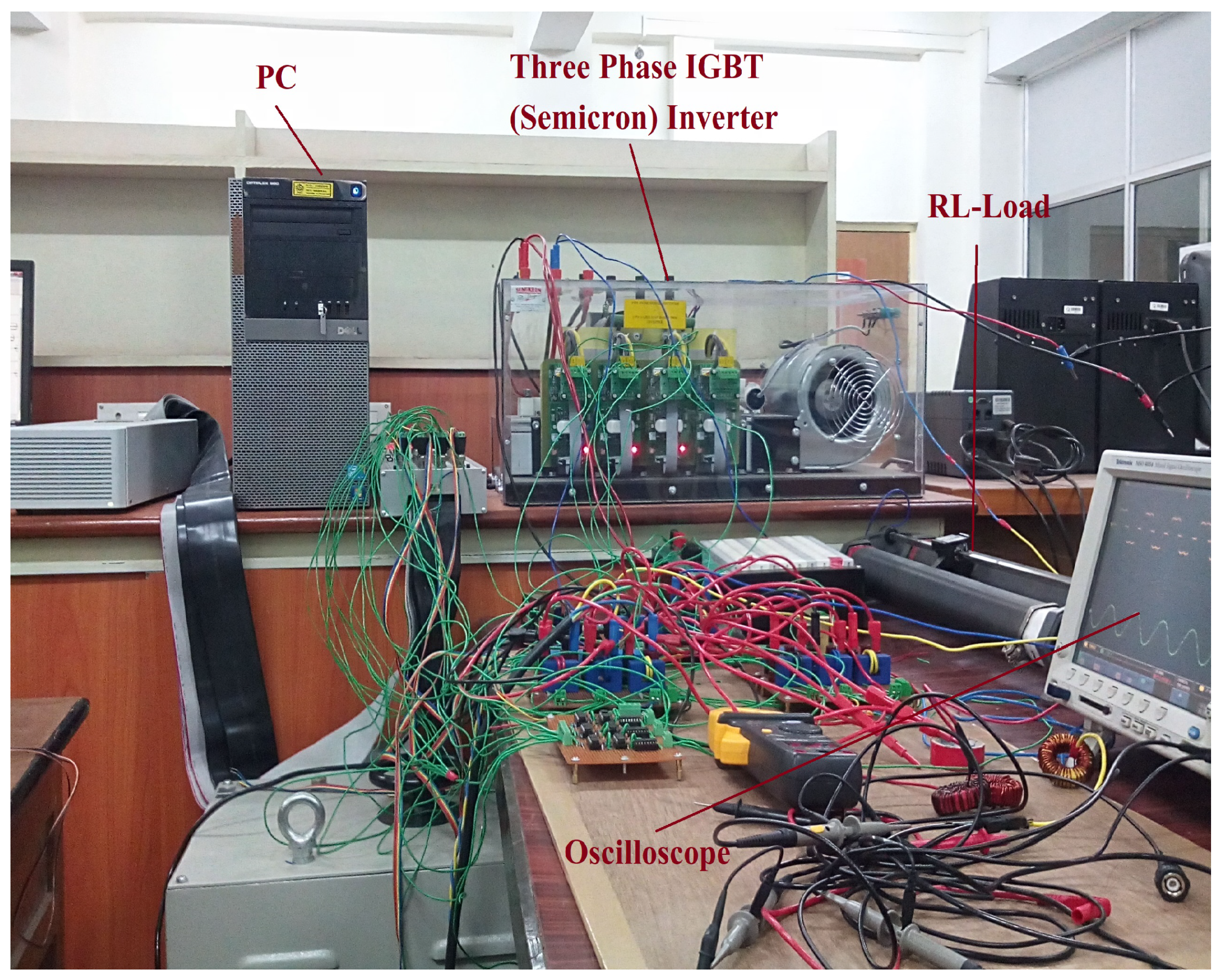
After obtaining the optimum levels of the parameters, a verification experiment was performed by taking the optimum values of these parameters (i.e., R c = 100 m Ω , L c = 1 mH, K p = 0.05, K i = 10 and C d c = 30 μ F) with a three-phase bridge rectifier, with R-L taken as the load. After performing the experiment, the THD was reduced to 2.88%, which is the lowest among all the possible combinations of the above parameters’ values.

4. SAPF Parameter Optimization by Genetic Algorithm

The genetic algorithm (GA) is an intelligent searching method inspired by the genetic laws of reproduction and natural evolution. The GA was proposed by J.H. Holland in 1992. The GA includes initialization of population, defining fitness function, selection, crossover, mutation and checking termination condition. The set of individual parameters which is a solution of a problem is called population. Initially, a population is randomly initialized, but basic parameters of the GA, such as chromosome length and population size, must be specified. A fitness function is used to determine the fitness of an individual population. Better fitness means a better individual, with better chances of survival. The selection process is used to select the fittest individuals for reproduction and for passing their genes to the next generation. Crossover is the process of interchanging genetic properties between two chromosomes to obtain the next generation. Mutation is the process of changing the values of genes of chromosomes after the crossover process. After the selection, crossover and mutation operations, a new population is generated that is better adapted than the previous generation. This algorithm is completed when the fitness function achieves maximum value or the stopping criteria are reached.
For comparing the optimization result with the Taguchi method, we took the same initial condition used in the Taguchi method. The fitness function was the THD as given in Equation (5) and the same range of parameters was considered. The lower and upper boundaries of R c , L c , K p , K i and C d c were considered as [0.1–100] m Ω , [0.5–2] mH, [0.01–0.5], [0.01–10] and [10–40] μ 
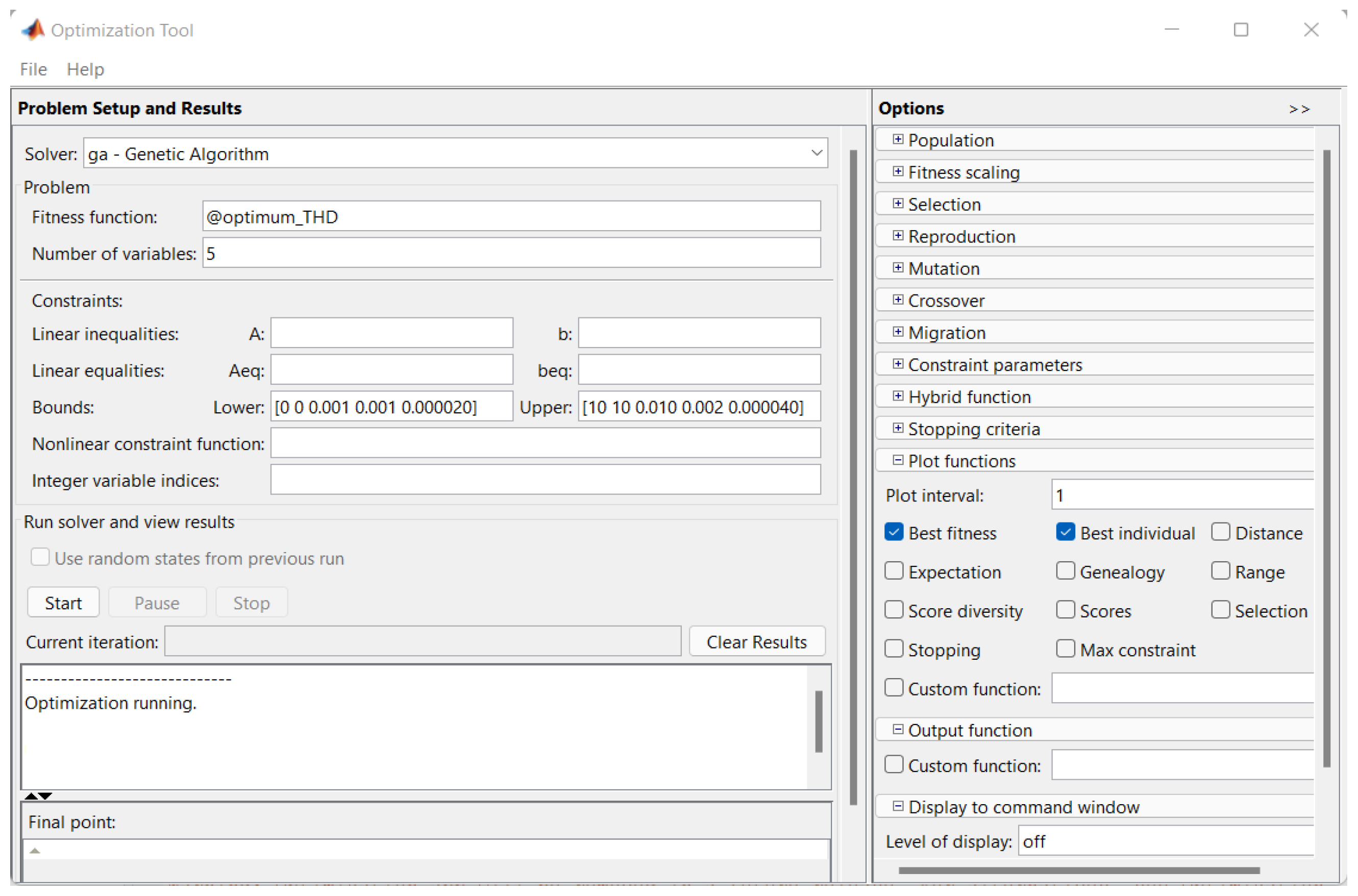
F, respectively. The MATLAB optimization toolbox was used for optimizing the parameters using the GA as shown in Figure 5. The initial population was set to 4 and the maximum number of generations was set to 16 for the experimentation. The stochastic uniform selection criterion was chosen. Scatter crossover and uniform mutation were used for optimization.
T H D = f ( R c , L c , K p , K i , C d c )
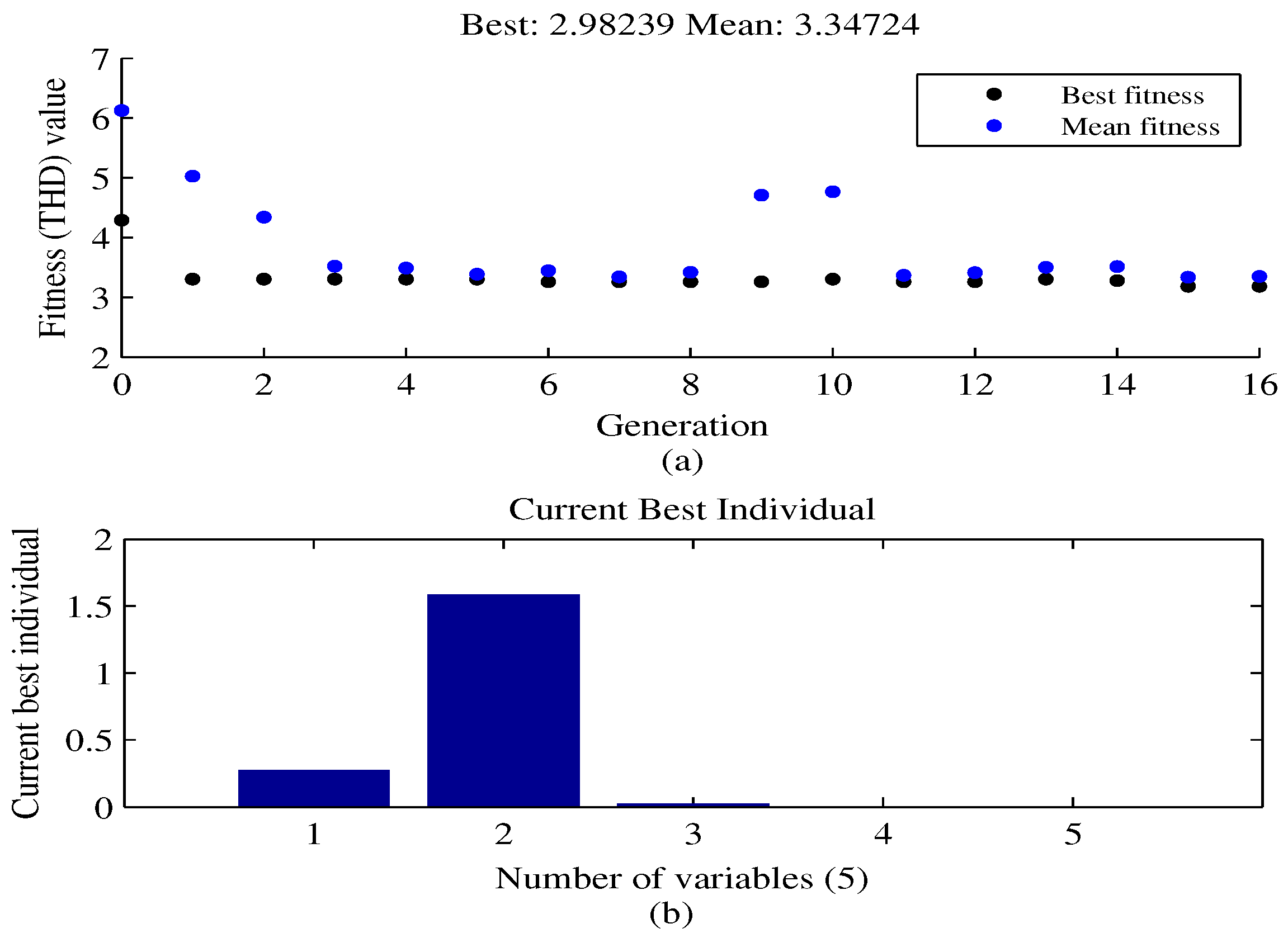
Figure 6 shows the optimization results obtained by the GA. Figure 6a represents the best and mean values of the filthiness function, i.e., the THD after each generation. In Figure 6a, we can observe the convergence of the THD with each generation. Figure 6b represents the optimum values of the individual parameters. As observed from GA optimization, we obtained optimum values of the parameters as R c = 25.4084 m Ω L c = 0.7738 mH, K p = 0.2623 K i = 1.5846 and C d c = 38.7848 μ F), as well as the lowest THD value of 2.98%.
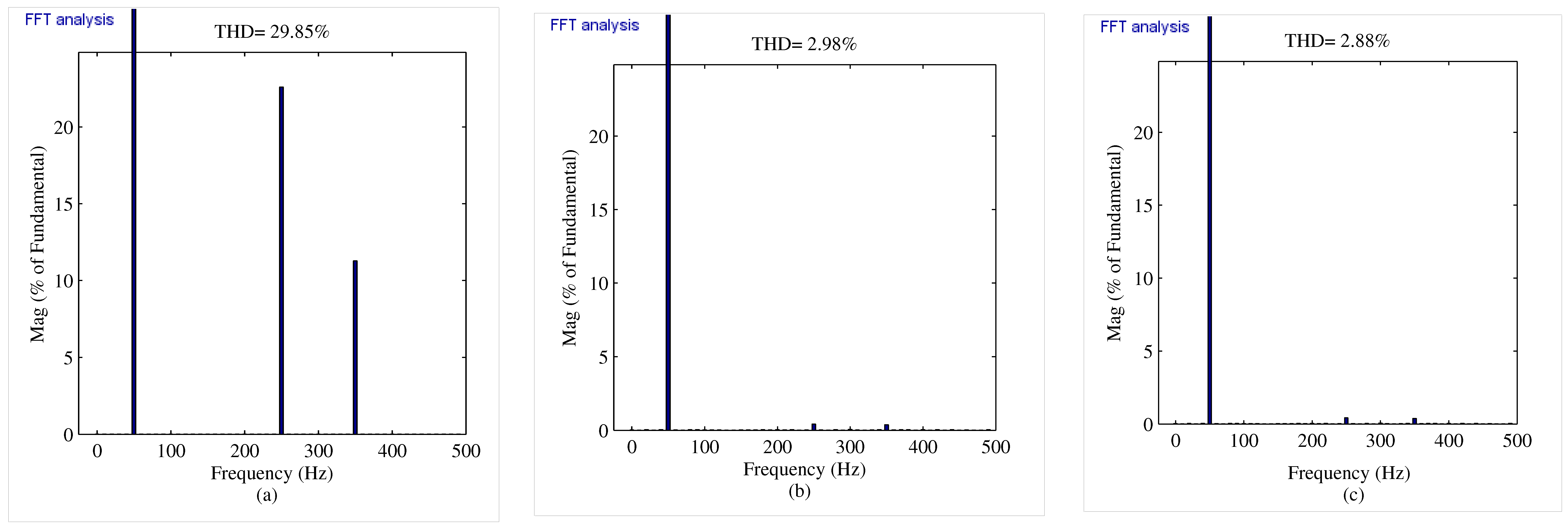
The simulation results for both the existing genetic algorithm method and the proposed Taguchi algorithm method are shown in 
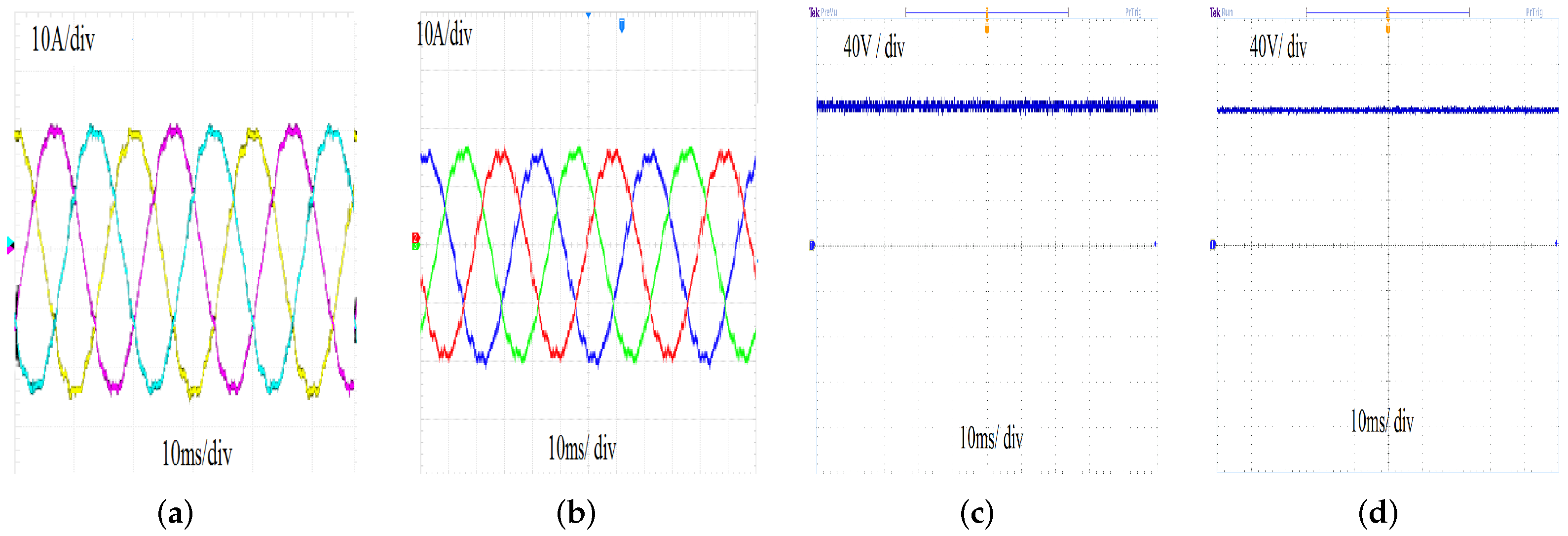
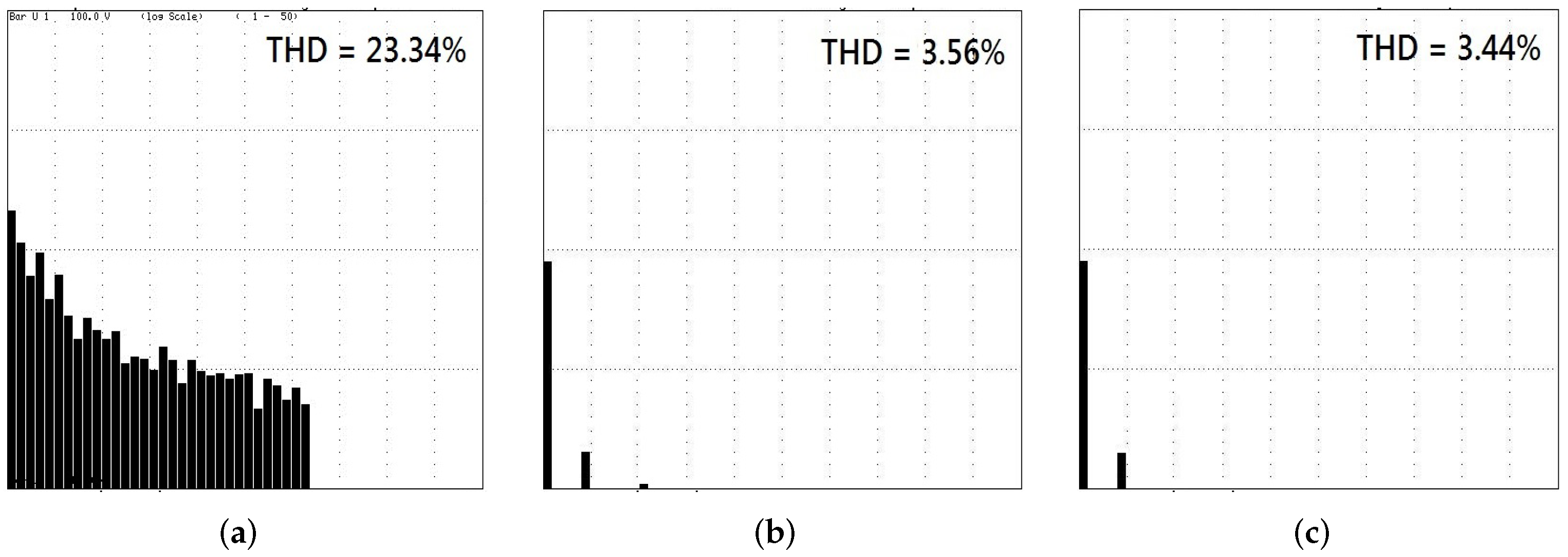
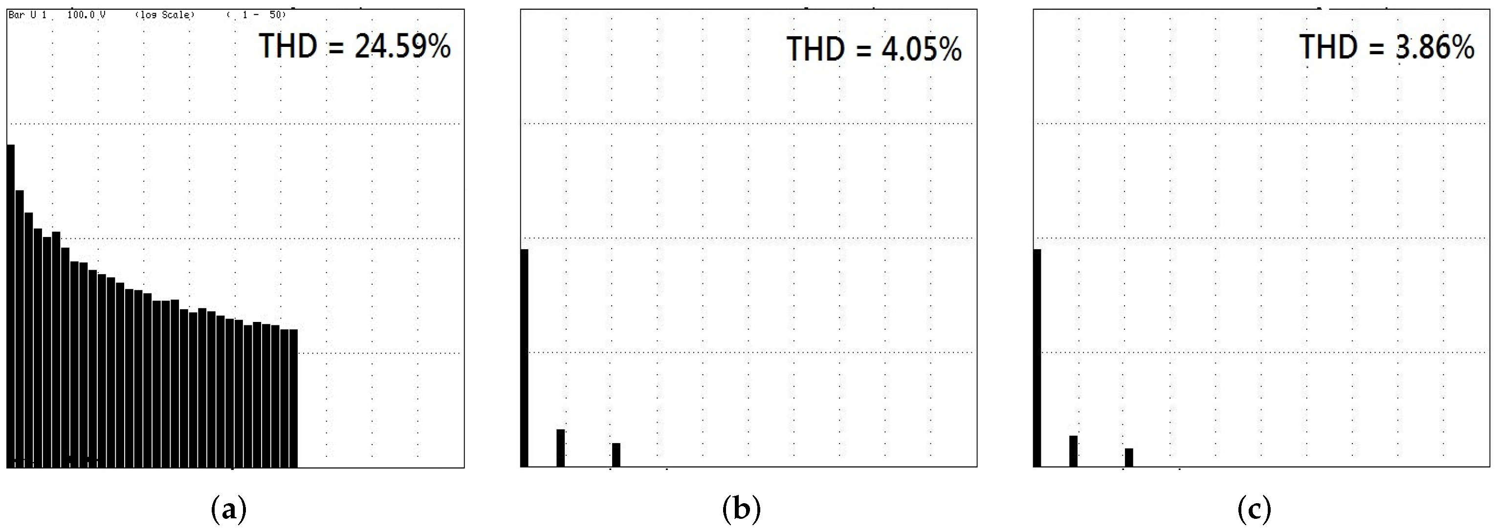
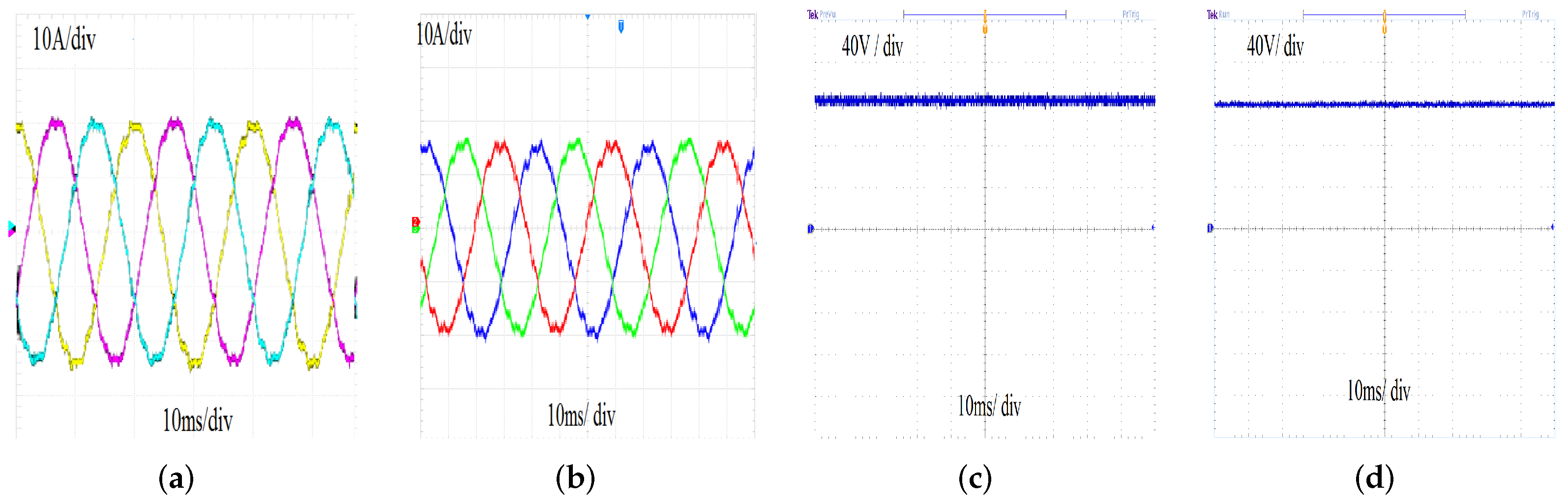
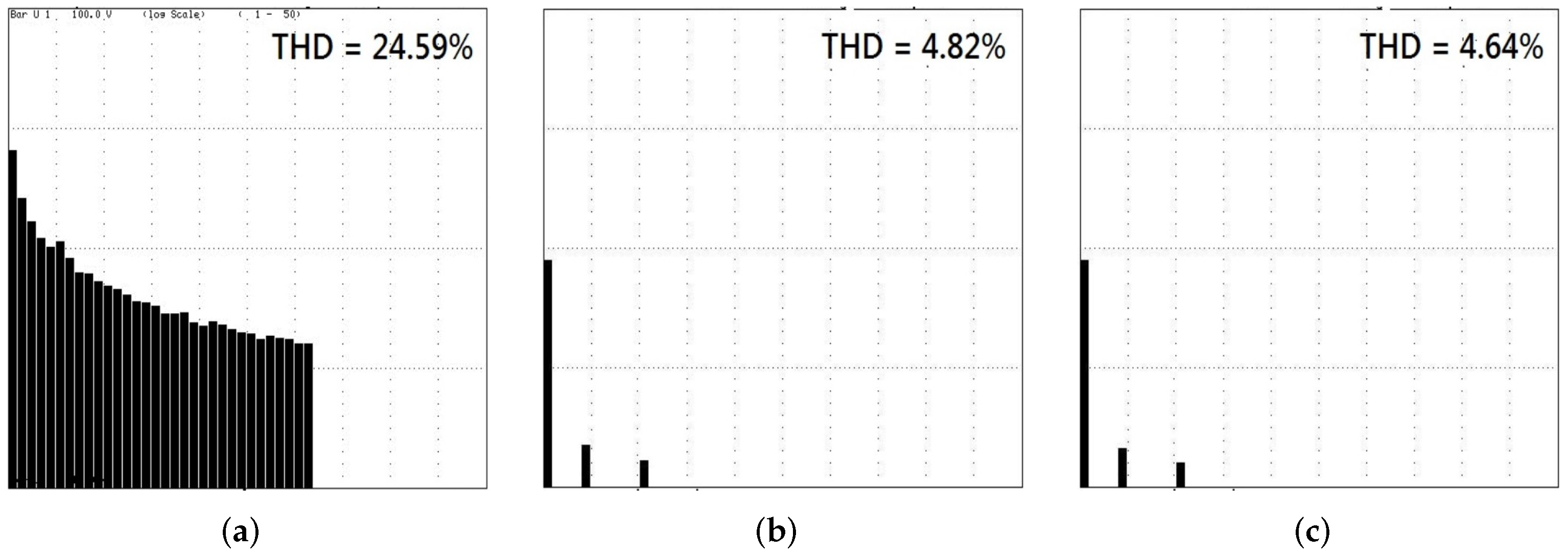
Figure 7. From the simulation results of the FFT analysis of the source current without compensation, the THD was 29.85%; with the proposed method’s compensation, the THD was reduced to 2.88%, which is lower than the existing genetic algorithm (THD = 2.98%). The superiority of the proposed method over the existing method was also verified by experimental validation with three different cases, mentioned below.

5. Experimental Results

The real validation of this proposed algorithm was implemented by a developed laboratory prototype. A DS1104 controller board was applied, which was very compatible with any version of MATLAB and was used for the controller design of the prototype. The control algorithm was developed on a dSPACE/MATLAB interactive common platform. The PWM signal was generated from the controller board passed to the SEMIKRON inverter. The hardware prototype developed in the laboratory included SIMICRON invertor, DS1104, voltage and current sensor and three-phase bridge rectifier as the non-linear load. The block diagram of the laboratory prototype is shown in Figure 8. Three-phase source voltage and load current are shown in Figure 9a,b, respectively. Figure 9c represents the three-phase filter current provided by the SAPF which compensates the harmonics in the source current. Table 6 represents the system parameters used for experimentation. The experimental analysis of the SAPF with the proposed algorithm is presented in the following subsections.

5.1. Case-I: Study of SAPF for Steady-State R-L Load Condition

The three-phase supply was connected to the three-phase bridge rectifier with an R-L (resistive–inductive) load, which injected harmonics into the distribution network. The three-phase source current after the application of the existing genetic algorithm and the proposed Taguchi method is shown in Figure 10a,b, respectively. It was observed that the source current was harmonic-free and sinusoidal. DC-link capacitor voltage for the existing and proposed methods is shown in Figure 10c,d, respectively. The THD before and after compensation for both the existing genetic algorithm and the proposed Taguchi method is shown in Figure 11. Without compensation, the THD was as high as 23.34%, as shown in Figure 11a. It was observed that the THD of the proposed Taguchi algorithm (THD = 3.44%) was lower than that of the existing genetic algorithm (THD = 3.56%). This is due to a better compensation of the proposed method over the existing method.

5.2. Case-II: Study of SAPF for Steady-State R-L-E Load Condition

In this case, a three-phase bridge rectifier with R-L-E (resistor–inductor–dc voltage source) was taken as the test load to verify the compensation capabilities of the SAPF. A 24 volt dc supply was connected in series with the existing R-L load. The three-phase source current after the application of existing genetic algorithm and the proposed Taguchi method is shown in Figure 12a,b, respectively. Figure 12c,d shows DC-link capacitor voltage for the existing and proposed methods, respectively. The THD of the load current is shown in Figure 13a. The THD of the source current with the existing and proposed methods is shown in Figure 13b,c. The load’s current harmonics were 28.59%. With the application of the proposed Taguchi algorithm, the THD was reduced to 3.86% compared with the existing genetic algorithm’s THD = 4.05%. Hence, the proposed algorithm enhanced the performance of the SAPF.

5.3. Case-III: Study of SAPF for Balanced Supply but Varying SAPF Parameter

In this case, the steady state of the SAPF parameters was changed to R c = 2 m Ω , L = 1.2 mH, V d c = 40 μ F. In this case, the validation of the proposed algorithm was verified compared with the existing algorithm. It can be noted, from Figure 14a,b, that the source current was better and the harmonics were fewer in the proposed algorithm as compared with the existing algorithm. Figure 14c,d shows DC-link capacitor voltage for the existing and proposed methods, respectively. The THD of the load current was 24.59%, as shown in Figure 15a. The source current THD for the proposed algorithm was 4.82%, which is better than the existing algorithm’s THD of 4.64%, as shown in Figure 15b,c, respectively. In all three considered cases, the proposed Taguchi algorithm method proved to be better than the existing genetic algorithm.
To measure the robustness performance of the SAPF, the harmonic compensation ratios (HRCs) were calculated and are shown in Table 6. The HCR is defined as the ratio of total harmonic distortion after and before compensation. It can be observed, from Table 6, that the proposed Taguchi algorithm provided less deviation in the HCR than the existing genetic algorithm.

6. Conclusions

In this paper, a new optimization algorithm method for SAPFs was implemented. The optimization algorithm is based on Taguchi’s signal-to-noise ratio (SNR). The Taguchi method for optimizing parameters reduces effort and time by decreasing the number of experiments. This method is simple, systematic and efficient to implement. With the application of this proposed method, the compensation performance of SAPF was enhanced as compared with the existing genetic algorithm, as demonstrated in the above simulation and experimental results of the various cases studied. Once again, Table 7 verifies the effectiveness of the proposed method over the existing method in terms of harmonic compensation ratio (HCR). From the HCR it is also clear that the proposed Taguchi method is superior to the existing genetic algorithm method for the optimization of the SAPF’s parameters. The Taguchi method also describes the rank of the parameters based on their effect on the results. The rank of the parameters defines the sensitivity of the parameters, which is not possible using the genetic algorithm.

Author Contributions

J.K.S., R.D.P. and S.D.S. devised the project and conceptualize the idea. R.T.N. and G.P. supervised the whole project. J.K.S. worked out technical details and performed the numerical calculations and simulation of the experiments. S.D.S. and J.K.S. obtained the experimental results for the project. The manuscript is drafted by J.K.S. and under the guidance of R.D.P., S.D.S., R.T.N. and G.P. All authors have read and agreed to the published version of the manuscript.

Funding

This research received no external funding.

Conflicts of Interest

The authors declare no conflict of interest.

References

  1. Akagi, H. New trends in active filters for power conditioning. Ind. Appl. 1996, 32, 1312–1322. [Google Scholar] [CrossRef] [Green Version]
  2. Hussien, Z.F.; Atan, N.; Abidin, I.Z. Shunt active power filter for harmonic compensation of nonlinear loads. In Proceedings of the National Power Engineering Conference, Bangi, Malaysia, 15–16 December 2003; pp. 117–120. [Google Scholar]
  3. Singh, B.; Al-Haddad, K.; Chandra, A. A review of active filters for power quality improvement. IEEE Trans. Ind. Electr. 1999, 46, 960–971. [Google Scholar] [CrossRef] [Green Version]
  4. Hoon, Y.; Radzi, M.; Amran, M.; Hassan, M.K.; Mailah, N.F. Control algorithms of shunt active power filter for harmonics mitigation: A review. Energies 2017, 10, 2038. [Google Scholar] [CrossRef] [Green Version]
  5. Angnlico, B.A.; Campanhol, L.B.G.; da Silva, S.A.O. Proportional–integral/proportional–integral-derivative tuning procedure of a single-phase shunt active power filter using Bode diagram. IET Power Electr. 2014, 7, 647–2659. [Google Scholar]
  6. Yamarthi, R.B.; Rao, R.S.; Reddy, P.L. Optimal load ompensation by shunt active power filter employing artificial bee colony optimization. In Proceedings of the 2016 International Conference on Electrical, Electronics, and Optimization Techniques (ICEEOT), Chennai, India, 3–5 March 2016; pp. 2197–2201. [Google Scholar]
  7. Kumar, R.; Chaturvedi, P.; Bansal, H.O.; Ajmera, P.K. Adaptive artificial neural network based control strategy for shunt active power filter. In Proceedings of the 2016 International Conference on Electrical Power and Energy Systems (ICEPES), Bhopal, India, 14–16 December 2016; pp. 194–199. [Google Scholar]
  8. Jogdand, V.V.; Panchade, V.M. Pi and Fuzzy Logic Based Shunt Apf for Power Quality Enhancement. In Proceedings of the 2016 International Conference on Electrical Power and Energy Systems (ICEPES), Bhopal, India, 14–16 December 2016; pp. 401–406. [Google Scholar]
  9. Hasanien, H.M.; Muyeen, S.M. A Taguchi approach for optimum design of proportional-integral controllers in cascaded control scheme. IEEE Trans. Power Syst. 2012, 28, 1636–1644. [Google Scholar] [CrossRef] [Green Version]
  10. Zanchetta, P.; Sumner, M.; Marinelli, M.; Cupertino, F. Experimental modeling and control design of shunt active power filters. Control Eng. Pract. 2009, 17, 1126–1135. [Google Scholar] [CrossRef]
  11. Thanh, H.P.; Van, H.D.; Duy, A.N.; Duy, C.N. Optimizing parameters of the shunt active power filter using Genetic algorithm. In Proceedings of the 2017 9th International Conference on Knowledge and Systems Engineering (KSE), Hue, Vietnam, 19–21 October 2017; pp. 233–238. [Google Scholar]
  12. Taguchi, G. Quality engineering (Taguchi methods) for the development of electronic circuit technology. IEEE Trans. Reliabil. 1995, 44, 225–229. [Google Scholar] [CrossRef]
  13. Rao, R.S.; Kumar, C.G.; Prakasham, R.S.; Hobbs, P.J. The Taguchi methodology as a statistical tool for biotechnological applications: A critical appraisal. Biotechnol. J. Healthc. Nutr. Technol. 2008, 3, 510–523. [Google Scholar] [CrossRef] [PubMed]
  14. Davis, R.; John, P. Application of Taguchi-Based Design of Experiments for Industrial Chemical Processes. Stat. Appr. Emph. Des. Exp. Appl. Chem. Process. 2018, 137. [Google Scholar] [CrossRef] [Green Version]
  15. Sorgdrager, A.; Wang, R.-J.; Grobler, A. Taguchi method in electrical machine design. SAIEE Afr. Res. J. 2017, 108, 150–164. [Google Scholar] [CrossRef] [Green Version]
  16. Athreya, S.; Venkatesh, Y.D. Application of Taguchi method for optimization of process parameters in improving the surface roughness of lathe facing operation. Int. Refer. J. Eng. Sci. 2012, 1, 13–19. [Google Scholar]
Figure 1. Configuration of SAPF.
Electronics 11 00348 g001
Figure 2. The reference current generation unit.
Electronics 11 00348 g002
Figure 3. PI controller for DC-link voltage regulation.
Electronics 11 00348 g003
Figure 4. Average of SNR for R c , L c , K p , K i and C d c .
Electronics 11 00348 g004
Figure 5. Optimization toolbox for implementing GA.
Electronics 11 00348 g005
Figure 6. GA simulation results (a) Optimized THD value (b) Optimized parameters values.
Electronics 11 00348 g006
Figure 7. (a) THD without SAPF. (b) THD with SAPF (existing method). (c) THD with SAPF (proposed method).
Electronics 11 00348 g007
Figure 8. Experimental setup.
Electronics 11 00348 g008
Figure 9. (a) Source voltage. (b) Load current. (c) Filter current.
Electronics 11 00348 g009
Figure 10. Case-I: Steady-state analysis with R-L load condition. (a) Source current in existing method. (b) Source current in proposed method. (c) DC-link capacitor voltage ( V d c ) for existing method. (d) DC-link capacitor voltage ( V d c ) for proposed method.
Electronics 11 00348 g010
Figure 11. Total harmonic distortion (THD) measurement for case-I. (a) THD without SAPF. (b) THD with SAPF (existing method). (c) THD with SAPF (proposed method).
Electronics 11 00348 g011
Figure 12. Case-II: Steady-state analysis with R-L-E load condition. (a) Source current in existing method. (b) Source current in proposed method. (c) DC-link capacitor voltage ( V d c ) for existing method. (d) DC-link capacitor voltage ( V d c ) for proposed method.
Electronics 11 00348 g012
Figure 13. Total harmonic distortion (THD) measurement for case-II. (a) THD without SAPF. (b) THD with SAPF (existing method). (c) THD with SAPF (proposed method).
Electronics 11 00348 g013
Figure 14. Case-III: Study of SAPF for balanced supply but varying SAPF parameter. (a) Source current in existing method. (b) Source current in proposed method. (c) DC-link capacitor voltage ( V d c ) for existing method. (d) DC-link capacitor voltage ( V d c ) for proposed method.
Electronics 11 00348 g014
Figure 15. Total harmonic distortion (THD) measurement for case-III. (a) THD without SAPF. (b) THD with SAPF (existing method). (c) THD with SAPF (proposed metod).
Electronics 11 00348 g015
Table 1. SAPF parameters and their levels.
ParametersLevel 1Level 2Level 3Level 4
R c 0.1 m Ω 1 m Ω 10 m Ω 100 m Ω
L c 0.5 mH1 mH1.5 mH2 mH
K p 0.010.050.100.50
K i 0.010.1110
C d c 10 μ F20 μ F30 μ F40 μ F
Table 2. Experimental matrix.
Exp. No. R c (m Ω ) L c (mH) K p K i C d c ( μ F ) THD in %
10.10.50.010.01107.55
20.110.050.1203.11
30.11.50.11306.43
40.120.510407.88
510.50.051405.98
6110.0110302.97
711.50.50.01207.23
8120.10.1109.56
9100.50.110207.55
101010.51103.31
11101.50.010.1406.62
121020.050.01309.55
131000.50.50.1305.29
1410010.10.01403.86
151001.50.0510104.71
1610020.011209.94
Table 3. Signal-to-noise ratio (SNR).
Experiment NoSignal-to-Noise Ratio ( η ) in dB
1−17.5589
2−9.85521
3−16.1642
4−17.9305
5−15.534
6−9.45513
7−17.1828
8−19.6092
9−17.5589
10−10.3966
11−16.4172
12−19.6001
13−14.4691
14−11.7317
15−13.4604
16−19.9477
Table 4. Average SNR for individual factors and each level.
Level R c L c K p K i C d c
1−15.38−16.28−15.84−16.52−15.26
2−15.45−10.36−14.61−15.09−14.16
3−15.99−15.81−14.27−15.51−14.92
4−14.90−19.27−14.99−14.60−14.40
Sum of
Difference
1.098.911.651.921.21
Rank51324
Table 5. Optimum levels of factors and their values.
ParameterOptimum LevelOptimum Value
R c 4100 m Ω
L c 21 mH
K p 20.05
K i 410
C d c 330 μ F
Table 6. System parameters for experimentation.
System ParametersValues
Supply Voltage and Frequency V s = 100 V, f = 50 Hz
Line Impedance R s = 0.10 Ω , L s = 0.5 mH
Load Impedance R l = 100 Ω , L l = 40 mH, E = 24 V
Table 7. Harmonic compensation ratio (HCR).
CasesTHD (in %) of Source CurrentHCR (in %)
Before CompensationAfter Compensation
Case-IExisting23.343.5615.25
Proposed23.343.4414.73
Case-IIExisting24.594.0516.47
Proposed24.593.8615.69
Case-IIIExisting24.594.8619.60
Proposed24.594.6418.86
Publisher’s Note: MDPI stays neutral with regard to jurisdictional claims in published maps and institutional affiliations.

