Article

Space Discretization-Based Optimal Trajectory Planning for Automated Vehicles in Narrow Corridor Scenes

1
State Key Laboratory of Advanced Design and Manufacturing for Vehicle Body, College of Mechanical and Vehicle Engineering, Hunan University, Changsha 410082, China
2
Wuxi Intelligent Control Research Institute, Hunan University, Wuxi 214115, China
*
Author to whom correspondence should be addressed.
Electronics 2022, 11(24), 4239; https://doi.org/10.3390/electronics11244239
Submission received: 16 November 2022 / Revised: 14 December 2022 / Accepted: 15 December 2022 / Published: 19 December 2022
(This article belongs to the Special Issue Recent Advances in Motion Planning and Control of Autonomous Vehicles)

Abstract

:
The narrow corridor is a common working scene for automated vehicles, where it is pretty challenging to plan a safe, feasible, and smooth trajectory due to the narrow passable area constraints. This paper presents a space discretization-based optimal trajectory planning method for automated vehicles in a narrow corridor scene with the consideration of travel time minimization and boundary collision avoidance. In this method, we first design a mathematically-described driving corridor model. Then, we build a space discretization-based trajectory optimization model in which the objective function is travel efficiency, and the vehicle-kinematics constraints, collision avoidance constraints, and several other constraints are proposed to ensure the feasibility and comfortability of the planned trajectory. Finally, the proposed method is verified with both simulations and field tests. The experimental results demonstrate the trajectory planned by the proposed method is smoother and more computationally efficient compared with the baseline methods while significantly reducing the tracking error indicating the proposed method has huge application potential in trajectory planning in the narrow corridor scenario for automated vehicles.

1. Introduction

Automated vehicles have drawn a huge amount of attention from academia and industry in recent years because of the foreseen potential to improve driving safety and efficiency [1,2,3]. With researchers’ continuous efforts, autonomous driving technologies have made great progress over the past few decades [4,5,6,7]. However, as one of the core modules in an autonomous vehicle system, trajectory planning remains to be challenging, especially in complicated environments. Narrow corridors are typically among the most complicated scenes, in which generating a safe, feasible, and smooth trajectory is difficult due to the exterior and interior restrictions.

1.1. Related Work

Numerous studies have been devoted to vehicle trajectory planning [8,9,10,11]. The mainstream methods in these studies can be classified into four groups: curve interpolation methods, sampling methods, graph search methods, and numerical optimal control methods [12]. The curve interpolation methods generate a trajectory by interpolating the waypoints in a known set with curves such as the RS curve, clothoid, polynomial, Bezier, B-spline, and so on [13]. For example, in [14], Bae et al. adopted a quintic Bezier curve to generate candidate paths in the lane change maneuver while using lateral acceleration as the path judgment index. Sampling methods try to search for the connectivity of the configuration space by randomly sampling knots in it [15]. Rapid-exploring Random Tree (RRT) is the most typical sampling-based method. For example, in [16], Zheng et al. applied RRT to autonomous parking with vehicle nonholonomic constraints considered. The aforementioned two categories of methods are easy to implement, yet they are not applicable in complicated environments. In detail, paths generated by curve interpolation are deeply influenced by the preset waypoints, while paths generated by randomly sampling are not consistent. Moreover, paths generated by these two methods are suboptimal. Instead, graph search methods could construct the optimal trajectory by traversing the entire state space to find paths with the minimum cost [17]. One famous algorithm of graph search-based methods is the A* algorithm. For example, in [18], Min et al. proposed an improved A* algorithm in an unstructured environment, in which profile collision avoidance was realized by simply setting a redundant security space. Graph search-based methods are inefficient while being used in high-dimensional spaces. To improve this method, some researchers combined the graph search methods with the former curve interpolation methods or sampling methods. In [19], Li et al. used the RS curve and the hybrid A* algorithm to generate paths for automatic parking, yet the path is not curvature continuous. In [20], Dirik and Kocamaz proposed an RRT-Dijkstra algorithm to plan paths with discontinuous curvature. Although graph search methods could construct the optimal trajectories, they could not directly deal with complicated constraints such as obstacle avoidance and actuator limitation. Conversely, optimization-based methods could construct an optimal trajectory while well handling complicated constraints by creating accurate mathematical models [21]. In [22], Li et al. designed a moving trend function in a framework of nonlinear model predictive control, using a risk index to realize collision avoidance. In [23], Dixit et al. used an MPC controller to generate feasible and collision free trajectories by combing the artificial potential field method. In [24], Zhu et al. constructed an optimization problem of parameterized curvature control to realize trajectory generation in dynamic on-road driving environments. Though the trajectories generated by these optimization-based methods are feasible, smooth, and continuous, even in complicated environments, yet they are computational complex.
Narrow corridors are a special but common working scene for vehicles, especially for special purpose vehicles working in a fixed route. These vehicles include logistics vehicles in parks, forklifts in warehouses, underground scrapers in mines, and so on. Passable areas of those vehicles in narrow corridors are strictly limited by the corridor boundaries. Thus, vehicle motion in narrow corridors should be as precise as possible, otherwise, vehicles could collide with the corridor boundaries or could not pass the turning areas. Existing studies on trajectory planning for narrow corridors are concentrated on mobile robots such as unmanned aerial vehicles, and sampling-based methods are the most popular [25]. However, unlike those mobile robots with holonomic constraints who could perform in situ steering, vehicle turning maneuvers are restricted by the non-holonomic vehicle kinematics constraints. Thus, sampling-based methods, whose trajectory curvature is not continuous, are not suitable for vehicle trajectory planning in narrow corridors. There are a few studies on vehicle trajectory planning in narrow passable areas. In [26], Kim et al. used Dubins curves to generate paths for narrow parking lots in a predefined collision-free space, in which curvature of the generated path is discontinuous and quite a part of accessible areas is sacrificed. In [27], considering the parking environment with uncertainty, Li et al. proposed a parallel stitching strategy to replan the trajectory for avoiding the new appeared obstacles utilizing the accessible areas. In [28], Do et al. proposed a method based on the support vector machine (SVM) and fast marching method (FMM) to plan paths for narrow passage, in which obstacle avoidance and vehicle kinematics were considered yet other constraints such as vehicle actuator limitation and terminal postures were ignored. In [29], Tian et al. explored a method about how to turn around in narrow environments, in which RS curves and Bezier curves were applied. With RS curves, a lot of free space would be occupied in the place where the forward and back segments meet. Therefore, this method would not be applicable in a strictly restricted narrow corridor. In [30], Li et al. proposed a progressively constrained strategy that solves a sequence of easier planning problems with shrunk obstacles before handling their nominal sizes. Although the finally derived trajectories are curvature-continuous and optimal, the runtime is usually long and the algorithm performance relies highly on the initial guess. In [31], with the aim of reducing computational time, Li et al. proposed a lightweight iterative framework to generate an optimal trajectory for autonomous parking. In [32], Lin et al. proposed a trajectory planning method for the mine scene but the experiments were not convincing due to the lack of field tests. Methods mentioned above do generate collision-free paths in narrow area scenes. However, the studies above either only consider the trajectory property of collision avoidance or aim at totally different subject models and vehicle operation space, which restricts their application in the narrow corridor scene.

1.2. Contributions

In this paper, we extend our previous work [32] in terms of successfully applying the space discretization-based optimal trajectory planning method (hereinafter called the SOTP method) for automated vehicles in multi-corner narrow corridor scenes, wherein the trajectory curvature is guaranteed to be continuous, every inch of the precious drivable space is sufficiently utilized, and exterior/interior constraints are strictly satisfied. In the proposed SOTP method, we first design a mathematically-described driving corridor and discretize its centerline to generate reference waypoints. Based on these derived reference waypoints, we thereafter formulate a trajectory optimization model in the spatial domain with the consideration of travel time minimization, boundary collision avoidance, and constraint satisfaction in terms of vehicle kinematics, actuator range limitation, side force, etc. Finally, the constructed trajectory optimization model is verified with both simulations and field tests. The main contributions of this paper are as follows:
(1) A novel space discretization-based optimization method is proposed to solve the challenging trajectory planning problem in narrow corridor scenes with very limited passable areas. Compared with [32], more complicated constraints, e.g., boundary avoidance is considered and processed with the accurately established mathematical models of the vehicle and the narrow corridor being embedded into the trajectory generation process.
(2) A space discretization strategy is designed for the construction of the trajectory optimization model. In this strategy, we consider the target trajectory to be described by several discrete waypoints with velocity information. The simulation is designed to demonstrate the enhanced smoothness and computational efficiency of the trajectory planned by the proposed method compared with the baseline algorithm. A sensitivity analysis of the key parameter, e.g., the safety margin is conducted to show the performance of the proposed method.
(3) The field tests related to the trajectory generation ability and the quality of the generated trajectory are conducted to illustrate the advantages of the proposed method over a popular method in the application of the narrow corridor scenes.

1.3. Organization

The rest of this paper is organized as follows. Section 2 formulates the problem. Section 3 introduces the methodology. Section 4 and Section 5 present the simulation and field test results respectively. Finally, Section 6 concludes the paper.

2. Problem Statement

Narrow corridors concerned in this paper refer to one-way roads with the ratio of vehicle width to road width exceeding 0.5. The workspace for vehicles operating in such corridors is usually closed and fixed, which brings a challenge for trajectory generation. In this case, how to generate such a reference trajectory is exactly what we explore below. We assume that the boundary and the centerline of the narrow corridor could be accessible by the perception technology or high definition map.
We consider a typical narrow corridor with specified left and right boundaries. Since the twisted narrow corridor makes it difficult for a vehicle to traverse, we simplify the boundaries via line segments and assume the corridor to be straight (Figure 1). By linear interpolation of the boundary position, we describe the corridor mathematically by using the formulas as follows:
A i l x + B i l y + C i l = 0 ,
A i r x + B i r y + C i r = 0 ,
where A i l , B i l , C i l are expression parameters of the left boundary in segment i and A i r , B i r , C i r are the right boundary. Suppose the corridor is comprised of N s segments, so i ranges from 1 to N s .
In the process of passing the narrow corridor, the vehicle is expected to run smoothly and efficiently without any collisions. Therefore, the reference trajectory which the automated vehicle tries to track should be smooth, efficient, and collision-free under the premise of feasibility. To generate such a trajectory, several factors are considered. In detail,
(1) For smoothness, large side-force related to high speed and large curvature is avoided, and the vehicle posture at the corridor terminal is restricted and the motion parameters are limited.
(2) For efficiency, the travel time is minimized.
(3) For collision avoidance, obstacle avoidance conditions based on the circle-fitting strategy are designed.
(4) For feasibility, trajectory generation is set up upon vehicle kinematics and the trajectory is designed as per the actuator range.

3. Methodology

To generate a time-optimal trajectory for a narrow corridor, we explore the trajectory optimization model as follows.

3.1. Vehicle Kinematics Modeling

Vehicles in a narrow corridor generally travel with a low or medium speed because of safety concerns, so the vehicle kinematic model [33], i.e., the bicycle model (Figure 2) that satisfies Ackerman’s steering principles, is capable here.
Similar to [32], we use the coordinate of the rear axle center to represent the vehicle position. With the above-mentioned kinematic model, the vehicle kinematic equations generally expressed in the time domain are as follows:
x ˙ = v cos ( φ ) ,
y ˙ = v sin ( φ ) ,
φ ˙ = v tan ( α ) L ,
where x and y are the vehicle position in the global coordinate system, φ is the vehicle yaw angle, v is the velocity, α is the steering angle and L is the wheelbase.
In this study, we discuss the trajectory planning problem in the space domain to make better use of the position information of the corridor boundaries. Therefore, we transform the kinematic relationship from the time domain to the space domain with the chain rule d ( · ) d t = d ( · ) d s d s d t = v d ( · ) d s . The transformed kinematic equations are as follows:
x = d x d s = x ˙ v = cos ( φ ) ,
y = d y d s = y ˙ v = sin ( φ ) ,
φ = d φ d s = φ ˙ v = tan ( α ) L ,
where x and y are the first derivatives of the vehicle position versus space, and φ is the first derivative of the vehicle yaw angle versus space.

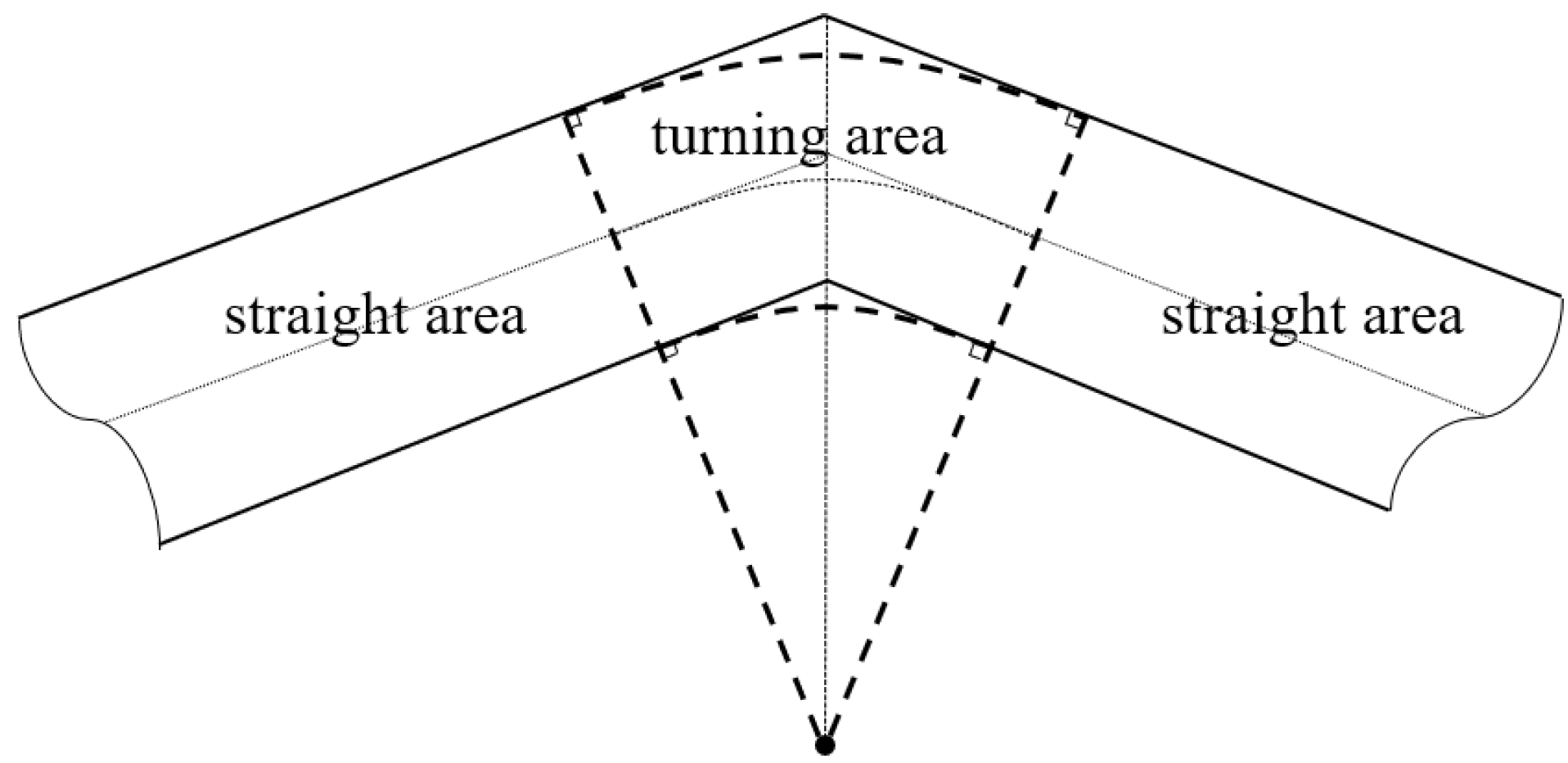
3.2. Space Discretization Strategy

In narrow corridors, the total travel time is unpredictable due to the unknown velocity. On the contrary, the total travel distance can be approximated by the corridor centerline due to the limited drivable area. Particularly, the approximation error is tiny between the corridor centerline discrete interval and the target trajectory discrete interval. Therefore, we design a space discretization strategy here to construct the trajectory optimization model. In detail, we take the discrete waypoints on the corridor centerline as a reference and use its discrete interval to approximate the target trajectory discrete interval. In this way, the mathematical relationships in the target trajectory can be explicitly described and the target trajectory can be directly solved.
In the space discretization strategy, we discretize the vehicle trajectory in the space domain and describe the trajectory by the discrete waypoints with velocity information. To provide reference waypoints for this discrete trajectory, we discretize the corridor centerline with certain rules. For the reason that vehicle operation in corner areas is more difficult than that in other areas, we deal with these two situations differently by dividing the corridor into turning areas and straight areas. In this process, the turning area is decided by the unique tangent points of the corridor boundaries and corridor turning arcs with a fixed corridor turning center, see Figure 3. Then, we discretize the centerline in the turning areas and the straight areas separately, see Figure 4. The discrete points in the turning areas are expected to be denser than the discrete points in the straight areas because of the much harder driving environment in the turning areas. Thus, the waypoint interval in the turning areas should be smaller than that in the straight areas. With the rules mentioned above, we discretize the corridor centerline into N waypoints and then record their position information. Here x o ( k ) , y o ( k ) , k = 1 , 2 , , N is used to represent the waypoint position in the global system and Δ s ( k ) , k = 1 , 2 , , N 1 is used to represent the waypoint interval.
Now that the reference centerline has been discretized into N waypoints, the target trajectory can be approximated by these N points in the form of ξ ( s ( k ) ) = ξ ( s ( 1 ) ) + j = 1 k 1 Δ s ( j ) , k = 2 , 3 , , N , in which target trajectory waypoints interval are replaced by the centerline waypoint interval Δ s ( k ) . We choose the vehicle position, vehicle yaw angle, and vehicle velocity as the trajectory states. Thus, the final target trajectory ξ ( s ( k ) ) can be represented by a sequence X ( k ) , k = 1 , 2 , , N as follows:
X ( k ) = [ x ( k ) , y ( k ) , φ ( k ) , v ( k ) ] .
What should be noted here is that the final trajectory would be approximate because the actual intervals of the target trajectory waypoints are approximated by the centerline waypoint intervals to express mathematical relationships explicitly and to directly plan the target trajectory. Moreover, the approximation strategy used here is reasonable and workable for the reason that the error caused by this strategy is very small in the case of a narrow corridor.

3.3. Vehicle Trajectory Optimization

This subsection presents the construction of the trajectory optimization model based on the space discretization strategy, considering the constraints related to safety, feasibility, smoothness, and travel time.

3.3.1. Objective Function

Concerns about vehicle trajectory planning are mainly concentrated on safety, feasibility, comfort, and efficiency. The first three ones are hard constraints, while the efficiency requirement is a soft one. Thus, we choose efficiency as the objective here, and an objective function based on the corridor travel time is designed. By taking the discrete waypoints as a reference, the total travel time can be approximately expressed as:
J = k = 1 N 1 Δ s ( k ) v ( k ) .

3.3.2. Terminal Posture Constraints

The vehicle positions in the corridor entrance and exit are expected to be on the corridor centerline, while the vehicle yaw angles are expected to be parallel to the corridor heading orientations, which makes it quite difficult to find an exact solution. Thus, we constrain the vehicle’s final state to be near the expected posture. By taking the discrete waypoints as a reference, the terminal constraint can be expressed as:
x ( 1 ) = x o ( 1 ) , x ( N ) = x o ( N ) ± Δ x ,
y ( 1 ) = y o ( 1 ) , y ( N ) = y o ( N ) ± Δ y ,
φ ( 1 ) = θ enter , φ ( N ) = θ exit ± Δ θ ,
where θ enter and θ exit are the orientations of the corridor entrance and exit. The sizes of Δ x , Δ y , Δ θ are expected to be appropriate to guarantee that the vehicle is within the corridor.

3.3.3. Vehicle Kinematics Constraints

Vehicle operation follows the kinematics relationship. Hence, the vehicle kinematics constraints are considered here. By taking the discrete waypoints as a reference, the kinematics constraints in the space domain can be approximately expressed as follows:
x ( k + 1 ) = x ( k ) + Δ s ( k ) cos ( φ ( k ) ) ,
y ( k + 1 ) = y ( k ) + Δ s ( k ) sin ( φ ( k ) ) ,
φ ( k + 1 ) = φ ( k ) + Δ s ( k ) tan ( φ ( k ) ) L .

3.3.4. Vehicle Speed Constraints

We consider the constraint of vehicle speed here. By taking the discrete waypoints as a reference, the vehicle speed constraint is as follows:
v min v ( k ) v max .

3.3.5. Actuator Range Constraints

There are both longitudinal and lateral actuator constraints in a vehicle’s operations. We ignore the limitation of longitudinal actuators here for the fact that a vehicle’s normal operation in a narrow corridor would never reach its acceleration/deceleration limits. Though the longitudinal actuator limitation is ignored here, we would restrict the longitudinal motion parameters for comfort. This would be discussed in a later subsection. For the later actuator, its range could not be ignored since an adequate steering angle is necessary in a narrow turning area. By taking the discrete waypoints as a reference, the constraint of steering is as follows:
α max α ( k ) α max .

3.3.6. Tire Side-Force Constraints

A big tire slip angle caused by a large side force would lead to vehicle model invalidation. To avoid this situation, the side force related to the vehicle speed and path curvature is constrained by the formula v 2 R μ g , where R is the curvature radius, μ is the side-force coefficient, and g is the gravity coefficient. Since the vehicle follows the Ackerman steering principle, R is dependent on the formula R = L tan ( α ) . By taking the discrete waypoints as a reference, the final expression of the side-force avoidance constraint is as follows:
v ( k ) 2 tan ( α ( k ) ) L μ g .

3.3.7. Acceleration and Angular Velocity Constraints

Motion change has a great influence on the smoothness and comfort of vehicle operation. The vehicle motion is realized by speed control in the longitudinal direction and front steering control in the lateral direction. Thus, we consider constraining the change of the speed and steer angle here. That is to say, we constrain the acceleration and steer angular velocity. Since we take the discrete waypoints as a reference, the constraints can be approximately expressed as:
v 2 ( k + 1 ) v 2 ( k ) 2 Δ s ( k ) a max ,
v ( k ) ( α ( k + 1 ) α ( k ) ) Δ s ( k ) ω max ,
where a max represents the limit value of accleration and ω max represents the limit value of the steering angle velocity.

3.3.8. Collision Avoidance Constraints

Safety is the most important consideration in vehicle trajectory planning. For narrow corridor scenarios, safety means no border collision happens. For border-collision detection, we adopt a strategy of approximating a vehicle body shape with circles here to describe the collision condition intuitively and leave some safety margin at the same time [34], as shown in Figure 5.
In the circle fitting strategy, the circle parameters are decided by the circle number and vehicle body parameters. Suppose the vehicle is fitted by N c circles, and then the circle’s parameters are calculated as follows:
x j c ( k ) = x ( k ) + ( l f + L + l N c ( 0.5 j ) cos ( φ ( k ) ) ,
y j c ( k ) = y ( k ) + ( l f + L + l N c ( 0.5 j ) sin ( φ ( k ) ) ,
r = 0.5 ( l N c ) 2 + w 2 ,
where r is the circle radius, x j c ( k ) , y j c ( k ) are the circle center position of the j th fitted circle, L is the wheel base, l and w are the length and width of the vehicle respectively.
Now that the circle centers and radius are quantitatively derived. Boundary-collision detection can be easily realized by comparing the value of the circle radius with all the distance from the circle centers to the corresponding boundary segments, as shown in Figure 6.
If any distance is less than the circle radius, a collision between the vehicle and corridor boundary happens. Therefore, all the distances should be greater than the circle radius. In particular, the distance between a circle center and the boundary segments is as follows:
d j l ( k ) = A i l x j c ( k ) + B i l y j c ( k ) + C i l A i l 2 + B i l 2 ,
d j r ( k ) = A i r x j c ( k ) + B i r y j c ( k ) + C i r A i r 2 + B i r 2 .
By taking the discrete waypoints as a reference, the collision avoidance constraints can be expressed as:
A i l x j c ( k ) + B i l y j c ( k ) + C i l 2 r 2 A i l 2 + B i l 2 > 0 ,
A i r x j c ( k ) + B i r y j c ( k ) + C i r 2 r 2 A i r 2 + B i r 2 > 0 ,
in which k range from 1 to N. On the basis of [32], the principle of the parameter and its influence on the results will be discussed in Section 4.3.

3.4. SOTP Method Design

With the objective function and the constraints mentioned above, the trajectory optimization model is finally constructed as follows:
min ( 10 ) , s . t . ( 11 ) to ( 21 ) , ( 27 ) to ( 28 ) .
The trajectory optimization model would lead to an optimal sequence of vehicle velocities and steering angles. By the integration of this sequence, a target trajectory with the characteristics of safety, feasibility, comfort, and efficiency would finally be generated.
What should be noticed here is that the target trajectory is used for reference in a fixed scene. Thus, the optimization model is solved in a single time rather than the rolling horizon way. Moreover, if the solving process fails to find an optimal solution because of being trapped in a local infeasibility point, a trajectory recorded by an experienced driver could be used to replace the target trajectory.

4. Numerical Simulation

Numerical simulation is conducted to verify the proposed SOTP method. We first test the practicability in the single corner scenario and subsequently conduct statistical analysis in the narrow corridor scenario with multi-corners compared with the baseline methods.

4.1. Single Corner Scenario

Narrow corridors are hard for vehicles to pass because the corridor boundaries strictly limit the collision-free space, especially in the turning area. Therefore, in this subsection, we apply the proposed method SOTP to the single corner scenario for investigating two problems: (1) could the proposed method be feasible for the narrow corridor scene with single corner? (2) what is the minimum corridor turning angle for passing?

4.1.1. Simulation Setup

To explore the solving ultimate limitation of the proposed method SOTP, we here construct a narrow corridor cluster with a decreasing amplitude of 5 , which ranges from 180 to the minimum angle within their solving capability. Parameters of the narrow corridor cluster are shown in Table 1. As for the vehicle model and vehicle motion limitation, we adopt the same parameters as in Table A2 and Table A3 respectively. As we construct terminal posture constraints, we need to set the threshold value Δ x , Δ y , Δ θ to ensure the vehicle’s final posture to be near the expected posture. The key parameters of the SOTP method are all listed in Table 2.
We use the platform of MATLAB to design the mathematically-described narrow corridors and establish the proposed trajectory generation model. Since the trajectory planning process discussed in this paper is converted to a nonlinear program (NLP), we here use the NLP solver, IPOPT [35], to find the solution. After realizing trajectory generation by the SOTP method, we subsequently set the trajectory tracking simulation on a co-simulation platform of Simulink and CarSim to prove the generated trajectory could be tracked in the practical application. For the established tracking controller, we take the famous Stanley algorithm [36] for lateral tracking and the classical PID algorithm for longitudinal tracking. All processes are executed on an Intel Core i5-11300H CPU with 16 GB RAM that runs at 3.1Ghz.

4.1.2. Simulation Result

The minimum corner angle required to find a feasible solution is 120 for the proposed SOTP method. As for the study purpose of this subsection, we here choose five groups of data from the corridor clusters, within which the solvability of our method is guaranteed, to illustrate the proposed method’s performance. These five groups of data belong to Narrow Corridor NC1, Narrow Corridor NC4, Narrow Corridor NC7, Narrow Corridor NC10 and Narrow Corridor NC13 of which the corner angles are 180 , 165 , 150 , 135 and 120 .
As shown in Figure 7, the planned trajectory is smooth with the guarantee of minimum travel time and collision free. With the decrease in the turning angle, the average velocity of the trajectory slow down as well while the controller could track the generated trajectory which indicates the proposed method has huge potential to solve the narrow corridor scenario.

4.2. Multi Corners Scenario

In this subsection, we apply the proposed method and the baseline methods to a more general scenario that has two corners and evaluate the quality of the generated trajectories according to the evaluation metrics to present the excellent performance of the proposed method. The narrow corridor scenario with limited collision-free space means the scope of the feasible solution is smaller compared with those scenes with a larger passable area. Hence, we only consider the narrow corridor scenario.

4.2.1. Baseline Methods

The baseline algorithm we choose for comparison is the hybrid state A* algorithm and dynamic window approach (DWA) method [37]. The hybrid state A* method is widely used in complicated scenes because of its advantage to find the optimal path satisfying the non-holonomic constraints while the DWA method is popular in mobile robot navigation by generating the control variables directly to avoid obstacles.
In the hybrid state A* algorithm, the path is formed by extending the nodes on the grid map with the lowest cost in the 3D kinematic state space. Since the extending nodes are influenced by the grip resolution, the target posture may never be reached. In this case, a termination condition is necessary so that the search process can be stopped once the extending node reaches a preset domain. In this study, we set the domain as: Δ x : ± 0.25 m , Δ y : ± 0.25 m , Δ φ : ± 15 After finishing the search process, a rough path can be formed. Since the curvature of the original path is not continuous, a smoothing process is essential. We use the conjugate gradient descent algorithm introduced in [38] to smooth the original path here. Besides path planning, vehicle velocity also needs to be planned. Based on the path generated by the hybrid A* algorithm, we here adopt nonlinear programming to plan the vehicle velocity, considering the side force and acceleration constraint.

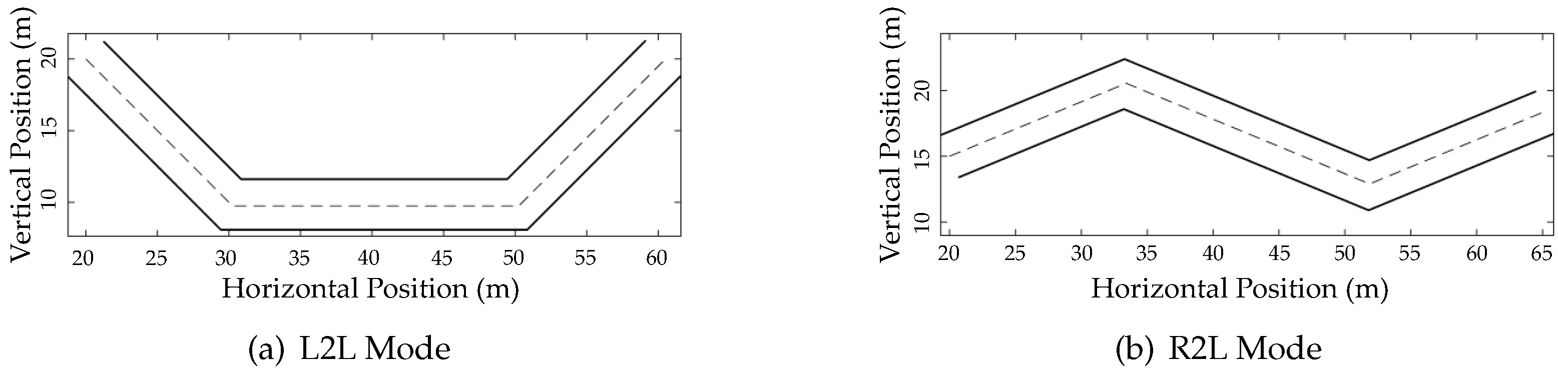
4.2.2. Simulation Setup

In this case study, the narrow corridor scenarios with more than two corners could be split into a scene with two corners. Therefore, we only consider two special narrow corridors. The first narrow corridor turns continuously in the same direction, while the second turns continuously in the opposite direction. The former situation can be continuous left to left turns or right to right turns. We name them the L2L mode and the R2R mode. The latter situation can be continuous right to left turns or left to right turns. We name them the R2L mode and the L2R mode. Because of the symmetry, we only need to simulate one mode in each situation. As shown in Figure 8, narrow corridors with the L2L and R2L modes are finally chosen to be the simulated scenes. More scenario details could be available in Table A1 and the parameter of the SOTP method is adopted in Table 2.

4.2.3. Evaluation Metrics

The assessment of the trajectory planning methods is concentrated on the ability to find the optimal solution and the quality of the generated trajectory. We consider computational performance, curvature, acceleration, and trajectory tracking error in the simulation assessment to evaluate the performance of the proposed method.
Computational Performance: we compute the trajectory generation time of each method on the same simulation platform to compare the computational performance. The shorter time presents a higher computational efficiency.
Curvature: although we have added a limitation for the curvature, the curvature variation stands for the smoothness of the trajectory and the smaller curvature variation shows a better trajectory performance.
Acceleration: acceleration changes sharply may cause the jerk to change violently which can lead to a terrible ride.
Travel Time: this point is also a kind of evaluation metric to present the travel efficiency. The shorter travel time shows a higher quality of trajectory.

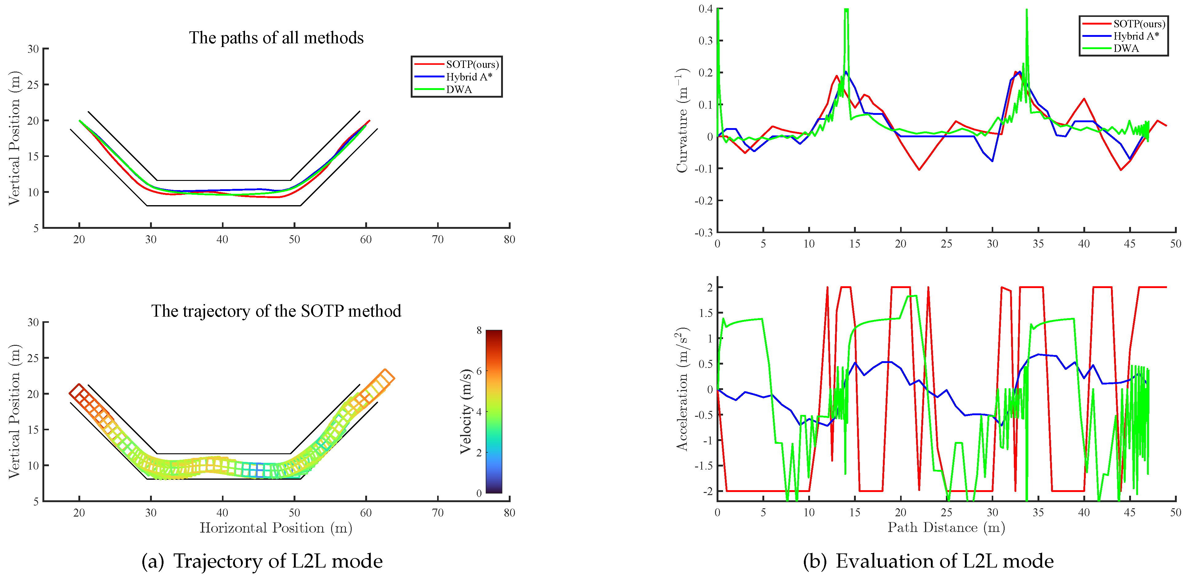
4.2.4. Trajectory Generation Result

We draw the generated trajectories and the evaluation results of all methods in Figure 9 for the L2L mode while in Figure 10 for the R2L mode. We know that vehicle operation in a narrow corridor is very hard, especially at the corridor corner, because of the requirement of more free area for turning. As shown in Figure 9a and Figure 10a, the trajectories planned by the SOTP method in both the L2L mode and R2L mode approach the outer boundaries before turning while to the inner boundaries in the other areas. This phenomenon conforms to the fact that the vehicle with the proposed method can find more free space before turning compared with other baseline methods and it needs to shorten the trajectory to save travel time in the other areas. Additionally, as the velocity heat distribution shown in Figure 9a and Figure 10a, the planned velocity would slow down before and rise up after turning, which is in accordance with the characteristics of actual vehicle rides. Therefore, the trajectories generated by the SOTP method in both corridors with the L2L and R2L modes are qualitatively reasonable.
The evaluation results including the curvature and the acceleration are shown in Figure 9b and Figure 10b. More details concerning the maximum curvature, maximum acceleration, and average velocity are recorded in Table 3. From Figure 9b and Figure 10b, the curvature of the DWA method changes sharply at each corner while the SOTP method and hybrid A* can availably restrain the curvature below 0.2 m 1 . As for the acceleration, both the SOTP method and the hybrid A* method can keep the acceleration in the allowable scope while the travel time of the SOTP method is shorter than the hybrid A* method. Furthermore, the computational time of the SOTP method is far less than that of the hybrid A* method which presents the proposed method has more powerful computational performance.
It is concluded that the proposed method has the highest computational efficiency and shortest travel time with the highest average velocity compared with other baseline methods while its acceleration and curvature could also satisfy the motion limitation.

4.3. Sensitivity Analysis

As designed in Equation (24), we use the fitted circles to approximate the vehicle shape for collision avoidance constraints. In this case study, we utilize different fitted circle numbers to generate trajectory while the other parameters are the same as the previous setting. The safety margin r is 1.24 m, 1.05 m, and 0.99 m with the case of N c = 3 , N c = 5 , and N c = 7 respectively. The planned trajectories are shown in the Figure 11 while the evaluation results are shown in the Table 4. With the fitted circle number increasing, the planned trajectory is smoother with a higher velocity in that the more fitted circles could reduce the redundant area, as a consequence of enlarging the feasible solution space. The trajectories with N c = 5 and N c = 7 have little difference indicating that the performance could not be improved by continuously increasing the fitted circles. The computational time of the L2L mode is totally greater than the R2L mode as a result of the limited space used to correct the vehicle posture for passing the next corner.

5. Field Experiment

Regarding the field test, we plan the trajectories by the SOTP method and the hybrid A* method separately and establish controller to track them in a real environment on a modified vehicle with an autopilot system.

5.1. Experiment Setup

In the field test, we test the trajectory planning and tracking in Narrow Corridor NC10, which is the most rigorous among the five narrow corridors introduced above. We ignore the generated velocity profiles and replace them with a constant speed of 10.8 km/h here for the safety concerns in real narrow corridor scenes. The vehicle parameters and the motion limitations are shown in Table A2 and Table A3 respectively.
The field test is conducted on a modified Lincoln MKZ platform as shown in Figure 12. The platform is equipped with an integrated Global Navigation Satellite System (GNSS) and an Inertial Measurement Unit (IMU). The vehicle also supports the by-wire control of the throttle, brake, steering and gear shifting system. The algorithms of motion planning and trajectory tracking control are implemented in C++ under Robot Operating System (ROS). Additionally, the parameters of the SOTP method and the hybrid A* method are the same as the previous setting. After generating the target trajectory, the vehicle is controlled by a nonlinear model predictive control algorithm introduced in [39] to track the planned trajectory at frequencies in excess of 100 Hz.

5.2. Experiment Result

The trajectories tracking results are shown in Figure 13, including the path tracking performance and the path tracking error. The lower tracking error shows that the trajectory could be tracked more easily and the corresponding method can be used in the real world more widely.
The vehicle planned paths and the corresponding tracking paths in the field test are shown in Figure 13a. Intuitively, the dotted red path almost completely overlaps with the solid red path, while the dotted blue path has an obvious gap with the solid blue line. An objective illustration of the path tracking result is shown in the Figure 13b. The centimeter-level tracking error here is related to both the advanced tracking control algorithm and the low testing speed for safety concerns. Anyway, the peak value in red is only 0.01 m while the peak value in blue is almost 0.045 m, which means the tracking error in red is much less than that in blue. Moreover, the fluctuation frequency of the tracking error in red is much gentler than that in blue. Hence, it can be concluded that the SOTP method is superior indeed.

6. Conclusions

This paper presents a space discretization-based optimal trajectory planning method for automated vehicles in narrow corridor-related scenes, which we name the SOTP method. With the space discretization strategy, we take the pre-discretized centerline waypoints as a reference and construct the optimal trajectory generation model totally in the space domain. An objective function in the trajectory optimization model is designed considering the travel time, with the goal of high efficiency. For constraints, vehicle kinematics, boundary collision avoidance, side force, actuator range limitation, terminal states, and boundary collision-free constraints are considered to make sure that the generated trajectory is safe and feasible. The proposed SOTP method is verified with both simulations and field experiments. The results show that the SOTP method is capable of generating feasible, smooth, and collision-free trajectories in narrow corridor scenarios. Furthermore, compared to the popular hybrid state A* algorithm, the SOTP method owns higher efficiency to generate a trajectory in the narrow corridor scene and the generated trajectories are smoother and more efficient. Moreover, the tracking performance of the trajectories planned by the SOTP method is much better, which would lead to more stable conditions for vehicle rides. Consequently, the proposed method has ability to plan a feasible trajectory in a narrow corridor scenario regarded as a corner case in the autonomous driving, potentially overcoming the limitation of other search-based methods.
We consider a static scenario with the predefined passable corridor which may depend on the high definition map. Therefore, in future works, we are going to consider the narrow corridor scenario with dynamic obstacles and uncertainty such as the sudden appearance of a pedestrian shielded by other obstacles to explore a more universal method.

Author Contributions

Conceptualization, B.X. and M.H.; methodology, B.X.; writing—original draft preparation, X.L. and S.Y.; formal analysis, M.H., Y.B. and Z.Q. All authors have read and agreed to the published version of the manuscript.

Funding

This research was funded by National Key R&D Program of China, grant number 2021YFB2501800, National Natural Science Foundation of China, grant number 52102394, 52172384, and 52222216, and Hunan Provincial Natural Science Foundation of China, grant number 2021JJ40095 and 2021JJ40065.

Data Availability Statement

Not applicable.

Acknowledgments

The authors sincerely thanks to associate professor Bai Li of Hunan University for his critical discussion and reading during manuscript preparation.

Conflicts of Interest

The authors declare no conflict of interest.

Appendix A

Table A1. Narrow corridor parameters.
SymbolMeaningValue
W L 2 L Corridor width (L2L)3.5 m
T1 L 2 L The first corridor turning angle (L2L) 135
T2 L 2 L The second corridor turning angle (L2L) 135
W R 2 L Corridor width (R2L)3.5 m
T1 R 2 L The first corridor turning angle (R2L) 135
T2 R 2 L The second corridor turning angle (R2L) 135
Table A2. Vehicle size parameters.
SymbolMeaningValue
lVehicle length4.925 m
LVehicle wheelbase2.850 m
l f Vehicle front overhang1.076 m
wVehicle width1.864 m
Table A3. Vehicle motion parameters.
SymbolMeaningValue
α max The maximum steering angle 30
ω max The limitation of wheel steering angular velocity 30 · s 1
v max The maximum allowable vehicle speed10 m · s 1
v min The minimum allowable vehicle speed1 m · s 1
a max The maximum limitation of vehicle acceleration2 m · s 2
a min The maximum limitation of vehicle deceleration−2 m · s 2
μ The adhesive coefficient0.3
gThe gravity coefficient9.8 m · s 2

References

  1. Milakis, D.; Arem, B.V.; Wee, B.V. Policy and society related implications of automated driving: A review of literature and directions for future research. J. Intell. Transp. Syst. 2017, 21, 324–348. [Google Scholar] [CrossRef]
  2. Chan, T.K.; Chin, C.S. Review of Autonomous Intelligent Vehicles for Urban Driving and Parking. Electronics 2021, 10, 1021. [Google Scholar] [CrossRef]
  3. Guo, Z.; Huang, Y.; Hu, X.; Wei, H.; Zhao, B. A Survey on Deep Learning Based Approaches for Scene Understanding in Autonomous Driving. Electronics 2021, 10, 471. [Google Scholar] [CrossRef]
  4. Li, B.; Tang, S.; Zhang, Y.; Zhong, X. Occlusion-Aware Path Planning to Promote Infrared Positioning Accuracy for Autonomous Driving in a Warehouse. Electronics 2021, 10, 3093. [Google Scholar] [CrossRef]
  5. Ziegler, J.; Bender, P.; Schreiber, M.; Lategahn, H.; Strauss, T.; Stiller, C.; Dang, T.; Franke, U.; Appenrodt, N.; Keller, C.G.; et al. Making bertha drive—an autonomous journey on a historic route. IEEE Intell. Transp. Syst. Mag. 2014, 6, 8–20. Available online: https://ieeexplore.ieee.org/document/6803933 (accessed on 15 November 2022). [CrossRef]
  6. Vu, T.M.; Moezzi, R.; Cyrus, J.; Hlava, J. Model Predictive Control for Autonomous Driving Vehicles. Electronics 2021, 10, 2593. [Google Scholar] [CrossRef]
  7. Sharma, O.; Sahoo, N.C.; Puhan, N.B. Recent advances in motion and behavior planning techniques for software architecture of autonomous vehicles: A state-of-the-art survey. Eng. Appl. Artif. Intell. 2021, 101, 104211. [Google Scholar] [CrossRef]
  8. Paden, B.; Čáp, M.; Yong, S.Z.; Yershov, D.; Frazzoli, E. A survey of motion planning and control techniques for self-driving urban vehicles. IEEE Trans. Intell. Veh. 2016, 1, 33–55. Available online: https://ieeexplore.ieee.org/document/7490340 (accessed on 15 November 2022). [CrossRef] [Green Version]
  9. Zhang, C.; Chu, D.; Liu, S.; Deng, Z.; Wu, C.; Su, X. Trajectory planning and tracking for autonomous vehicle based on state lattice and model predictive control. IEEE Intell. Transp. Syst. Mag. 2019, 11, 29–40. Available online: https://ieeexplore.ieee.org/abstract/document/8668708 (accessed on 15 November 2022). [CrossRef]
  10. Jiang, B.; Li, X.; Zeng, Y.; Liu, D. Human-Machine Cooperative Trajectory Planning for Semi-Autonomous Driving Based on the Understanding of Behavioral Semantics. Electronics 2021, 10, 946. [Google Scholar] [CrossRef]
  11. Li, B.; Ouyang, Y.; Li, L.; Zhang, Y. Autonomous Driving on Curvy Roads Without Reliance on Frenet Frame: A Cartesian-Based Trajectory Planning Method. IEEE Trans. Intell. Transp. Syst. 2022, 23, 15729–15741. [Google Scholar] [CrossRef]
  12. González, D.; Pérez, J.; Milanés, V.; Nashashibi, F. A review of motion planning techniques for automated vehicles. IEEE Intell. Trans. Intell. Transp. Syst. 2015, 17, 1135–1145. Available online: https://ieeexplore.ieee.org/document/7339478 (accessed on 15 November 2022). [CrossRef]
  13. Fraichard, T.; Scheuer, A. From Reeds and Shepp’s to continuous-curvature paths. IEEE Trans. Robot. 2004, 20, 1025–1035. Available online: https://ieeexplore.ieee.org/document/1362698 (accessed on 15 November 2022). [CrossRef] [Green Version]
  14. Bae, I.; Kim, J.H.; Moon, J.; Kim, S. Lane Change Maneuver based on Bezier Curve providing Comfort Experience for Autonomous Vehicle Users. In Proceedings of the 2019 IEEE Intelligent Transportation Systems Conference (ITSC), Auckland, New Zealand, 27–30 October 2019; pp. 2272–2277. [Google Scholar]
  15. Elbanhawi, M.; Simic, M. Sampling-based robot motion planning: A review. IEEE Access 2014, 2, 56–77. Available online: https://ieeexplore.ieee.org/abstract/document/6722915/ (accessed on 15 November 2022). [CrossRef]
  16. Zheng, K.; Liu, S. RRT based path planning for autonomous parking of vehicle. In Proceedings of the 2018 IEEE 7th Data Driven Control and Learning Systems Conference (DDCLS), Enshi, China, 25–27 May 2018; pp. 627–632. [Google Scholar]
  17. Stentz, A. Optimal and efficient path planning for partially known environments. In Proceedings of the 1994 IEEE International Conference on Robotics and Automation (ICRA), San Diego, CA, USA, 8–13 May 1994; pp. 3310–3317. [Google Scholar]
  18. Min, H.; Xiong, X.; Wang, P.; Yu, Y. Autonomous driving path planning algorithm based on improved A* algorithm in unstructured environment. Proc. Inst. Mech. Eng. Part D J. Automob. Eng. 2021, 235, 513–526. [Google Scholar] [CrossRef]
  19. Li, C.; Du, J.; Liu, B.; Li, J. A Path Planning Method Based on Hybrid A-Star and RS Algorithm. In Proceedings of the 3rd International Forum on Connected Automated Vehicle Highway System, Jinan, China, 23–25 October 2020. [Google Scholar]
  20. Dirik, M.; Kocamaz, F. RRT-Dijkstra: An Improved Path Planning Algorithm for Mobile Robots. J. Soft Comput. Artif. Intell. 2020, 1, 69–77. Available online: https://dergipark.org.tr/en/pub/jscai/issue/56697/784679 (accessed on 15 November 2022).
  21. Kogan, D.; Murray, R. Optimization-based navigation for the DARPA Grand Challenge. In Proceedings of the 45th IEEE Conference on Decision and Control (CDC), San Diego, CA, USA, 13–15 December 2006. [Google Scholar]
  22. Li, S.; Li, Z.; Yu, Z.; Zhang, B.; Zhang, N. Dynamic trajectory planning and tracking for autonomous vehicle with obstacle avoidance based on model predictive control. IEEE Access 2019, 7, 132074–132086. Available online: https://ieeexplore.ieee.org/document/8835033/ (accessed on 15 November 2022). [CrossRef]
  23. Dixit, S.; Montanaro, U.; Dianati, M.; Oxtoby, D.; Mizutani, T.; Mouzakitis, A.; Fallah, S. Trajectory planning for autonomous high-speed overtaking in structured environments using robust MPC. IEEE Intell. Trans. Intell. Transp. Syst. 2019, 21, 2310–2323. Available online: https://ieeexplore.ieee.org/document/8734145 (accessed on 15 November 2022). [CrossRef]
  24. Zhu, S.; Aksun-Guvenc, B. Trajectory Planning of Autonomous Vehicles Based on Parameterized Control Optimization in Dynamic on-Road Environments. J. Intell. Robot. Syst. 2020, 100, 1055–1067. Available online: https://link.springer.com/article/10.1007/s10846-020-01215-y (accessed on 15 November 2022). [CrossRef]
  25. Szkandera, J.; Kolingerová, I.; Maňák, M. Narrow passage problem solution for motion planning. In Proceedings of the International Conference on Computational Science (ICCS), Amsterdam, The Netherlands, 3–5 June 2020; pp. 459–470. [Google Scholar]
  26. Kim, D.; Chung, W.; Park, S. Practical motion planning for car-parking control in narrow environment. IET Control. Theory Appl. 2010, 4, 129–139. [Google Scholar] [CrossRef]
  27. Li, B.; Yin, Z.; Ouyang, Y.; Zhang, Y.; Zhong, X.; Tang, S. Online Trajectory Replanning for Sudden Environmental Changes During Automated Parking: A Parallel Stitching Method. IEEE Trans. Intell. Veh. 2022, 7, 748–757. [Google Scholar] [CrossRef]
  28. Do, Q.H.; Mita, S.; Yoneda, K. Narrow passage path planning using fast marching method and support vector machine. In Proceedings of the 2014 IEEE Intelligent Vehicles Symposium Proceedings (IV), Ypsilanti, CA, USA, 8–11 June 2014; pp. 630–635. [Google Scholar]
  29. Tian, X.; Fu, M.; Yang, Y.; Wang, M.; Liu, D. Local Smooth Path Planning for Turning Around in Narrow Environment. In Proceedings of the 28th IEEE International Symposium on Industrial Electronics (ISIE), Vancouver, BC, Canada, 12–14 June 2019; pp. 1924–1929. [Google Scholar]
  30. Li, B.; Acarman, T.; Zhang, Y.; Zhang, L.; Yaman, C.; Kong, Q. Tractor-trailer vehicle trajectory planning in narrow environments with a progressively constrained optimal control approach. IEEE Trans. Intell. Veh. 2020, 5, 414–425. [Google Scholar] [CrossRef]
  31. Li, B.; Acarman, T.; Zhang, Y.; Ouyang, Y.; Yaman, C.; Kong, Q.; Zhong, X.; Peng, X. Optimization-Based Trajectory Planning for Autonomous Parking With Irregularly Placed Obstacles: A Lightweight Iterative Framework. IEEE Trans. Intell. Transp. Syst. 2022, 23, 11970–11981. [Google Scholar] [CrossRef]
  32. Lin, X.; Xie, H.; Xu, B.; Yuan, S.; Bian, Y.; Hu, M.; Qin, Z.; Hu, J. A Vehicle Trajectory Planning Method for Narrow Corridor in Mines Based on Optimal Control. Control Inf. Technol. 2022, 05, 23–29. Available online: https://kns.cnki.net/kcms/detail/detail.aspx?filename=BLJS202205004&dbname=cjfdtotal&dbcode=CJFD&v=MTE0NzhSNkRnOC96aFlVN3pzT1QzaVFyUmN6RnJDVVI3aWVaZWRyRmkza1Y3N0JKeUhCZmJHNEhOUE1xbzlGWUk= (accessed on 15 November 2022).
  33. Rajamani, R. Vehicle Dynamics and Control, 2nd ed.; Springer: New York, NY, USA, 2012; pp. 24–25. [Google Scholar]
  34. Ziegler, J.; Bender, P.; Dang, T.; Stiller, C. Trajectory planning for Bertha—A local, continuous method. In Proceedings of the 2014 IEEE Intelligent Vehicles Symposium Proceedings (IV), Ypsilanti, CA, USA, 8–11 June 2014; pp. 450–457. [Google Scholar]
  35. Biegler, L.T.; Zavala, V.M. Large-scale nonlinear programming using IPOPT: An integrating framework for enterprise-wide dynamic optimization. Comput. Chem. Eng. 2009, 33, 575–582. [Google Scholar] [CrossRef]
  36. Thrun, S.; Montemerlo, M.; Dahlkamp, H.; Stavens, D.; Aron, A.; Diebel, J.; Mahoney, P. Stanley: The robot that won the DARPA Grand Challenge. J. Field Robot. 2006, 23, 661–692. [Google Scholar] [CrossRef]
  37. Fox, D.; Burgard, W.; Thrun, S. The dynamic window approach to collision avoidance. IEEE Robot Autom. Mag. 1997, 4, 23–33. [Google Scholar] [CrossRef]
  38. Dolgov, D.; Thrun, S.; Montemerlo, M.; Diebel, J. Practical search techniques in path planning for autonomous driving. In Proceedings of the First International Symposium on Search Techniques in Artificial Intelligence and Robotics (STAIR-08), Chicago, IL, USA, 13–14 July 2008. [Google Scholar]
  39. Yin, C.; Xu, B.; Chen, X.; Qin, Z.; Bian, Y.; Sun, N. Nonlinear Model Predictive Control for Path Tracking Using Discrete Previewed Points. In Proceedings of the 2020 IEEE 23rd International Conference on Intelligent Transportation Systems (ITSC), Rhodes, Greece, 20–23 September 2020; pp. 1–6. [Google Scholar]
Figure 1. A typical narrow corridor with definite boundaries. The corridor is comprised of three segments. Hence, this corridor can be represented by the parameter groups A i l , B i l , C i l and A i r , B i r , C i r , i { 1 , 2 , 3 } .
Electronics 11 04239 g001
Figure 2. The kinematic model with front-wheel steering.
Electronics 11 04239 g002
Figure 3. Corridor division. The turning area at the corridor is determined by the fixed road turning center and corridor turning angle.
Electronics 11 04239 g003
Figure 4. Centerline discretization. The upper formula represents the left boundary while the lower formula represents the right boundary.
Electronics 11 04239 g004
Figure 5. Diagram of the circle fitting strategy.
Electronics 11 04239 g005
Figure 6. Corridor boundary-collision checking in trajectory planning.
Electronics 11 04239 g006
Figure 7. The simulation results in the single corner scenario. (a) the trajectory planning result and (b) the trajectory tracking result. The minimum turning angle of the proposed method is 120 and the trajectory could be tracked in different corner angles.
Electronics 11 04239 g007
Figure 8. Typical continuous turning situations in narrow corridors with (a) presents the L2L mode and (b) presents the R2L mode.
Electronics 11 04239 g008
Figure 9. Trajectory generated by all methods in the narrow corridor scene with heat distribution indicating the velocity change. (a) the trajectory planned in the L2L mode. (b) the curvature and acceleration profile of the trajectories in the L2L mode.
Electronics 11 04239 g009
Figure 10. Trajectory generated by all methods in the narrow corridor scene with heat distribution indicating the velocity change. (a) the trajectory planned in the R2L mode. (b) the curvature and acceleration profile of the trajectories in the R2L mode.
Electronics 11 04239 g010
Figure 11. Trajectory generated by the SOTP method with different fitted circle numbers in the narrow corridor scene with the velocity curve. (a) the trajectory planned in the L2L mode. (b) the trajectory planned in the R2L mode.
Electronics 11 04239 g011
Figure 12. The modified Lincoln MKZ with an autopilot system used in the field experiment.
Electronics 11 04239 g012
Figure 13. The trajectories tracking results in the field experiment. (a) the path tracking performance (b) the path tracking error.
Electronics 11 04239 g013
Table 1. Narrow corridor cluster parameters.
SymbolMeaningValue
NC1Corner angle of the first narrow corridor180
NC2Corner angle of the second narrow corridor175
NCzCorner angle of the z th narrow corridor(185-5z)
W NC Corridor width of the narrow corridors3.5 m
Table 2. The proposed method parameters.
SymbolMeaningValue
Δ x The allowable error in the x-axis0.0625 m
Δ y The allowable error in the y-axis0.0625 m
Δ θ The allowable heading error0.0685 rad
N c The number of fitted circles3
NThe number of discrete waypoints60
Table 3. The evaluation results.
MethodModeMax. Curvature (m 1 )Max. Acceleration (m/s 2 )Avg. Velocity (m/s)Travel Time (s)Computational Time (s)
Hybrid A starL2L0.200.703.9612.2183.83
R2L0.180.834.3310.9177.35
DWAL2L0.692.331.7727.6848.65
R2L0.622.421.4733.3382.62
SOTP(ours)L2L0.202.004.3911.1630.91
R2L0.202.004.8410.119.37
Table 4. The result of sensitivity analysis.
Fitted Circle NumberModeMax. Curvature (m 1 )Max. Acceleration (m/s 2 )Avg. Velocity (m/s)Travel Time (s)Computational Time (s)
N c = 3 L2L0.202.004.3911.1630.91
R2L0.202.004.8410.119.37
N c = 5 L2L0.132.006.757.2729.29
R2L0.122.006.837.175.62
N c = 7 L2L0.122.006.947.0533.03
R2L0.112.006.977.018.21
Publisher’s Note: MDPI stays neutral with regard to jurisdictional claims in published maps and institutional affiliations.

