Intelligent Fault Diagnosis Method for Industrial Processing Equipment by ICECNN-1D

Abstract

Intelligent algorithm has been widely implemented to effectively diagnose faults in industrial instrument, electrical equipment and mechanical equipment. In addition, the rapid development of sensing technology generated enormous time series signal. Accordingly, diagnosing faults by analyzing time series signal has been widely developed. This paper aims to diagnose faults by applying improved Convolution Neural Network with Compression Enhancement (ICECNN-1D) to analyze time series signal, which effectively considers time series property of signal while diagnosing faults by artificial intelligence. Additionally, a large number of trend features and fluctuation features in high-frequency time series are also considered. the recognition rates of almost other machine learning algorithm are less than 90% in the experiments. Other methods may provide high rate of recognition, but their fluctuation of the recognition rate has varied obviously with different loads, and results provide undesirable ability of generalization under different working conditions. Comparatively, ICECNN-1D model provides high recognition rate and terrific ability of generation while processing time series with high frequency, and its accuracy of the recognition rate fluctuates inconspicuously with different loads.

1. Introduction

Failures in electrical equipment, industrial instruments and mechanical equipment are some of the main factors that lead to abnormal industrial processes [1]. Consequently, to solve such problems, methods to diagnose faults in industrial processes have been investigated in recent decades. Moreover, many scholars have, in particular, tried to diagnose faults in power systems. Methods of detecting and diagnosing faults in traction systems have been introduced [2]. Moreover, weighted Sliding Hilbert Transform (WSHT) has been applied to estimate instantaneous amplitude to diagnose faults in power systems in wind turbines [3]. Finally, faults in power switches’ open-circuits and current sensors faults have been diagnosed using Sliding Mode Observer [4].

Recently, machine learning has been widely implemented to detect and diagnose faults. First of all, a cost function which apllied several clusters in machine learning algorithm with optimal sensor placement was introduced to diagnose faults in mechanical equipment. Therefore, a machine learning algorithm that optimizes model parameters in the diagnosis system was designed [5]. Secondly, a scheme to classify bearing faults based on Support Vector Machine was evaluated by analyzing vibration data of bearings under different work conditions [6]. Additionally, a machine learning algorithm with optimized parameters was implemented to generate simulated vibration signals during actual shock and mixed failures; it aims to identify the faulty gearbox under various speeds [7]. In addition, machine learning and natural language processing methods were implemented to diagnose faults in railway signaling equipment, which can reduce the technical requirements for on-site maintenance personnel [8]. Finally, a focused literature survey of machine learning and data mining methods for fault diagnosis and methodological research in support of smart devices was introduced [9].

In recent decades, the increasing scale of data size has augmented the difficulty of using machine learning to diagnose faults [10,11]. Consequently, the application of deep learning to diagnose faults in manufacturing equipment has become a novel method. Initially, deep-SincNet, a deep learning architecture which is applied for Multi-Fault Diagnosis Tasks, was proposed to learn fault features from raw motor currents [12]. Furthermore, a Single-Side Canonical Correlation Analysis fault detection framework with the aid of a Neural Network to detect faults in industrial equipment was introduced [13]. Furthermore, an intelligent method to reduce the complexity of a training model by mining data was proposed. This method applied a Bayesian network to deduce fault symptoms from historical fault data [14]. Lastly, in order to solve problems in hydraulic systems, such as difficulty in acquiring parameters and a system containing many faults, uncertainty and concealment, various hydraulic system fault diagnosis techniques and methods were analyzed [15].

In recent years, with the development of deep learning, various novel CNN-1D networks have been used in the field of fault diagnosis and have achieved good diagnosis results [16,17,18,19,20]. However, it is still difficult to extract the high-frequency fault features of micro faults, which affects the early fault diagnosis of industrial process equipment.

This paper introduced a method to diagnose fault by applying improved Convention Neural Network with Compression Enhancement (ICECNN-1D) to analyze time-series signal. Contributions of this paper can be summarized as follows:

(1) To solve the problem that the use of intelligent algorithms to diagnose faults has not involved the consideration of time series properties of signals, a fault diagnosis method based on an audio–visual fusion algorithm was proposed. As a result, machine learning algorithms effectively utilized information about time series while diagnosing faults.

(2) In conventional CNN-1D, time series need to be divided into time series with a certain width as its input, which will cause the loss of the deep features of time series signals changing with time during the training and learning process. Although CECNN-1D can effectively extract high-frequency fault features through compression enhancement, the correlation between high-frequency features and faults is weakened. Therefore, the global pooling layer is used in the ICECNN-1D model instead of the full connection layer in the CECNN-1D model, which makes full use of a large number of signal trend features and fluctuation features hidden in the high-frequency time series for fault detection, which makes the model more stable.

2. Fault Diagnosis Method Based on ICECNNN-1D

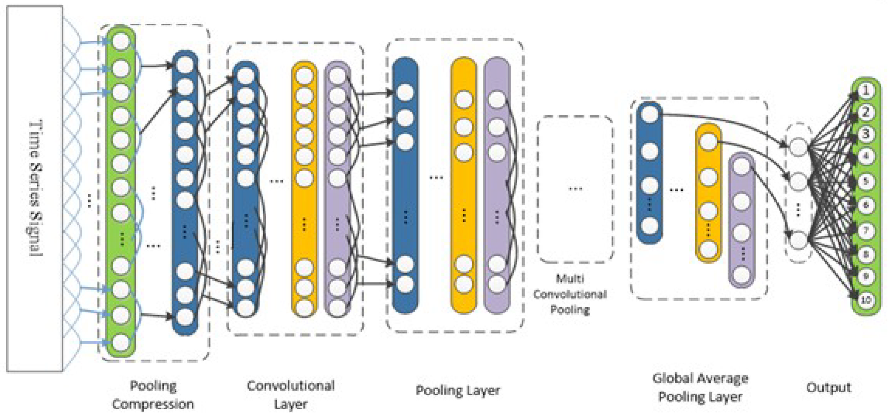
2.1. Basic Concept of Convolutional Neural Network with Compression Enhancement

Conventional Neural Networks (CNNs) are composed of a convolutional layer, a down sampling layer, an activation function and a connected layer [21,22]. The convolutional layer is made of several convolutional kernels which divide images into small parts to help to extract features. Secondly, the down-sampling layer was adopted to reduce the dimensionality of the kernel, which aims to decrease computation and increase the receptive field. Thirdly, the activation function was located at the end of the Neural Network model to increase the speed of the learning process [22]. In addition, one-dimensional CNN (1D-CNN) regarded the convolutional kernel as a window. Then, the time series signal needs to translate following this window to acquire local information and extract local features from dot product results from features and weights. To solve the problem that a traditional CNN does not consider the time series character of one-dimensional time series signals, to effectively extract features of time series signals with high frequency, the ICECNN-1D Neural Network model, which is shown in Figure 1, was proposed.

CECNN-1D is different from traditional Neural Networks. The proposed method added a two-level pooling compression layer to compress and reduce time series signals. The first layer extracts the average signal features of each segment and the second layer uses the maximum pooling to extract important feature information. A large amount of redundant information in time series signals with high frequencies is removed by using two-layer cascade pooling. The audio–visual information of a one-dimensional signal can be effectively fused by using two-layer cascading pooling. Moreover, a large amount of redundant information from time series signals with high-frequency can be removed so that features are effectively extracted from high-frequency signals by subsequent operations. On the other hand, according to Figure 1, the proposed method ICECNN-1D replaces the full connection layer in CECNN-1D with a global average pooling layer after multiple convolution and pooling layers. The global average pooling layer can get a corresponding output for each feature graph by averaging each output feature graph. This layer does not need training parameters. Compared with the full connection layer, it can significantly reduce the number of model parameters and improve the training speed. At the same time, it can enhance the correlation between features and target categories, enhance the nonlinear expression ability of the model, and finally transfer its features to the Softmax layer for multi fault feature classification.

2.2. Audio–Visual Information Fusion Methods Based on One-Dimensional Signal

When mechanical equipment fails, the detected signal of sensors has changed accordingly. Therefore, extracting and analyzing different fault features become an important part of fault diagnosis, especially in intelligent fault diagnosis systems based on signal processing and knowledge. The method to analyze signals is an important prerequisite of diagnosis accuracy.

One-dimensional signal features and two-dimensional image features have a corresponding relationship, so images are represented by color histograms. Consequently, one-dimensional signals can be extracted by layering. Therefore, the theoretical basis of the audio–visual fusion method in this study is constructed.

(1) Correspondence between image features and one-dimensional signal features.

The two-dimensional image is expanded by rows and columns to form a single signal $x_i$, where $i=1,2,3,\dots ,N$, if discarding the spatial characteristics of the image. The image mean is defined as:

$$\overline{x}=\frac{1}{n}\sum _{k=1}^n{x}_i$$

(1)

Accordingly, the standard deviation is defined as:

$$s=\sqrt{\frac{1}{n-1}\sum _{k=1}^n{(xi-\overline{x})}^2}$$

(2)

Moreover, the covariance function is defined as:

$$cov(x,y)=E\left[\right(x-\mu \left)\right(y-\eta \left)\right]$$

(3)

The function of the correlation coefficient is defined as:

$$S(i,j)=\frac{C(i,j)}{\sqrt{C(i,i)C(j,j)}}$$

(4)

The autocorrelation function of the image is defined as:

$$C(\epsilon ,\eta ,j,k)=\frac{s{\sum }_{m=j-w}^{j+w}{\sum }_{m=k-w}^{k+w}f(m,n)f(m-\epsilon ,n-\eta )}{\sum m_{m=j-w}^{j+w}{\sum }_{n=k-w}^{k+w}{\left[f(m,n)\right]}^2}$$

(5)

Experiments show that the texture of the image is related to its original position and the magnitude of the energy. As a result, if the arrangement of energy is concentrated and it is close to the original position, the texture of the image is thicker. Conversely, if the energy’s arrangement is dispersed and it is farther from original position, the texture of the image is thinner [23].

The normalized co-occurrence matrix S in the gray-level co-occurrence matrix $V_{\lambda }(p,q)$ is applied to describe the probability distribution of pixel pairs at a certain spatial position:

$$W_{\lambda }=\frac{V_{\lambda }(p,q)}{S}$$

(6)

Then the feature of color’s second layer in the signal is $f_1$, which describes the uniformity of the grayscale distribution of the image. A coarse texture image means a larger value of $f_1$ and more energy consumption. Conversely, a fine texture image means a smaller value of $f_1$ and less energy consumption.

$$f_1=\sum _{i=0}^{L-1}\sum _{j=0}^{L-1}{W}_{\lambda }^2(p,q)$$

(7)

Simultaneously, $f_2$ describes the sharpness of image texture.The clearer texture means larger $f_2$ value.

$$f_2=\sum _{n=0}^{L-1}{n}^2\left\{\sum _{i=0}^{L-1}\sum _{j=0}^{L-1}{W}_{\lambda }^2(p,q)\right\}$$

(8)

where

$$n=\left|i-j\right|$$

(9)

The entropy value is $f_3$, which describes the amount of information in the image texture. A more textured image indicates a larger $f_3$ value.

$$f_3=-\sum _{i=0}^{L-1}\sum _{j=0}^{L-1}{W}_{\lambda }(p,q)log\left. [W_{\lambda }(p,q)\right]$$

(10)

Assuming that the discrete signal sequence is $\left\{x_i\right\}$ where $i=1,2,3,\dots ,N$, the above six characteristic parameters are defined as follows:

$$S={}^{{{\displaystyle \sum _{i=1}^N}(xi-\overline{x})}^3}/{}_{(N-1){\sigma }^3}$$

(11)

Simultaneously, the kurtosis Equation is:

$$K={\sum _{i=1}^N(x_i-\overline{x})}^3/(N-1){\sigma }^4$$

(12)

Therefore, the peak indicators (CF) are calculated by:

$$CF=max\left|x_i\right|/\sqrt{\frac{1}{N}\sum _{i=1}^N{\left(x_i\right)}^2}$$

(13)

The pulse index (IF) is:

$$IF=max\left|x_i\right|/\frac{1}{N}\sum _{i=1}^N\left|x_i\right|$$

(14)

The waveform indicators (SF) are:

$$SF={}^{\sqrt{N{\displaystyle \sum _{i=1}^N}{\left(x_i\right)}^2}}/{}_{{\displaystyle \sum _{i=1}^N}\left|x_i\right|}$$

(15)

The measured state signals usually show a normal distribution if equipment is running normally, which indicates that state parameters of equipment are basically in the normal range [24]. Slopes S and K are used to indicate the degree to which the signal deviates from the normal distribution, so they are often implemented to characterize the occurrence of disturbances; the CF peak indicator is sensitive to weak signals that vary over time. Moreover, analyzing monitoring and CF peak indicator can help to predict early equipment failures. SF waveform indicator is more sensitive to pitting faults in rotating devices such as bearings; the intermediate frequency pulse index and the CLF range index are more sensitive to instantaneous failures, especially in the early stage of failure. However, if intermediate frequency pulse index and the CLF range index increase to a certain level, Results show a downward trend in the gradual development of faults, which indicates that the intermediate frequency pulse index and the CLF range index are highly sensitive to initial faults, but results are not stable.

(2) Color histogram of one-dimensional signal.

The color histogram has obvious differences if color changes. In order to describe fault characteristics, using color characteristics of the image, the statistical histogram can be established by implementing color features from the image. The parametric Equation (1) for the statistical histogram is:

$$H\left(k\right)=\frac{n_k}{N}k=0,1,\dots ,L-1$$

(16)

where $H\left(k\right)$ represents the kth histogram, N denotes the total number of data and $N_k$ is the number of data in the kth histogram. Then, the function to count the cumulative histogram of the image color feature is defined by:

$$I\left(k\right)=\sum _{i=0}^k\frac{n_i}{N}k=0,1,\dots ,L-1$$

(17)

where $I\left(k\right)$ represents the cumulative histogram within the time range k and $n_i$ is the number of data at time i. Additionally, $P_{ij}$ means the jth column of the ith row in the data P. Then, the function at the first layer of color is expressed as:

$$u_i=\frac{1}{N}\sum _{j=1}^n{P}_{ij}$$

(18)

This function is the average value of a segment of a signal, which is the average signal feature of a segment of a signal obtained by the first level pooling layer compression from the proposed ICECNN-1D network. Secondly, the function at the second layer of color is calculated by:

$${\sigma }_i={\left(\frac{1}{N}\sum _{j=1}^N{\left(P_{ij}-u_i\right)}^2\right)}^{\frac{1}{2}}$$

(19)

In addition, the function at the third layer of color is expressed as:

$$S_i={\left(\frac{1}{N}\sum _{j=1}^N{\left(P_{ij}-u_i\right)}^3\right)}^{\frac{1}{3}}$$

(20)

where $P_{ij}-u_i$ is the difference between the error of each column from data and the first function of the corresponding color. In this way, three-layer color function is similar to the three colors of an image, so it can use the same method as the image to construct a color histogram and extract local features. On the other hand, by associating the signal with the visual features, the second level maximum pooling layer global average pooling layer of ICECNN-1D network can be applied to compress and extract the important features of signal while removing redundant information.

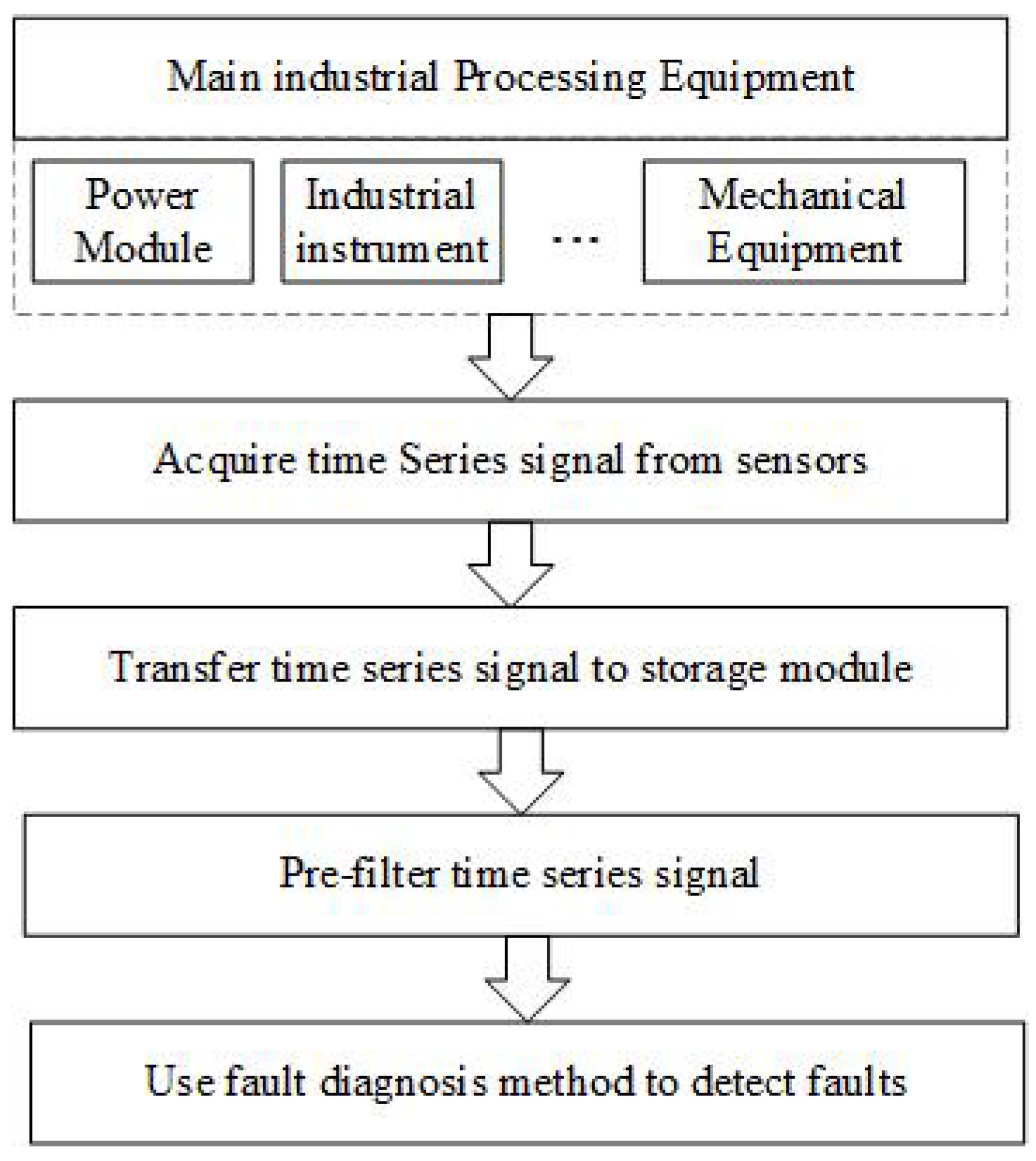
2.3. Working Principle Equipment Fault Diagnosis System

The general fault diagnosis service platform is an embodiment of “universal”, which means software settings that can be matched for any acquisition module. For the service platform introduced in this paper, the main point is versatility of the software platform. The service platform also contains several hardware acquisition modules, which are hardware acquisition modules verified by the system in this design. First of all, for most of the acquisition modules (including the hardware used in this system test), the schematic diagram is shown in Figure 2.

Figure 2 describes the whole process of diagnosing faults by introducing a mechanical fault diagnosis system which is composed of the following parts: First of all, a time series signal was acquired from different sensors such as an accelerometer and it was sent to the storage module from the computer. Then, the software part adopted the desktop application software based on JavaFX by using JDK1.8. The software provided basic functional modules such as real-time monitoring, data analysis (FFT, power spectrum, original signal, envelope spectrum, cepstrum), data management (historical data storage, real-time storage data, sampling data storage), system configuration, etc. Then, the vibration data were sampled and stored and the processing data were analyzed, thereby judging change in the vibration condition of the detected position, and slow change in the vibration effective value, peak value and frequency spectrum was shown through long-term data recording [25,26].

3. Intelligent Equipment Fault Diagnosis Experimental Scheme

This section presents experiments conducted to verify the performance of the ICECNN-1D model by using rotor bearing fault data from Case Western Reserve Bearing Data Center Website [27]. The vibration signal of the bearing with different failures was sampled with 48 kHz sample frequency. Motor bearings were seeded with faults using electro-discharge machining (EDM). Faults ranging from 0.007 inches in diameter to 0.040 inches in diameter were introduced separately at the inner raceway, rolling element (i.e., ball) and outer raceway. Faulted bearings were reinstalled into the test motor and vibration data were recorded for motor loads of 0 to 3 horsepower (motor speeds of 1797 to 1720 RPM). Vibration data were collected by using accelerometers, which were attached to the housing with magnetic bases. Accelerometers were placed at the 12 o’clock position at both the drive end and fan on end of the motor housing. During some experiments, an accelerometer was attached to the motor supporting the base plate as well. Vibration signals were collected by implementing a 16 channel DAT recorder. Additionally, digital data were collected at 12,000 samples per second and data were also collected at 48,000 samples per second for drive end bearing faults. Speed and horsepower data were collected using the torque transducer/encoder and were recorded manually. As shown in Figure 3, the bearing pitting fault diameter is 0.014 mm and the rotor bearing drive end inner race fault status data under different motor loads (motor speeds) whose values are 1797 rpm, 1772 rpm, 1750 rpm and 1730 rpm respectively.

Four datasets—A, B, C and D—were adopted in the experiments. A, B and C were datasets under motor loads of 1 hp, 2 hp and 3 hp (corresponding to motor speed of 1772 rpm, 1750 rpm and 1730 rpm, respectively). Each dataset includes 6650 training samples and 200 test samples. As a result, the training samples adopt dataset enhancement technology and there is no overlap phenomenon between test samples. Dataset D is the union of datasets A, B and C, which means it includes three load states, with a total of 19850 training samples and 700 test samples. The experimental datasets are described in

Table 1. Description of experimental datasets.

Fault Location		No	Rolling Element			Inner Raceway			Outer Raceway			Load
Label		1	2	3	4	5	6	7	8	9	10
Fault diameter (inch)		0	0.007	0.014	0.021	0.007	0.014	0.021	0.007	0.014	0.021
A	training	665	665	665	665	665	665	665	665	665	665	1
	Testing	20	20	20	20	20	20	20	20	20	20
B	training	665	665	665	665	665	665	665	665	665	665	2
	Testing	20	20	20	20	20	20	20	20	20	20
C	training	665	665	665	665	665	665	665	665	665	665	3
	Testing	20	20	20	20	20	20	20	20	20	20
D	training	1985	1985	1985	1985	1985	1985	1985	1985	1985	1985	1,2,3
	Testing	70	70	70	70	70	70	70	70	70	70

.

Five experiments were implemented to verify fault diagnosis performance of the introduced model by using time series signals with high frequency by comparing with the current mainstream model, The experiment was built by utilizing the TensorFlow framework and the specific training environment configuration is shown in

Table 2. Experimental environment setting.

Experimental Environment	Hardware Configuration
Operating system	Windows 11
CPU	Intel(R) Xeon(R) Gold 5218R cpu @ 2.10 GHz
GPU	NVIDIA GeForce RTX 3080
Tensorflow	1.14
python	3.7

. Moreover, different convolution kernel size was applied to analyze the performance of the introduced Neural Network model. All experimental settings are as follows: Let the batch size be equal to 120, and initial learning rate of Adam optimizer is 0.0015. Moreover, the input width of the signal is 2048*2, and iterative training is performed for 30 rounds. Therefore, 10 experiments are performed to obtain the average value.

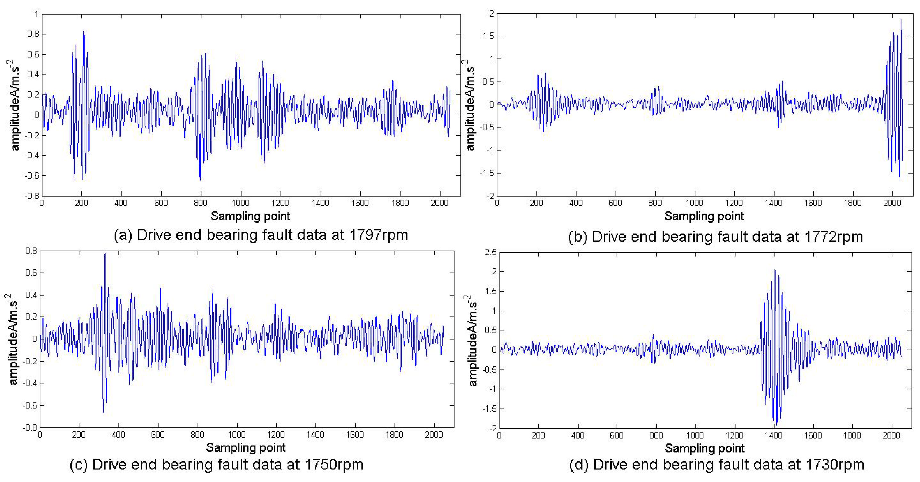
3.1. Experiment 1: Fault Diagnosis Effect of ICECNN-1D of High Frequency Time Series Signal

The first experiment compared training time and accuracy of diagnosing faults by the introduced method withNCNN-1D and ECNN-1D to analyze performance of the introduced method. Results perceived time series data with high-frequency and the effect of fault diagnosis are analyzed. The cascade pooling layer was removed from CECNN-1D and ICECNN-1D, and the first layer used 4*1 small convolution kernel model which is NCNN-1D and ECNN-1D respectively, the two models was implemented to compare with performance by the introduced model. The experimental results are shown in

Table 3. Experimental comparison results of NCNN-1D and CECNN-1D.

Model	Average Accuracy (%)		Average Time (s)
	Train	Test	Train	Test
NCNN-1D	0.9645	0.9532	223	0.79
ECNN-1D	0.9744	0.9776	164	0.71
ICECNN-1D	0.9782	0.9794	158	0.68

.

According to Table 3 shows that after the cascade pooling layer is removed, the average recognition rate of ECNN-1D is higher than that of NCNN-1D, and the average time is lower than that of NCNN-1D, which shows that using the global average pooling layer instead of the whole concatenated layer can effectively improve the accuracy of the model and reduce parameter training.

Meanwhile, the trend of the iteration umber was recorded by analyzing accuracy rate and loss function value by implementing two models. Additionally, experimental results were shown in Figure 4 and Figure 5:

According to Figure 4, the proposed method can provide better performance to train time series signal than performance by NCNN-1D and ECNN-1D. The tested trend curve provides great volatility and it rise with slow speed. However, the final recognition rate is not high, and it cannot fit well with the training recognition rate curve. Thereby, the overall training result of the model is not ideal.

According to Figure 5, the fitting effect of trained and tested curves is not ideal. However, the trained loss function value curve is often in a high range at the end, but the tested objective function value curve is in a lower range at the end, and the proposed method can also provide better convergence speed than NCNN-1D and ECNN-1D. Consequently, the trend curves of ICECNN-1D model training and provides good performance and result is accurate.

Recognition by ICECNN-1D model is effective because the average accuracy is 97.88%, and it takes less time. According to results from experiment 1, ICECNN-1D model provides some advantages such as effectively compressing high-frequency time series data, removing redundant information and reducing the dimension of data, which enhance the perception ability of high-frequency time series data and strengthening correlation between high-frequency time series signals and fault categories, and have better fault identification ability [28,29].

3.2. Experiment 2: Performance under Different Compression Sizes

It is necessary to analyze the performance of ICECNN-1D cascaded pooling layers under different compression sizes. Experiment 2 was carried out with compression sizes of 1*1 (uncompressed), 2*1, 3*1, 4*1, 5*1, 6*1,7*1, 8*1, 9*1, and 10*1, respectively. Moreover, experiments were carried out under data set B, The experimental results are shown in Figure 6.

According to Figure 6, the increasing compression size of the ICECNN-ID cascaded pooling layer caused the increasing accuracy rate, whose maximum recognition rate is at 97.87% when the size is 4. Experiment indicated the cascaded pooling operation can be used. Moreover, effectively compress and filter high-frequency time series data can remove redundant information. High frequency information can also be effectively expressed through global average pooling and achieve a certain enhancement effect [30]. Therefore, the ICECNN-1D model adopted a small-sized compression length, which can increase recognition accuracy.

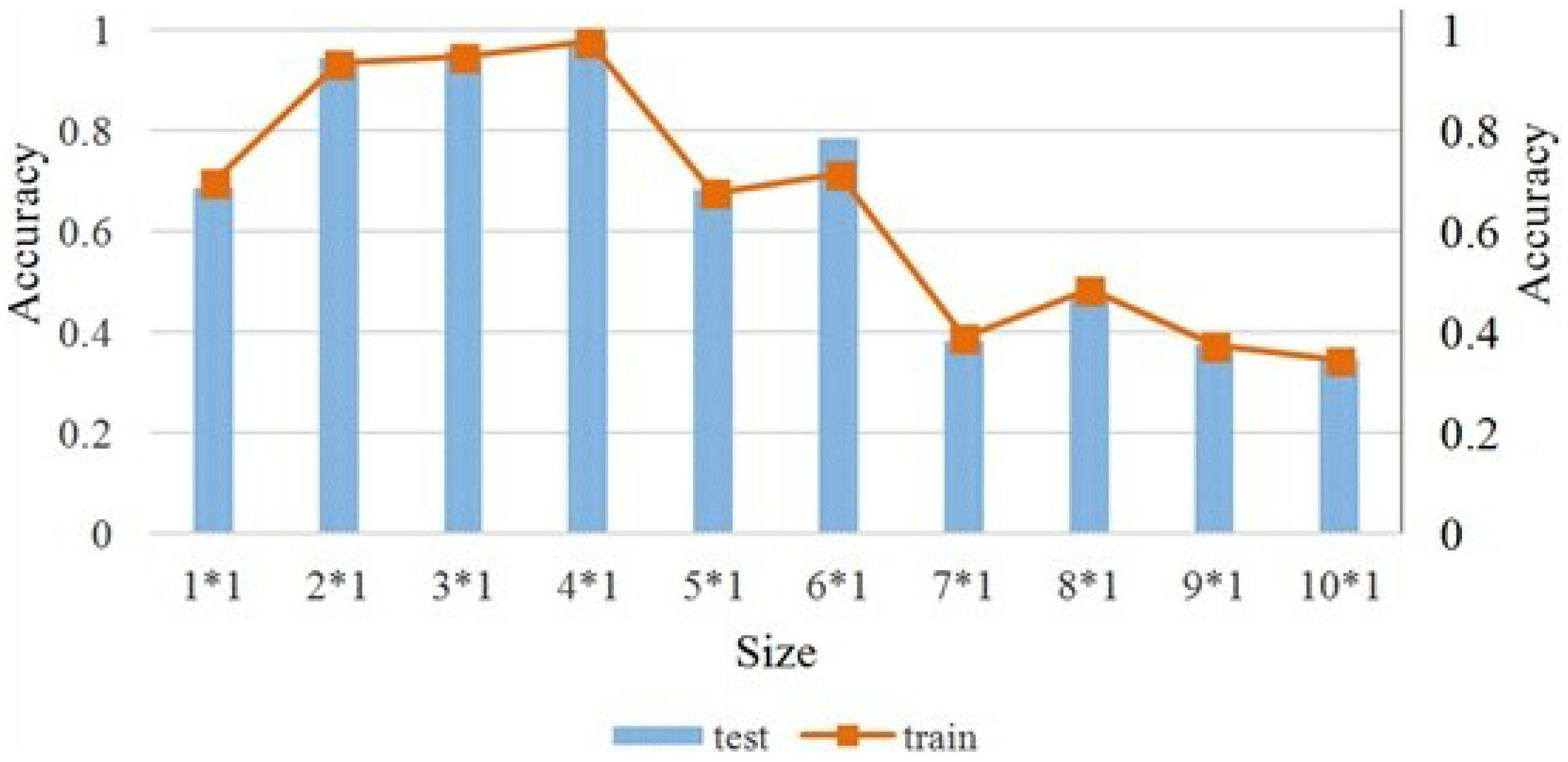
3.3. Performance of the First Convolutional Layer in Different Sizes of Convolution Kernels

Experiment 3 analyzed the performance of the first convolutional layer of ICECNN-1D in different sizes of convolution kernels. The first convolutional layer implemented convolution kernels with different sizes of 4*1, 8*1, 12*1, 16*1, 20*1, 24*1, 28*1, 32*1, 36*1 and 40*1 in the experiment. Other hyperparameters have not changed. The average accuracy rate is obtained as follows shown in Figure 7.

As shown in Figure 7, if the size of the convolution kernel in the first convolutional layer of ICECNN-1D model continued increasing, the overall training accuracy will also increase. The accuracy increased rapidly between 4*1 and 20*1, but when the convolution kernel reached a certain size, the test accuracy will decline and remain at a certain level. Analyzed result indicated the first convolution layer adopted an appropriate size convolution kernel (the convolution core with the size of "20 * 1" is selected in this study), which can increase network’s perception range and test recognition rate of time series data and learn characteristics of time series data efficiently.

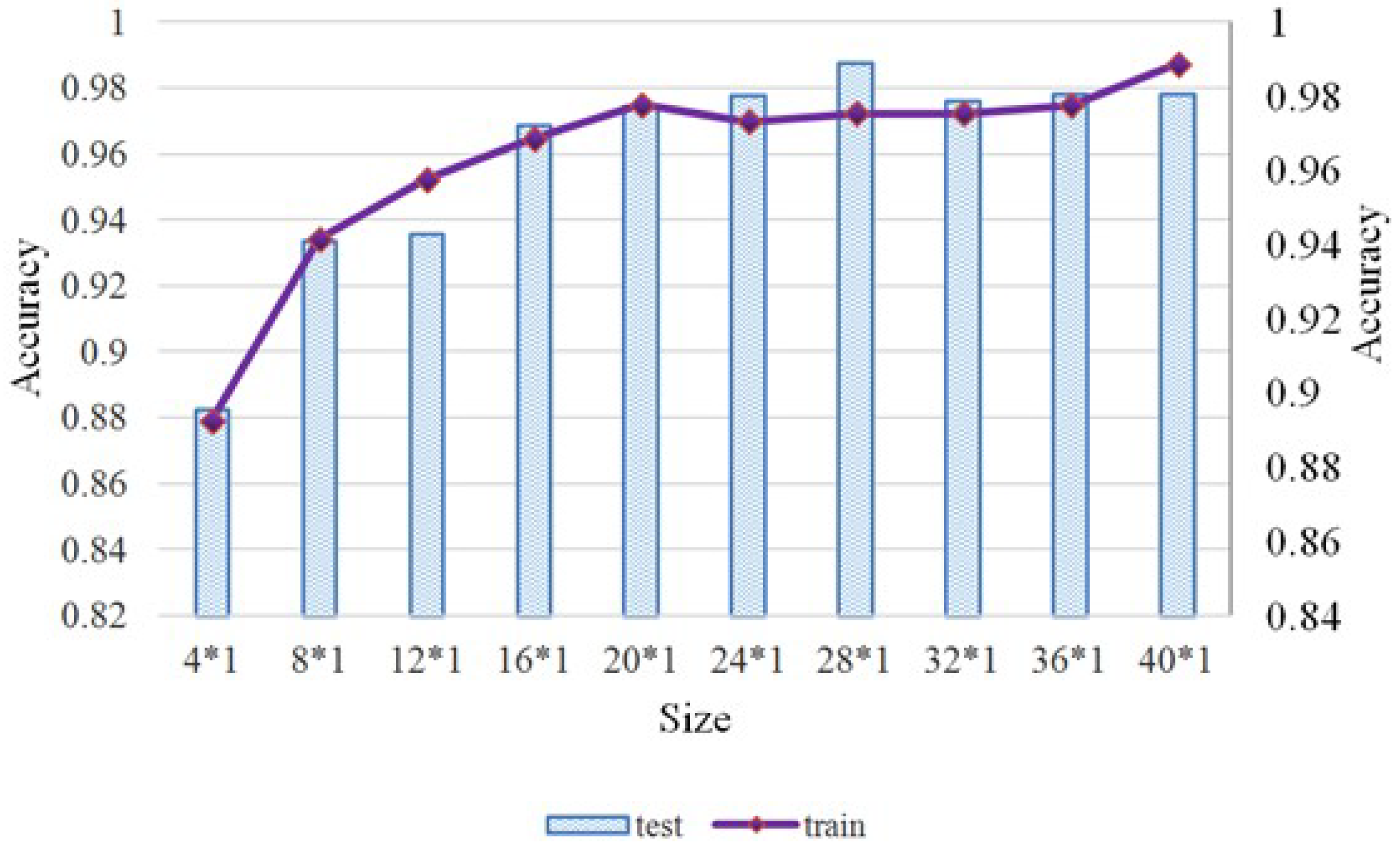
3.4. Experiment 4: Performance under Different Timing Input Widths

In experiment 4, time series signals with different length were implemented as the input of ICECNN-1D, CECNN-1D and NCNN-1D, and ability of model to perceive different widths of time series data was analyzed [30]. During the experiment, the collected data in one cycle was 512, and length of 512 was used as the signal length of one cycle (T). In data set A, the signal width of 1T to 10T is used as the input, The experimental results are shown in

Table 4. Experimental results under different timing widths of ICECNN-1D model.

Model ICECNN-1D	Recognition Accuracy (%)
Period (T)	1T	2T	3T	4T	5T
train	0.9577	0.9626	0.9763	0.9726	0.9791
test	0.9452	0.9594	0.9676	0.9742	0.9762
Period (T)	6T	7T	8T	9T	10T
train	0.9797	0.9796	0.9793	0.9782	0.9886
test	0.9749	0.9788	0.9723	0.9765	0.9781

,

Table 5. Experimental results under different timing widths of CECNN-1D model.

Model CECNN-1D	Recognition Accuracy (%)
Period (T)	1T	2T	3T	4T	5T
train	0.9576	0.9623	0.9754	0.9746	0.9789
test	0.9498	0.9572	0.9668	0.9730	0.9759
Period (T)	6T	7T	8T	9T	10T
train	0.9794	0.9794	0.9745	0.9714	0.9769
test	0.9721	0.9735	0.9715	0.9725	0.9779

and

Table 6. Experimental results under different timing widths of NCNN-1D model.

Model NCNN-ID	Recognition Accuracy (%)
Period (T)	1T	2T	3T	4T	5T
train	0.9445	0.9540	0.9627	0.9644	0.9659
test	0.9459	0.9465	0.9530	0.9422	0.9551
Period (T)	6T	7T	8T	9T	10T
train	0.9652	0.9677	0.9617	0.9647	0.9648
test	0.9540	0.9580	0.9589	0.9560	0.9539

.

As shown in Table 4, Table 5 and Table 6, the training and testing accuracy of NCNN-ID and CECNN-1D is lower than that of ICECNN-1D. As the input width increased from 1 cycle to 10 cycles, the training recognition rate and test recognition rate of ICECNN-1D model increased gradually. When the input reached 5 cycles, the recognition rate is high and it becomes basically stable. CECNN-1D has a certain fluctuation, while the accuracy of NCNN-1D test fluctuates greatly. Although there is an upward trend, the changes are not obvious, which indicated that the NCNN-ID model provides poor stability, poor performance in time series feature extraction, and weak generalization ability. However, ICECNN-ID model provided good performance to extract time series features, and the increase of the perception width could enhance the recognition rate.

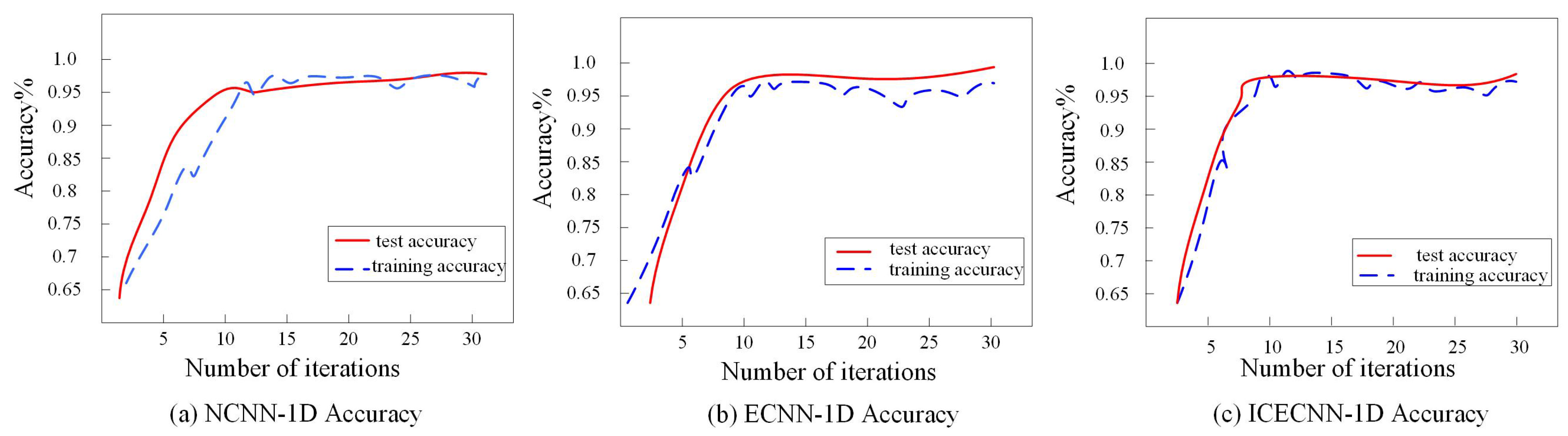
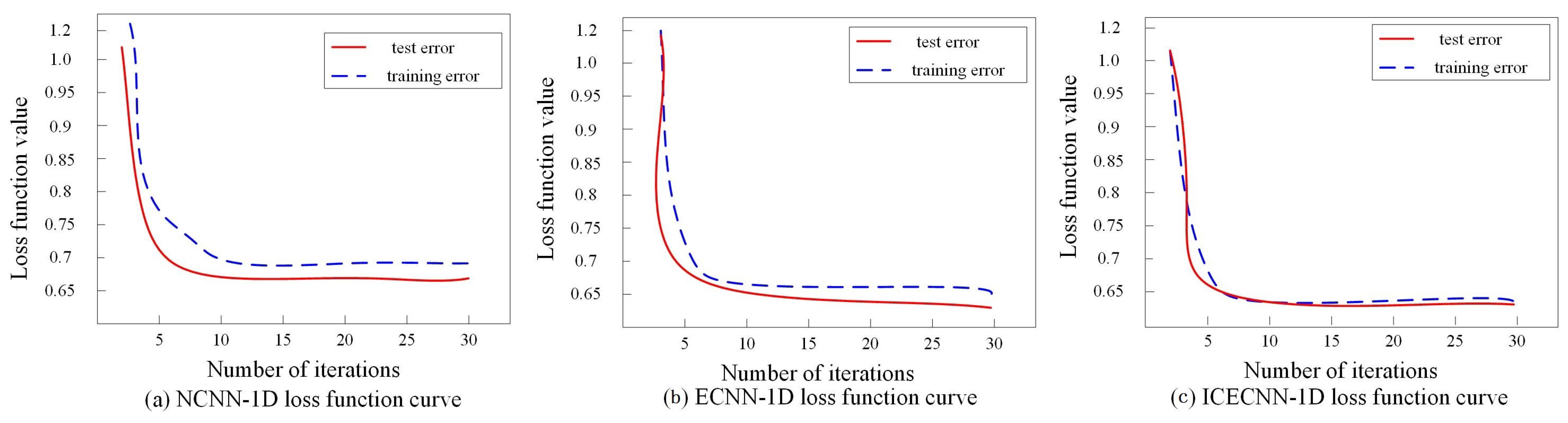
3.5. Experiment 5: Performance Comparison of Different Models

Experiment 5 compared several different machine algorithm models with the ICECNN-1D model, the one-dimensional machine learning (LetNet5-1D), AlexNet machine algorithm, VI-CNN, CECNN-1D and BP machine algorithm under the LetNet5 framework were applied for comparative experiments. To verify the generalization ability of the model, four kinds of data in A, B, C and D are used, and the experimental results of the average recognition rate and average training time are shown in

Table 7. Statistics of average recognition rate and average training time.

	Average Recognition Rate				Average Training Time (s)
	A	B	C	D
BPNN	78.86	74.33	75.79	78.15	132
LetNet5-1D	79.89	80.32	79.69	82.23	207
AlexNet-2D	86.64	89.59	88.66	87.26	225
VI-CNN	93.62	89.76	94.75	91.59	254
CECNN-1D	97.26	95.79	97.42	96.61	178
ICECNN-1D	97.55	97.86	97.89	97.84	167

.

Average accuracy of diagnosed results under 4 different loads was counted. According to Table 7, the recognition rates of BPNN, LetNet5-1D and AlexNet-2D are all below 90%. Additionally, VI-CNN machine algorithm provided a high recognition rate, but it provided undesirable ability of generation under different work condition because its recognition rate fluctuated obviously under different loads. CECNN-1D provides high recognition rate, but its recognition rate fluctuates under different loads and is lower than that of ICECNN-1D.The average training time of BPNN is the shortest, but the average recognition rate is also the lowest, but the average training time of ICECNN-1D is shorter than other algorithms, and the average recognition rate is the highest. Finally, results showed that ICECNN-1D provided ideal performance while processing high-frequency time series data, the indicated model also provided decent ability of generalization.

4. Conclusions

This paper introduced an intelligent fault diagnosis method by combining audio-visual fusion method and CNN. This method not only considers time series property while diagnosing faults but also considers the correlation between high-frequency signals and fault categories. Moreover, stability of introduced method was verified by analyzing fault diagnosis effects of rotor bearing with different loads. Accordingly, experimental results indicated ICECNN-1D provided reliable and accurate results to analyze time series signal while diagnosing faults. Moreover, considering problem that limited state information may increase the difficulty of analyzing multi-dimensional state information of electrical equipment, industrial instrument and mechanical equipment. Consequently, the proposed method fused audio and visual information to effectively utilize information in the time series signals, which improve the efficiency of diagnosing faults.

This study only analyzes the rotor bearing pitting fault. Therefore, in the future work, we will further study the fault diagnosis of rotor bearings under different loads, different fault types and multiple fault modes, and use the proposed method to conduct in-depth research on early fault diagnosis of bearings; In addition, we will continue to deeply study the color histogram theory of one-dimensional signals, carry out experiments from the aspect of signal vision, so as to provide a comprehensive and ideal solution for the fault diagnosis of electrical equipment, industrial instruments and mechanical equipment.

References

1. Fan, L.; Chai, Y.; Chen, X. Trend attention fully convolutional network for remaining useful life estimation. Reliab. Eng. Syst. Saf. 2022, 225, 108590. [Google Scholar] [CrossRef]
2. Chen, H.; Jiang, B.; Ding, S.X.; Huang, B. Data-driven fault diagnosis for traction systems in high-speed trains: A survey, challenges and perspectives. IEEE Trans. Intell. Transp. Syst. 2020, 23, 1700–1716. [Google Scholar] [CrossRef]
3. Xu, S.; Tao, S.; Zheng, W.; Chai, Y.; Ma, M.; Ding, L. Multiple open-circuit fault diagnosis for back-to-back converter of PMSG wind generation system based on instantaneous amplitude estimation. IEEE Trans. Instrum. Meas. 2021, 70, 1–13. [Google Scholar] [CrossRef]
4. Xu, S.; Huang, W.; Wang, H.; Zheng, W.; Wang, J.; Chai, Y.; Ma, M. A Simultaneous Diagnosis Method for Power Switch and Current Sensor Faults in Grid-Connected Three-Level NPC Inverters. IEEE Trans. Power Electron. 2022, 38, 1104–1118. [Google Scholar] [CrossRef]
5. Guo, Q. Research on the application of improved shuffled frog leaping algorithm in mechanical fault diagnosis. Acad. J. Manuf. Eng. 2018, 16, 137–142. [Google Scholar]
6. Ziani, R.; Felkaoui, A.; Zegadi, R. Bearing fault diagnosis using multiclass support vector machines with binary particle swarm optimization and regularized Fisher’s criterion. J. Intell. Manuf. 2017, 28, 405–417. [Google Scholar] [CrossRef]
7. Niu, Q. Discussion on fault diagnosis of and solution seeking for rolling bearing based on deep learning. Acad. J. Manuf. Eng. 2018, 16, 58–64. [Google Scholar]
8. Shi, L.; Zhu, Y.; Zhang, Y.; Su, Z. Fault Diagnosis of Signal Equipment on the Lanzhou-Xinjiang High-Speed Railway Using Machine Learning for Natural Language Processing. Complexity 2021, 2021, 9126745. [Google Scholar] [CrossRef]
9. Buczak, A.L.; Guven, E. A Survey of Data Mining and Machine Learning Methods for Cyber Security Intrusion Detection. IEEE Commun. Surv. Tutorials 2017, 18, 1153–1176. [Google Scholar] [CrossRef]
10. Liu, B.; Chai, Y.; Huang, C.; Fang, X.; Tang, Q.; Wang, Y. Industrial process monitoring based on optimal active relative entropy components. Measurement 2022, 197, 111160. [Google Scholar] [CrossRef]
11. Ren, H.; Qu, J.F.; Chai, Y.; Tang, Q.; Ye, X. Deep learning for fault diagnosis: The state of the art and challenge. Control. Decis. 2017, 32, 1345–1358. [Google Scholar]
12. Abid, F.B.; Sallem, M.; Braham, A. Robust Interpretable Deep Learning for Intelligent Fault Diagnosis of Induction Motors. IEEE Trans. Instrum. Meas. 2019, 69, 3506–3515. [Google Scholar] [CrossRef]
13. Chen, H.; Chen, Z.; Chai, Z.; Jiang, B.; Huang, B. A single-side Neural Network-aided canonical correlation analysis with applications to fault diagnosis. IEEE Trans. Cybern. 2021, 52, 9454–9466. [Google Scholar] [CrossRef] [PubMed]
14. Liang, X.; Wang, H.F.; Guo, J.; Xu, T.H. Bayesian Network Based Fault Diagnosis Method for On-board Equipment of Train Control System. J. China Railw. Soc. 2017, 39, 93–100. [Google Scholar]
15. An, P. Fault diagnosis method of mechanical hydraulic system based on artificial intelligence. Acad. J. Manuf. Eng. 2017, 15, 55–59. [Google Scholar]
16. Lu, Q.; Al-Wahaibi, S.S. Enhanced CNN with Global Features for Fault Diagnosis of Complex Chemical Processes. arXiv 2022, arXiv:2210.01727. [Google Scholar]
17. Jiang, X.; Yang, S.; Wang, F.; Xu, S.; Wang, X.; Cheng, X. OrbitNet: A new CNN model for automatic fault diagnostics of turbomachines. Appl. Soft Comput. 2021, 110, 107702. [Google Scholar] [CrossRef]
18. Zhang, X.; Wang, H.; Wu, B.; Zhou, Q.; Hu, Y. A novel data-driven method based on sample reliability assessment and improved CNN for machinery fault diagnosis with non-ideal data. J. Intell. Manuf. 2022, 1–14. [Google Scholar] [CrossRef]
19. Park, C.H.; Kim, H.; Lee, J.; Ahn, G.; Youn, M.; Youn, B.D. A Feature Inherited Hierarchical Convolutional Neural Network (FI-HCNN) for Motor Fault Severity Estimation Using Stator Current Signals. Korean Soc. Precis. Eng. 2021, 8, 1253–1266. [Google Scholar] [CrossRef]
20. Deng, H.; Zhang, W.X.; Liang, Z.F. Application of BP Neural Network and Convolutional Neural Network (CNN) in Bearing Fault Diagnosis. IOP Conf. Ser. Mater. Sci. Eng. 2021, 1043, 042026. [Google Scholar] [CrossRef]
21. Li, H. Computer network connection enhancement optimization algorithm based on convolutional Neural Network. In Proceedings of the 2021 International Conference on Networking, Communications and Information Technology (NetCIT), Manchester, UK, 26–27 December 2021; pp. 281–284. [Google Scholar]
22. Shoka, A.A.E.; Dessouky, M.M.; El-Sayed, A.; Hemdan, E.E.D. An Efficient CNN Based Epileptic Seizures Detection Framework Using Encrypted EEG Signals for Secure Telemedicine Applications. Alex. Eng. J. 2022, in press. [Google Scholar]
23. Brynjolfsson, E.; Mitchell, T. What can machine learning do? Workforce implications. Science 2017, 358, 1530–1534. [Google Scholar] [CrossRef]
24. Gastegger, M.; Behler, J.; Marquet, P. Machine Learning Molecular Dynamics for the Simulation of Infrared Spectra. Chem. Sci. 2017, 8, 6924–6935. [Google Scholar] [CrossRef] [Green Version]
25. Lamperti, F.; Roventini, A.; Sani, A. Agent-Based Model Calibration using Machine Learning Surrogates. J. Econ. Dyn. Control. 2018, 90, 366–389. [Google Scholar] [CrossRef] [Green Version]
26. Zhang, J.; Wang, Z.; Verma, N. In-Memory Computation of a Machine-Learning Classifier in a Standard 6T SRAM Array. IEEE J. Solid-State Circuits 2017, 52, 915–924. [Google Scholar] [CrossRef]
27. Liu, Y.; Chai, Y.; Liu, B.; Wang, Y. Bearing Fault Diagnosis Based on Energy Spectrum Statistics and Modified Mayfly Optimization Algorithm. Sensors 2021, 21, 2245. [Google Scholar] [CrossRef] [PubMed]
28. Goodfellow, I.; McDaniel, P.; Papernot, N. Making Machine Learning Robust Against Adversarial Inputs. Commun. ACM 2018, 61, 56–66. [Google Scholar] [CrossRef]
29. Char, D.S.; Shah, N.H.; Magnus, D. Implementing Machine Learning in Health Care - Addressing Ethical Challenges. N. Engl. J. Med. 2018, 378, 981–983. [Google Scholar] [CrossRef] [Green Version]
30. Assouline, D.; Mohajeri, N.; Scartezzini, J.L. Quantifying rooftop photovoltaic solar energy potential: A machine learning approach. Solar Energy 2017, 141, 278–296. [Google Scholar] [CrossRef]
Figure 1. ICECNN-1D Neural Network structure.
Electronics 11 04207 g001
Figure 2. Flow chart of diagnosing faults.
Electronics 11 04207 g002
Figure 3. Fault data of inner race of drive end bearing under different loads.
Electronics 11 04207 g003
Figure 4. The accuracy trend of three models’ function.
Electronics 11 04207 g004
Figure 5. Trend chart of the three models’ loss function.
Electronics 11 04207 g005
Figure 6. Accuracy statistics at different compression sizes.
Electronics 11 04207 g006
Figure 7. Accuracy statistics for different convolution kernel sizes.
Electronics 11 04207 g007