CNN-Based Fluid Motion Estimation Using Correlation Coefficient and Multiscale Cost Volume

Abstract

Motion estimation for complex fluid flows via their image sequences is a challenging issue in computer vision. It plays a significant role in scientific research and engineering applications related to meteorology, oceanography, and fluid mechanics. In this paper, we introduce a novel convolutional neural network (CNN)-based motion estimator for complex fluid flows using multiscale cost volume. It uses correlation coefficients as the matching costs, which can improve the accuracy of motion estimation by enhancing the discrimination of the feature matching and overcoming the feature distortions caused by the changes of fluid shapes and illuminations. Specifically, it first generates sparse seeds by a feature extraction network. A correlation pyramid is then constructed for all pairs of sparse seeds, and the predicted matches are iteratively updated through a recurrent neural network, which lookups a multi-scale cost volume from a correlation pyramid via a multi-scale search scheme. Then it uses the searched multi-scale cost volume, the current matches, and the context features as the input features to correlate the predicted matches. Since the multi-scale cost volume contains motion information for both large and small displacements, it can recover small-scale motion structures. However, the predicted matches are sparse, so the final flow field is computed by performing a CNN-based interpolation for these sparse matches. The experimental results show that our method significantly outperforms the current motion estimators in capturing different motion patterns in complex fluid flows, especially in recovering some small-scale vortices. It also achieves state-of-the-art evaluation results on the public fluid datasets and successfully captures the storms in Jupiter’s White Ovals from the remote sensing images.

1. Introduction

Motion estimation for complex fluid flows via their image sequences is a challenging problem in computer vision. It plays an important role in scientific research and engineering applications related to meteorology, oceanography, and fluid mechanics, such as the analysis of atmospheric or sea ice motion, the detection and early warning of a forest fire or smoke, the prediction of sandstorms or tornadoes, the application of particle image velocimetry, etc. It provides reliable measurement in a non-intrusive way to acquire a deeper insight of complex flow phenomena. During the last several decades, although a great many motion estimators [1,2,3,4,5,6,7,8] have been introduced to predict the motion of complex fluid flows, there are still some challenging problems that need to be solved.

The fluid is nonrigid and characterized by hardly predictable variation. When the fluid flows from one image to another, its shape often changes. Therefore, how to over-come the change of fluid shapes with time is the key for high-precision fluid motion estimation. In addition, the fluid is usually transparent and contains weak textures. Different parts of the fluid often have a similar appearance. Therefore, it is difficult to distinguish the differences between them. Furthermore, when the fluid is affected by the illumination changes, its brightness often changes. This leads to ambiguity in the matching between different parts of a fluid image pair. Therefore, how to enhance the discriminability for them is another challenge of high-precision fluid motion estimation. Finally, the fluid flows generally contain complex motion patterns, the current motion estimators [9,10,11] often fail to capture them, especially when recovering some small-scale motion structures. Therefore, how to capture these different motion patterns in complex fluid flows is another urgent problem that needs to be solved.

In this paper, we solve these problems by introducing a novel motion estimator, and the main contributions are summarized as follows:

• A novel CNN-based motion estimator is introduced to predict complex fluid flows, and it uses correlation coefficients as the matching costs, which can overcome the feature distortions caused by the changes of fluid shapes and illuminations, and improve the accuracy of motion estimation by enhancing the discrimination of the feature matching.
• The multi-scale cost volume is retrieved from a correlation pyramid using a multi-scale search scheme. Therefore, it contains both global and local motion information, which can recover the moving structures with both large and small displacements and, especially capture the motion of small fast-moving objects, such as some important small-scale vortices in complex fluid flows.
• The proposed CNN-based motion estimator significant outperforms the current optical flow methods in capturing different motion patterns in complex fluid flows. It also achieves state-of-the-art evaluation results on the public fluid datasets and successfully captures the storms in Jupiter’s White Ovals from the remote sensing images.

2. Related Work

In this section, we briefly review the motion estimators related to the complex fluid flows. During the past several decades, various motion estimators have been developed to improve the accuracy of fluid motion estimation. These methods are mainly classified into three groups: correlation-based methods, variational optical flow methods, and CNN-based motion estimators.

2.1. Correlation-Based Methods

The traditional correlation-based method [1] divides an image into many interrogation windows with a fixed size, and it finds the best match by searching for the maximum of cross-correlation between two interrogation windows of an image pair. However, it often produces sparse matches and requires a post-processing step, such as outlier detection and interpolation. Then, a great many methods have been proposed to solve this problem. Astarita et al. [2,3] improved the spatial resolution of the velocity field by a velocity interpolation and image deformation. Becker et al. [4] proposed a variational adaptive correlation method, which predicts complex fluid flows using a variational adaptive Gaussian window. Theunissen et al. [5] introduced an adaptive sampling and windowing interrogation method to improve the robustness of particle image velocimetry. They later [6] proposed a spatially adaptive PIV interrogation based on the data ensemble to select the adaptive interrogation parameters. Yu et al. [7] proposed an adaptive PIV algorithm based on seeding density and velocity information. Although correlation-based methods have greatly improved over the last several decades, they still have relatively large errors in regions with large velocity gradients due to the smoothing effect of the interrogation window.

2.2. Variational Optical Flow Methods

To overcome the shortcomings of correlation-based methods, variational optical flow methods are introduced to acquire the dense velocity fields. The variational optical flow model was first proposed by Horn and Schunck [8], and it relies on the energy minimization of an objective function that consists of a data term and a regularization term. The data term is associated with the brightness constancy assumption, which assumes that when a pixel flows from one image to another, its brightness does not change. However, the brightness constancy assumption is sensitive to illumination changes in the real world. At the same time, the regularization term uses the penalization of the $\mathrm{L}2$ norm, which leads to an isotropic diffusion that can yield over-smoothing flow fields in motion discontinuities. Therefore, a great many optical flow methods are introduced to solve these problems. Brox et al. [12] added the gradient constancy assumption to the data term to handle weak illumination changes and introduced a robust penalty function for the regularization term that can create piecewise smooth flow fields. An isotropic TV-$\mathrm{L}1$ regularization was first proposed by Zach et al. [13] to preserve motion discontinuities. Corpetti et al. [14] investigated a dedicated minimization-based motion estimator, and the cost function includes a novel data term relying on an integrated version of the continuity equation of fluid mechanics, which is associated with an original second-order div-curl regularizer. Zhou et al. [15] presented a novel approach to estimate and analyze the 3D fluid structure and motion of clouds from multi-spectrum 2D cloud image sequences. Sakaino [16] introduced optical flow estimation based on the physical properties of waves and later proposed a spatiotemporal image pattern prediction method [17] based on a physical model with a time-varying optical flow. Li et al. [18] proposed to recover fluid-type motions using a Navier–Stokes potential flow. Cuzol et al. [19] proposed a new motion estimator for image sequences depicting fluid flows, relying on the Helmholtz decomposition of a motion field, which consists of decoupling the velocity field into a divergence free component and a vorticity free component. Ren et al. [20] proposed a novel incompressible SPH solver, where the compressibility of fluid is directly measured by the deformation gradient. Although these motion estimators improve the accuracy of the fluid motion estimation, they still do not handle the feature distortions caused by the changes of fluid shapes and illuminations, and also do not capture some important small-scale motion structures.

2.3. CNN-Based Motion Estimators

In recent work, convolutional neural networks have attracted a great deal of attention due to their remarkable success in computer vision. FlowNet [21] is the first end-to-end supervised optical flow learning framework, which takes an image pair as the input and outputs a dense flow field. FlowNet2 [22] is later proposed to improve the accuracy by staking several basic FlowNet modules for refinement. PWC-Net [23] computes optical flow with CNNs via a pyramid, warping, and cost volume. LiteFlowNet [24] achieves start-of-the-art results with a lightweight framework by warping the features extracted from CNNs. ARFlow [25] introduces an unsupervised optical flow estimation by the reliable supervision from transformations. RAFT [11] is a new deep network architecture for optical flow estimation using recurrent all-pairs field transformations. GMA [26] solves the occlusion problem by introducing a global motion aggregation module. Recently, Cai et al. [9] proposed the dense motion estimation of particle images via a convolutional neural network base on FlowNetS [21], and the corresponding CNN model is trained with a synthetic dataset of fluid flow images. They later [10] introduced an enhanced configuration of LiteFlowNet [24] for particle image velocimetry, which achieves a high accuracy via training the corresponding CNN model using different kinds of fluid-like images. However, these CNN-based motion estimators do not outperform the well-established correlation-based optical flow methods for all aspects, and the accuracy of them is largely determined by the training data. Masaki et al. [27] introduced convolutional neural networks for fluid flow analysis, toward effective metamodeling and low-dimensionalization. It considers two types of CNN-based fluid flow analyses: CNN metamodeling and CNN autoencoder. For the first type of CNN, which has additional scalar inputs, they investigated the influence of the input placements in the CNN training pipeline, and then investigated the influence of the various parameters and operations on CNN performance, with the utilization of an autoencoder. Murata et al. [28] proposed a nonlinear mode decomposition with convolutional neural networks for fluid dynamics, which is used to visualize decomposed flow fields. Nakamura et al. [29] introduced a robust training approach for neural networks for fluid flow state estimations, where a convolutional neural network is utilized to estimate velocity fields from sectional sensor measurements. Yu et al. [30] proposed a cascaded convolutional neural network to implement end-to-end two-phase flow fluid motion estimation. Liang et al. [31] introduced particle-tracking velocimetry for complex flow motion via deep neural networks, which has a high accuracy and efficiency. Guo et al. [32] proposed a time-resolved particle image velocimetry algorithm based on deep learning, which achieves excellent performance with a competitive calculation accuracy and high calculation efficiency. In contrast with these existing CNN-based methods [27,28,29,30,31,32] for fluid flow estimation, our method uses a very different network structure, which uses correlation coefficients as the matching costs to enhance the discrimination of the feature matching and overcome the feature distortions caused by the changes of fluid shapes and illuminations, and it also achieves state-of-the-art results on the public fluid datasets.

3. Proposed Approach

3.1. Overview

In this section, a novel CNN-based motion estimator is introduced to predict complex fluid flows. It mainly consists of five parts: (1) sparse seeds; (2) a correlation pyramid; (3) multi-scale cost volume; (4) a CNN-based update module; (5) CNN-based interpolation. Next, we will introduce each part in detail.

3.2. Sparse Seeds

A dense motion field is predicted by first generating sparse seeds on the image plane. This is based on the observation that the motion field is generally sparse due to the motion self-similarity of pixels in a local neighborhood. Therefore, it is unnecessary to compute the match for each pixel. Specifically, by selecting appropriate seeds on the image plane, the computational efficiency for optical flow estimation can be greatly improved with almost no loss in accuracy. After obtaining matches for the sparse seeds, a CNN-based interpolation is performed to recover the sparse matches to the full resolution.

The sparse seeds are generated by a feature extraction network, and seeds $S_1$ and $S_2$ are extracted from input image pair $I_1$ and $I_2$, respectively, with the resolution of W × H and three color channels, where W and H are the width and height of the image, respectively. Specifically, this feature extraction network consists of a convolution layer, 2n residual blocks (where every two residual blocks is a group, and the resolution of each residual block in the k-th group is $\raisebox{1ex}{$\mathrm{W}$}\!\left/ \!\raisebox{-1ex}{$2^{\mathrm{k}}$}\right.\times \raisebox{1ex}{$\mathrm{H}$}\!\left/ \!\raisebox{-1ex}{$2^{\mathrm{k}}$}\right.$), and a convolution layer, where k = 1,2,…,n. The sparse seeds are the output features of the feature extraction network, where the adjacent seeds have an interval of n pixels. The sparsity of seeds is controlled by adjusting the interval n, which is often set to 2 or 3 in practice. Since these sparse seeds are evenly distributed on the image plane at equal intervals, it ensures enough matches in a local neighborhood. It is very helpful for our method to better restore local motion details by a CNN-based interpolation.

$F_s$ and $F_t$ are the feature maps for the seeds $S_1$ and $S_2$, respectively, which are extracted from a pair of images $I_1$ and $I_2$ using the same feature extraction network in Figure 1. In addition, the context feature map $F_c$ is extracted from the first input image $I_1$ using the context network, which is the same as the feature extraction network. The structure of the feature extraction network is given in Figure 1. The context feature map is mainly used as a guide to preserve the motion discontinuities for the optical flow field to be estimated. This is based on the observation that motion boundaries are often consistent with the edge structures of the input image $I_1$.

3.3. Correlation Pyramid

Inspired by the properties of correlation coefficients, we construct a full correlation volume by computing correlation coefficients between all the feature pairs of ${\mathrm{F}}_{\mathrm{s}}$ and ${\mathrm{F}}_{\mathrm{t}}$, where the size of ${\mathrm{F}}_{\mathrm{s}}$ and ${\mathrm{F}}_{\mathrm{t}}$ is ${\mathrm{W}}_{\mathrm{s}}\times {\mathrm{H}}_{\mathrm{s}}=\raisebox{1ex}{$\mathrm{W}$}\!\left/ \!\raisebox{-1ex}{$2^{\mathrm{n}}$}\right.\times \raisebox{1ex}{$\mathrm{H}$}\!\left/ \!\raisebox{-1ex}{$2^{\mathrm{n}}$}\right.$. Specifically, the correlation coefficients are used as the matching costs, and the matching cost between two feature vectors, ${\mathrm{F}}_{\mathrm{s}}\left(\mathrm{x}\right)$ located at $\mathrm{x}$ and ${\mathrm{F}}_{\mathrm{t}}\left(\mathrm{y}\right)$ located at $\mathrm{y}$, is computed by:

$$\mathrm{C}\left({\mathrm{F}}_{\mathrm{s}}\left(\mathrm{x}\right),{\mathrm{F}}_{\mathrm{t}}\left(\mathrm{y}\right)\right)=\frac{1}{\mathrm{D}}{\displaystyle \sum }_{\mathrm{h}=1}^{\mathrm{D}}\frac{{\mathrm{F}}_{\mathrm{s}}^{\mathrm{h}}\left(\mathrm{x}\right)-{\mathsf{\mu }}_{\mathrm{s}}\left(\mathrm{x}\right)}{{\mathsf{\sigma }}_{\mathrm{s}}\left(\mathrm{x}\right)}·\frac{{\mathrm{F}}_{\mathrm{t}}^{\mathrm{h}}\left(\mathrm{y}\right)-{\mathsf{\mu }}_{\mathrm{t}}\left(\mathrm{y}\right)}{{\mathsf{\sigma }}_{\mathrm{t}}\left(\mathrm{y}\right)}$$

(1)

where $\mathrm{h}\in \left\{1,2,\dots ,\mathrm{D}\right\}$ is the channel index, and ${\mathsf{{\rm M}}}_{\mathrm{s}}\left(\mathrm{x}\right)$, ${\mathsf{\mu }}_{\mathrm{t}}\left(\mathrm{y}\right)$ and ${\mathsf{\sigma }}_{\mathrm{s}}\left(\mathrm{x}\right)$, ${\mathsf{\sigma }}_{\mathrm{t}}\left(\mathrm{y}\right)$ are the means and variances of the feature vectors ${\mathrm{F}}_{\mathrm{s}}\left(\mathrm{x}\right)$, ${\mathrm{F}}_{\mathrm{t}}\left(\mathrm{y}\right)$ along the channel, respectively.

For a feature vector in ${\mathrm{F}}_{\mathrm{s}}$, we take the matching costs between it and all the feature vectors in ${\mathrm{F}}_{\mathrm{t}}$ to generate a 2D ${\mathrm{W}}_{\mathrm{s}}\times {\mathrm{H}}_{\mathrm{s}}$ correlation map. That is, each feature vector in ${\mathrm{F}}_{\mathrm{s}}$ produces a 2D response map. Therefore, a full correlation volume is a 4D ${\mathrm{W}}_{\mathrm{s}}\times {\mathrm{H}}_{\mathrm{s}}\times {\mathrm{W}}_{\mathrm{s}}\times {\mathrm{H}}_{\mathrm{s}}$ volume, which is formed by taking the matching costs between all the feature pairs of ${\mathrm{F}}_{\mathrm{s}}$ and ${\mathrm{F}}_{\mathrm{t}}$. As in [11], a correlation pyramid $C=\left\{{\mathrm{C}}^{\mathrm{l}}|\mathrm{l}=0,1,\dots ,\mathrm{L}-1\right\}$ is constructed by an average pooling for the last two dimensions of the correlation volume with a kernel size of $\mathsf{\kappa }=\left\{2^{\left(\mathrm{l}\right)}\times 2^{\left(\mathrm{l}\right)}|\mathrm{l}=0,1,\dots ,\mathrm{L}-1\right\}$, where ${\mathrm{C}}^{\left(\mathrm{l}\right)}$ has a dimension of ${\mathrm{H}}_{\mathrm{s}}\times {\mathrm{W}}_{\mathrm{s}}\times \raisebox{1ex}{${\mathrm{H}}_{\mathrm{s}}$}\!\left/ \!\raisebox{-1ex}{$2^{\mathrm{l}}$}\right.\times \raisebox{1ex}{${\mathrm{W}}_{\mathrm{s}}$}\!\left/ \!\raisebox{-1ex}{$2^{\mathrm{l}}$}\right.$. The correlation pyramid is a multi-scale correlation volume, which contains coarse-to-fine correlation features about almost all the different displacements of sparse seeds, and we can look up the matching costs of different displacements at different scales for a feature vector in $F_s$ from the correlation pyramid. Since the correlation pyramid considers both low- and high-resolution correlation information, while maintaining the first two dimensions (or the full resolution) of sparse seeds $S_1$, it allows for our method to recover both large and small displacements, especially to capture the motion of small fast-moving objects, such as small-scale vortices in complex fluid flows.

Now, let us discuss the advantages of the multi-scale correlation volume using correlation coefficients as the matching costs.

3.3.1. Feature-Distortion Invariance

When the fluid flows from one image to another, its shape is often not fixed, and it tends to change with time, such as local contraction and expansion. At the same time, its brightness often changes due to the influence of illumination changes. Therefore, the extracted features are often distorted to some extent. We maintain feature-distortion invariance by using correlation coefficients as the matching costs. ${\mathrm{F}}_{\mathrm{s}}\left(\mathrm{x}\right)$ is a feature vector of a seed located at $\mathrm{x}$ in the source feature map $S_1$, when this seed moves from the source feature map $S_1$ to the target feature map $S_2$, its feature may be distorted due to the changes of fluid shapes and illuminations. We assume that it satisfies the following feature-distortion model:

$${\mathrm{F}}_{\mathrm{i}}\left(\mathrm{y}\right)={\mathrm{a}}_{\mathrm{y}}{\mathrm{F}}_{\mathrm{t}}\left(\mathrm{y}\right)+{\mathrm{b}}_{\mathrm{y}}$$

(2)

where ${\mathrm{F}}_{\mathrm{t}}\left(\mathrm{y}\right)$ denotes an original feature vector in the target feature map ${\mathrm{S}}_2$, and ${\mathrm{F}}_{\mathrm{i}}\left(\mathrm{y}\right)$ is the corresponding feature vector influenced by the changes of fluid shapes and illuminations. ${\mathrm{a}}_{\mathrm{y}}$ and ${\mathrm{b}}_{\mathrm{y}}$ represent the parameters of this linear model located at $\mathrm{y}$. The mean ${\mathsf{\mu }}_{\mathrm{i}}\left(\mathrm{y}\right)$ and standard deviation ${\mathsf{\sigma }}_{\mathrm{i}}\left(\mathrm{y}\right)$ of ${\mathrm{F}}_{\mathrm{i}}\left(\mathrm{y}\right)$ can be respectively given by:

$${\mathsf{\mu }}_{\mathrm{i}}\left(\mathrm{y}\right)={\mathrm{a}}_{\mathrm{y}}{\mathsf{\mu }}_{\mathrm{t}}\left(\mathrm{y}\right)+{\mathrm{b}}_{\mathrm{y}}$$

(3)

$${\mathsf{\sigma }}_{\mathrm{i}}\left(\mathrm{y}\right)={\mathrm{a}}_{\mathrm{y}}{\mathsf{\sigma }}_{\mathrm{t}}\left(\mathrm{y}\right)$$

(4)

where ${\mathsf{\sigma }}_{\mathrm{t}}\left(\mathrm{y}\right)$ and ${\mathsf{\mu }}_{\mathrm{t}}\left(\mathrm{y}\right)$ are the standard and mean deviation of ${\mathrm{F}}_{\mathrm{t}}\left(\mathrm{y}\right)$, respectively. Based on Equations (1)–(4), the matching cost between ${\mathrm{F}}_{\mathrm{s}}\left(\mathrm{x}\right)$ and ${\mathrm{F}}_{\mathrm{i}}\left(\mathrm{y}\right)$ is given by:

$$\begin{gathered} \mathrm{C}\left({\mathrm{F}}_{\mathrm{s}}\left(\mathrm{x}\right),{\mathrm{F}}_{\mathrm{t}}\left(\mathrm{y}\right)\right)=\mathrm{C}\left({\mathrm{F}}_{\mathrm{s}}\left(\mathrm{x}\right),{\mathrm{a}}_{\mathrm{y}}{\mathrm{F}}_{\mathrm{t}}\left(\mathrm{y}\right)+{\mathrm{b}}_{\mathrm{y}}\right) \\ =\frac{1}{\mathrm{D}}{\displaystyle \sum }_{\mathrm{h}=1}^{\mathrm{D}}\frac{{\mathrm{F}}_{\mathrm{s}}^{\mathrm{h}}\left(\mathrm{x}\right)-{\mathsf{\mu }}_{\mathrm{s}}\left(\mathrm{x}\right)}{{\mathsf{\sigma }}_{\mathrm{s}}\left(\mathrm{x}\right)}·\frac{{\mathrm{F}}_{\mathrm{i}}^{\mathrm{h}}\left((\mathrm{y}\right))-{\mathsf{\mu }}_{\mathrm{i}}\left(\mathrm{y}\right)}{{\mathsf{\sigma }}_{\mathrm{i}}\left(\mathrm{y}\right)} \\ =\frac{1}{\mathrm{D}}{\displaystyle \sum }_{\mathrm{h}=1}^{\mathrm{D}}\frac{{\mathrm{F}}_{\mathrm{s}}^{\mathrm{h}}\left(\mathrm{x}\right)-{\mathsf{\mu }}_{\mathrm{s}}\left(\mathrm{x}\right)}{{\mathsf{\sigma }}_{\mathrm{s}}\left(\mathrm{x}\right)}·\frac{{\mathrm{a}}_{\mathrm{y}}{\mathrm{F}}_{\mathrm{t}}^{\mathrm{h}}\left(\mathrm{y}\right)+{\mathrm{b}}_{\mathrm{y}}-\left({\mathrm{a}}_{\mathrm{y}}{\mathsf{\mu }}_{\mathrm{t}}\left(\mathrm{y}\right)+{\mathrm{b}}_{\mathrm{y}}\right)}{{\mathrm{a}}_{\mathrm{y}}{\mathsf{\sigma }}_{\mathrm{t}}\left(\mathrm{y}\right)} \\ =\frac{1}{\mathrm{D}}{\displaystyle \sum }_{\mathrm{h}=1}^{\mathrm{D}}\frac{{\mathrm{F}}_{\mathrm{s}}^{\mathrm{h}}\left(\mathrm{x}\right)-{\mathsf{\mu }}_{\mathrm{s}}\left(\mathrm{x}\right)}{{\mathsf{\sigma }}_{\mathrm{s}}\left(\mathrm{x}\right)}·\frac{{\mathrm{F}}_{\mathrm{t}}^{\mathrm{h}}\left((\mathrm{y}\right))-{\mathsf{\mu }}_{\mathrm{t}}\left(\mathrm{y}\right)}{{\mathsf{\sigma }}_{\mathrm{t}}\left(\mathrm{y}\right)}=\mathrm{C}\left({\mathrm{F}}_{\mathrm{s}}\left(\mathrm{x}\right),{\mathrm{F}}_{\mathrm{t}}\left(\mathrm{y}\right)\right) \end{gathered}$$

(5)

which demonstrates that although the feature vector ${\mathrm{F}}_{\mathrm{i}}\left(\mathrm{y}\right)={\mathrm{a}}_{\mathrm{y}}{\mathrm{F}}_{\mathrm{t}}\left(\mathrm{y}\right)+{\mathrm{b}}_{\mathrm{y}}$ varies with the parameters ${\mathrm{a}}_{\mathrm{y}}$ and ${\mathrm{b}}_{\mathrm{y}}$, such that the parameters ${\mathrm{a}}_{\mathrm{y}}$ and ${\mathrm{b}}_{\mathrm{y}}$ became large or small due to the changes of fluid shapes and illuminations, the matching cost or the correlation coefficient between ${\mathrm{F}}_{\mathrm{s}}\left(\mathrm{x}\right)$ and ${\mathrm{F}}_{\mathrm{i}}\left(\mathrm{y}\right)$ is still invariant, that is $\mathrm{C}\left({\mathrm{F}}_{\mathrm{s}}\left(\mathrm{x}\right),{\mathrm{F}}_{\mathrm{i}}\left(\mathrm{y}\right)\right)=\mathrm{C}\left({\mathrm{F}}_{\mathrm{s}}\left(\mathrm{x}\right),{\mathrm{F}}_{\mathrm{t}}\left(\mathrm{y}\right)\right)$.

Based on the above derivation, the feature distortion caused by the changes of fluid shapes and illuminations has little effect on the matching cost between any feature pair. Furthermore, the large changes of the feature vectors will not cause large fluctuations in the matching cost due to $\left|\mathrm{C}\left({\mathrm{F}}_{\mathrm{s}}\left(\mathrm{x}\right),{\mathrm{F}}_{\mathrm{i}}\left(\mathrm{y}\right)\right)\right|\le 1$. By taking correlation coefficients as the matching costs, the multi-scale correlation volume provides a fair comparison for the matching degree of different feature pairs. At the matching position, the matching cost is larger. Otherwise, it is much smaller.

3.3.2. Discrimination Enhancement

The discriminability of the matching cost is essentially a problem of classification. It requires that the matching cost has a large value between the matched feature pair and a small value between the unmatched feature pair. In particular, for the matched feature pairs with large differences in appearance or the unmatched feature pairs with similar appearances, we can still find the correct matches by the matching costs.

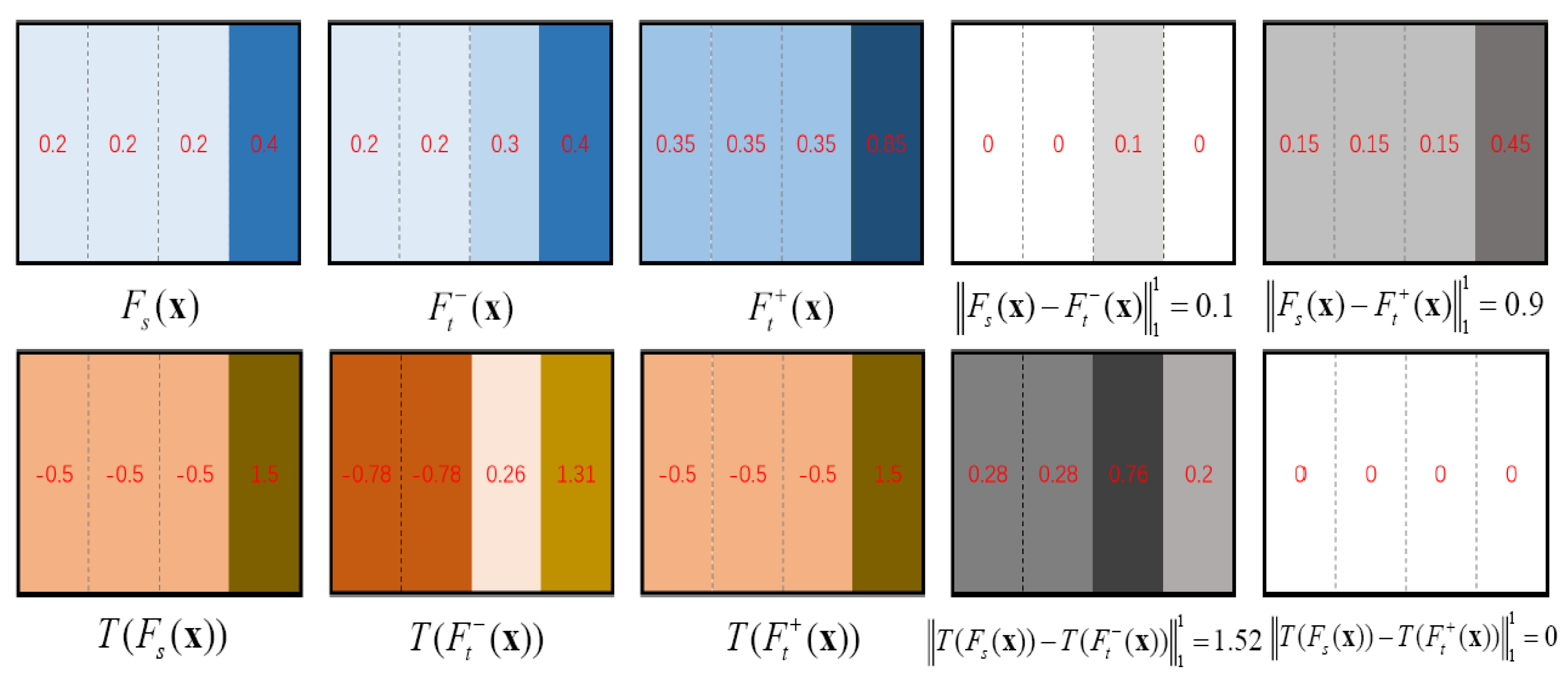
To show the strong discriminability of the matching cost using a correlation coefficient, we directly compare it with the previous matching cost using cross-correlation:

$${\mathrm{C}}_{\mathrm{p}}\left({\mathrm{F}}_{\mathrm{s}}\left(\mathrm{x}\right),{\mathrm{F}}_{\mathrm{t}}\left(\mathrm{y}\right)\right)=\frac{1}{\mathrm{D}}{\displaystyle \sum }_{\mathrm{h}=1}^{\mathrm{D}}{\mathrm{F}}_{\mathrm{s}}^{\mathrm{h}}\left(\mathrm{x}\right)·{\mathrm{F}}_{\mathrm{t}}^{\mathrm{h}}\left(\mathrm{y}\right)$$

(6)

Figure 2 provides a visual comparison to show the discriminability of ${\mathrm{C}}_{\mathrm{p}}\left({\mathrm{F}}_{\mathrm{s}}\left(\mathrm{x}\right),{\mathrm{F}}_{\mathrm{t}}\left(\mathrm{y}\right)\right)$ and $\mathrm{C}\left({\mathrm{F}}_{\mathrm{s}}\left(\mathrm{x}\right),{\mathrm{F}}_{\mathrm{t}}\left(\mathrm{y}\right)\right)$, where ${\mathrm{F}}_{\mathrm{t}}^{+}\left(\mathrm{y}\right)$ and ${\mathrm{F}}_{\mathrm{t}}^{-}\left(\mathrm{y}\right)$ are the matched and unmatched target features for the source feature ${\mathrm{F}}_{\mathrm{s}}\left(\mathrm{x}\right)$, respectively. ${\mathrm{F}}_{\mathrm{s}}\left(\mathrm{x}\right)$ and ${\mathrm{F}}_{\mathrm{t}}^{+}\left(\mathrm{y}\right)$ are the matched feature pair with the same gradients but a large difference in appearance, and ${\mathrm{F}}_{\mathrm{s}}\left(\mathrm{x}\right)$ and ${\mathrm{F}}_{\mathrm{t}}^{-}\left(\mathrm{y}\right)$ are the unmatched feature pair with similar appearances. This shows that when a source feature vector ${\mathrm{F}}_{\mathrm{s}}\left(\mathrm{x}\right)$ and a target feature vector ${\mathrm{F}}_{\mathrm{t}}^{+}\left(\mathrm{y}\right)$ have the similar gradients, even with different feature values, their feature transformations $T\left({\mathrm{F}}_{\mathrm{s}}\left(\mathrm{x}\right)\right)=\frac{{\mathrm{F}}_{\mathrm{s}}\left(\mathrm{x}\right)-{\mathsf{\mu }}_{\mathrm{s}}\left(\mathrm{x}\right)}{{\mathsf{\sigma }}_{\mathrm{s}}\left(\mathrm{x}\right)}$ and $\mathrm{T}\left({\mathrm{F}}_{\mathrm{t}}^{+}\left(\mathrm{x}\right)\right)=\frac{{\mathrm{F}}_{\mathrm{t}}^{+}\left(\mathrm{x}\right)-{\mathsf{\mu }}_{\mathrm{t}}^{+}\left(\mathrm{x}\right)}{{\mathsf{\sigma }}_{\mathrm{t}}^{+}\left(\mathrm{x}\right)}$ still have the same feature values, that is $\Vert T\left({\mathrm{F}}_{\mathrm{s}}\left(\mathrm{x}\right)\right)-\mathrm{T}\left({\mathrm{F}}_{\mathrm{t}}^{+}\left(\mathrm{x}\right)\right)\Vert {}_1{}^1=0$, and the correlation coefficient between ${\mathrm{F}}_{\mathrm{s}}\left(\mathrm{x}\right)$ and ${\mathrm{F}}_{\mathrm{t}}^{+}\left(\mathrm{y}\right)$ has a relatively large value. Otherwise, even if a source feature vector ${\mathrm{F}}_{\mathrm{s}}\left(\mathrm{x}\right)$ and a target feature vector ${\mathrm{F}}_{\mathrm{t}}^{-}\left(\mathrm{y}\right)$ have a similar appearance or similar feature values, but with different gradients, their feature transformations $T\left({\mathrm{F}}_{\mathrm{s}}\left(\mathrm{x}\right)\right)=\frac{{\mathrm{F}}_{\mathrm{s}}\left(\mathrm{x}\right)-{\mathsf{\mu }}_{\mathrm{s}}\left(\mathrm{x}\right)}{{\mathsf{\sigma }}_{\mathrm{s}}\left(\mathrm{x}\right)}$ and $\mathrm{T}\left({\mathrm{F}}_{\mathrm{t}}^{-}\left(\mathrm{x}\right)\right)=\frac{{\mathrm{F}}_{\mathrm{t}}^{-}\left(\mathrm{x}\right)-{\mathsf{\mu }}_{\mathrm{t}}^{-}\left(\mathrm{x}\right)}{{\mathsf{\sigma }}_{\mathrm{t}}^{-}\left(\mathrm{x}\right)}$ are still different, that is $\Vert T\left({\mathrm{F}}_{\mathrm{s}}\left(\mathrm{x}\right)\right)-\mathrm{T}\left({\mathrm{F}}_{\mathrm{t}}^{-}\left(\mathrm{x}\right)\right)\Vert {}_1{}^1=1.52$, and the correlation coefficient between ${\mathrm{F}}_{\mathrm{s}}\left(\mathrm{x}\right)$ and ${\mathrm{F}}_{\mathrm{t}}^{-}\left(\mathrm{y}\right)$ has a relatively small value.

The above description reveals the reason why the correlation coefficient is used as the matching cost: it can enhance the discriminability of the feature matching. However, ${\mathrm{C}}_{\mathrm{p}}$ directly takes the cross correlation as the matching cost, which will fluctuate greatly when the feature values change drastically due to the influence of the changes in the fluid shapes and illuminations. The value of its matching cost does not reflect the matching degree between any two feature vectors.

3.4. Multi-Scale Cost Volume

For each iteration, the multi-scale cost volume is constructed by performing a multi-scale search from the correlation pyramid with the initial matches, which are the predicted matches for the sparse seeds in the last iteration. For the first iteration, the initial matches are set to zero. After obtaining the initial match $\mathrm{f}\left({\mathrm{s}}_{\mathrm{x}}\right)$ for the current seed ${\mathrm{s}}_{\mathrm{x}}$ in ${\mathrm{I}}_1$, we assume the corresponding matching position in ${\mathrm{I}}_2$ is given by $\mathrm{M}\left(\mathrm{p}\left({\mathrm{s}}_{\mathrm{x}}\right)\right)=\mathrm{p}\left({\mathrm{s}}_{\mathrm{x}}\right)+\mathrm{f}\left({\mathrm{s}}_{\mathrm{x}}\right)$. Here, we define a search space: $\left\{\mathrm{M}\left(\mathrm{p}\left({\mathrm{s}}_{\mathrm{x}}\right)\right)+\mathrm{r}|\mathrm{r}\in {\mathbb{Z}}^2,{\mathrm{r}}_1\le \mathrm{r}\right\}$, which is centered at $\mathrm{M}\left(\mathrm{p}\left({\mathrm{s}}_{\mathrm{x}}\right)\right)$ and has a search radius of $r$ in both horizontal and vertical directions. We look up the matching costs from the multi-scale correlation volume by indexing a set of integer coordinates in the search space. Specifically, the set of the searched matching costs at the level $k$ of the correlation pyramid is given by:

$${\mathrm{C}}_{\mathrm{S}}^{\left(\mathrm{k}\right)}=\left\{{\mathrm{C}}^{\left(\mathrm{k}\right)}\left({\mathrm{F}}_{\mathrm{s}}\left(\mathrm{p}\left({\mathrm{s}}_{\mathrm{x}}\right)\right),{\mathrm{F}}_{\mathrm{t}}\left(\raisebox{1ex}{$\mathrm{M}\left(\mathrm{p}\left({\mathrm{s}}_{\mathrm{x}}\right)\right)$}\!\left/ \!\raisebox{-1ex}{$2^{\left(\mathrm{k}\right)}$}\right.+\mathrm{r}\right)\right)|\mathrm{r}\in {\mathbb{Z}}^2,{\Vert \mathrm{r}\Vert }_1\le \mathrm{r}\right\}$$

(7)

where ${\mathrm{C}}_{\mathrm{S}}^{\left(\mathrm{k}\right)}$ is a correlation feature block, we perform lookups on all the levels of the correlation pyramid and search for the matching costs with a constant radius $\mathrm{r}$ at each level, and the multi-scale cost volume is constructed by the concatenation of the correlation feature block ${\mathrm{C}}_{\mathrm{S}}^{\left(\mathrm{k}\right)}\left(\mathrm{k}=0,1,2,3\right)$ at different levels.

Now, we discuss the advantages of the multi-scale cost volume using a constant search radius. A constant radius across levels of the correlation pyramid means a larger coverage when the radius at the higher level is mapped to the lower level. For instance, when the level of the correlation pyramid $\mathrm{L}=4$, if a constant radius $\mathrm{r}=4$ at the coarsest level, it corresponds to a relatively large radius of $2^{\mathrm{L}-1}·\mathrm{r}=32$ at the finest level. If the interval of the sparse seeds is set to $\mathrm{n}=3$, it has a larger radius of $2^{\mathrm{L}-1}·\mathrm{r}·2^{\mathrm{n}}=256$ at the full resolution of image. Finally, the matching costs searched from different levels are then concatenated into a single feature block, named the multi-scale cost volume. Through a multiscale search strategy, the multi-scale cost volume contains global and local motion information, which can avoid the corresponding matches falling into the local minimum and also provides a guarantee for the recovery of the local small-scale motion structures.

3.5. CNN-Based Update Module

In this section, we introduce a CNN-based update module with a recurrent neural network, which is a gated activation unit based on the GRU cell. As in [11], it takes a context feature, the current matches, the multi-scale cost volume, and a hidden state as input and outputs the updated matches and an updated hidden state. Specifically, its update operator is given as follows:

$$\begin{gathered} {\mathrm{z}}_{\mathrm{t}}^{\mathrm{d}}=\mathsf{\sigma }\left({\mathrm{Conv}}_{\mathrm{z}\left({\mathrm{W}}_{\mathrm{z}}^{\mathrm{d}},\left[{\mathrm{h}}_{\mathrm{t}-1}^{\mathrm{d}},{\mathrm{x}}_{\mathrm{t}}^{\mathrm{d}}\right]\right)}\right) \\ {\mathrm{r}}_{\mathrm{t}}^{\mathrm{d}}=\mathsf{\sigma }\left({\mathrm{Conv}}_{\mathrm{r}\left({\mathrm{W}}_{\mathrm{r}}^{\mathrm{d}},\left[{\mathrm{h}}_{\mathrm{t}-1}^{\mathrm{d}},{\mathrm{x}}_{\mathrm{t}}^{\mathrm{d}}\right]\right)}\right) \\ {\tilde{\mathrm{h}}}_{\mathrm{t}}^{\mathrm{d}}=\tan \mathrm{h}\left({\mathrm{Conv}}_{\mathrm{h}\left({\mathrm{W}}_{\mathrm{h}}^{\mathrm{d}},\left[{\mathrm{r}}_{\mathrm{t}}^{\mathrm{d}}{\ast \mathrm{h}}_{\mathrm{t}-1}^{\mathrm{d}},{\mathrm{x}}_{\mathrm{t}}^{\mathrm{d}}\right]\right)}\right) \\ {\mathrm{h}}_{\mathrm{t}}^{\mathrm{d}}=\left(1-{\mathrm{z}}_{\mathrm{t}}^{\mathrm{d}}\right)\ast {\mathrm{h}}_{\mathrm{t}-1}^{\mathrm{d}}+{\mathrm{z}}_{\mathrm{t}}^{\mathrm{d}}\ast {\tilde{\mathrm{h}}}_{\mathrm{t}}^{\mathrm{d}} \\ {\mathrm{y}}_{\mathrm{t}}^{\mathrm{d}}=\mathsf{\sigma }\left(\mathrm{Conv}\_\mathrm{y}\left({\mathrm{w}}_{\mathrm{y}}^{\mathrm{d}},{\mathrm{h}}_{\mathrm{t}}^{\mathrm{d}}\right)\right) \end{gathered}$$

(8)

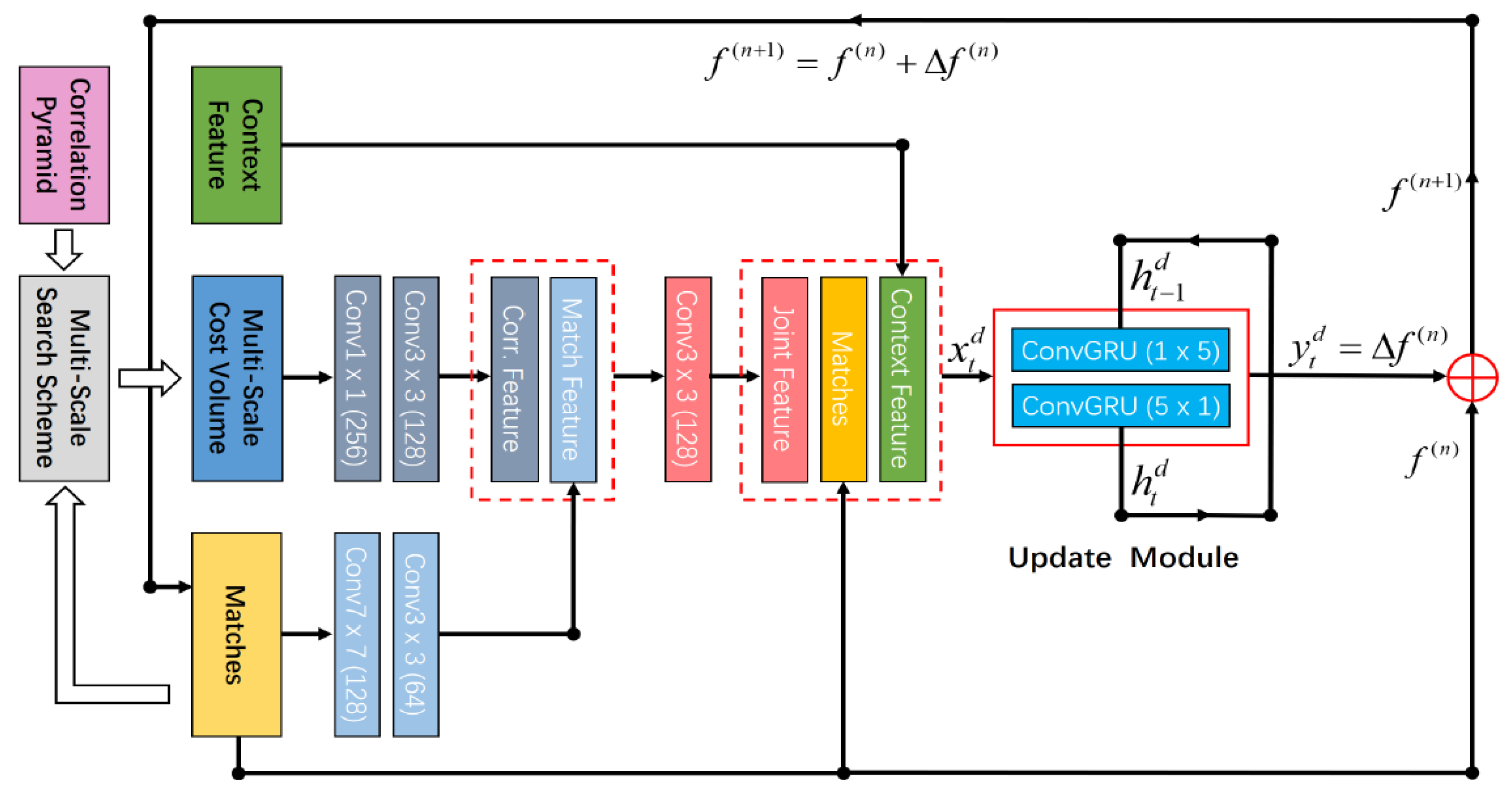
where ${\mathrm{x}}_{\mathrm{t}}^{\mathrm{d}}$ is an input feature map, which is taken as the concatenation of the context feature, the current matches, and the joint feature that combines both the feature of the searched multi-scale cost volume and the feature of the current matches. Specifically, this is given in Figure 3. We initialize the matches ${\mathrm{f}}^{\left(0\right)}$ of these sparse seeds to zero everywhere before the iteration. Given the current matches ${\mathrm{f}}^{\left(\mathrm{k}\right)}$, we retrieve the multiscale const volume from the correlation pyramid via a multi-scale search scheme. The searched multi-scale cost volume is then processed by two convolutional layers to generate the correlation feature, and the match feature is extracted from the current matches with two convolutional layers. The joint feature is extracted from the concatenation of both the correlation feature and the match feature using a convolutional layer. The output ${\mathrm{y}}_{\mathrm{t}}^{\mathrm{d}}$ is a predicted match offset ∆${\mathrm{f}}^{\left(\mathrm{k}\right)}$, which is generated using two convolution layers for the output hidden state ${\mathrm{h}}_{\mathrm{t}}^{\mathrm{d}}$ from the GRU. The predicted matches are updated by ${\mathrm{f}}^{\left(\mathrm{k}+1\right)}={\mathrm{f}}^{\left(\mathrm{k}\right)}$+∆${\mathrm{f}}^{\left(\mathrm{k}\right)}$, which is the sparse matches and $\raisebox{1ex}{$1$}\!\left/ \!\raisebox{-1ex}{$2^n$}\right.$ the resolution of the original input image. The CNN-based updated module contains two conGRU unit: one with a $1\times 5$ convolution and one with a $5\times 1$ convolution.

3.6. CNN-Based Interpolation

Since the predicted matches are sparse and $\raisebox{1ex}{$1$}\!\left/ \!\raisebox{-1ex}{$2^n$}\right.$ the resolution of the original input image, the sparse matches are upsampled to the full resolution by a CNN-based interpolation [11], which uses two convolutional layers for the output hidden state $h_t^d$ to predict a mask of size $\raisebox{1ex}{$\mathrm{H}$}\!\left/ \!\raisebox{-1ex}{$2^{\mathrm{n}}$}\right.\times \raisebox{1ex}{$\mathrm{W}$}\!\left/ \!\raisebox{-1ex}{$2^{\mathrm{n}}$}\right.\times \left(64\times 9\right)$ and perform softmax over the weights of the nine neighbors. The high-resolution flow field is computed by taking a weighted combination of the nine coarse resolution neighbors using the mask predicted by the network. During training and evaluation, the predicted matches $f$ are upsampled to the full resolution $F$, which is used to match the resolution of the ground truth.

As in [11], the loss function is defined as:

$$\xi ={\displaystyle \sum }_{i=1}^{N-1}{\lambda }^{N-i}·\Vert F_i^h-F_{gt}\Vert {}_1$$

(9)

where $F_{\mathrm{gt}}$ is the ground truth, and $N$ is the number of the iteration. $F_i^h$ is a predicted flow field in the $\mathrm{i}$th iteration, and ${\lambda }^{N-i}$ is the weight for the ${\mathrm{L}}_1$ distance between the predicted flow field $F_i^h$ and the ground truth $F_{gt}$. The loss function considers the predicted flow field in each iteration, and the weight ${\lambda }^{N-i}$ exponentially increases as the number of iterations increases.

4. Experiments

4.1. Datasets and Evaluation Metrics

In this section, we perform our method on the public fluid datasets and the real-world remote sensing images: (1) A 2D turbulent flow from the second set of fluid mechanics image sequences; (2) A surface quasi-geostrophic (SQG) model of sea flow; (3) Jupiter’s White Ovals.

(1) The 2D DNS-turbulent flow [33]: DNS-turbulent flow is a homogeneous, isotropic, and incompressible turbulent flow, which is generated by direct numerical simulation of the Navier–Stokes equations. This dataset contains typical difficulties for PIV measurement methods, such as high velocity gradients and small-scale vortices, and it has become a benchmark for evaluating the fluid motion estimators.

(2) The SQG flow [34]: SQG flow is geophysical flow under location uncertainty. It is created from a surface quasi-geostrophic model of sea flow and contains a great many small-scale vortices.

(3) Jupiter’s White Ovals [35]: Jupiter’s White Ovals are distinct storms in Jupiter’s atmosphere, and the remote sensing images are taken by the NASA’s Galileo Solid State Imaging system. It is key to understand the physical mechanisms of their forming and sustaining by extracting the velocity field of Jupiter’s White Ovals by their images. Therefore, it is of great significance to analyze the motion of Jupiter’s atmosphere based on the observed data.

The most commonly used measure of performance for fluid flows is the average endpoint error (AEE) [36], which is given by:

$$\mathrm{AEE}=\frac{1}{N}{\displaystyle \sum }_{i=1}^N\sqrt{\left[{\left(u_i-u_{ti}\right)}^2+{\left(v_i-v_{ti}\right)}^2\right]}$$

(10)

where $u_i$ and $v_i$ denote the horizontal and vertical components of the estimated flow vector at the position $i$, and $u_{ti}$ and $v_{ti}$ denote the horizontal and vertical components of the ground-truth flow at the position $i$. $N$ is the number of pixels in the image.

4.2. Parameter Detail

We perform our method with an intel (R) core (TM) i9-9900k CPU @3.6GHz. Our network parameter model is trained using the particle image sequences (DNS-turbulent [33], SQG [34], and JHTDB [37]) from PIV-dataset [10]. The batch size is set to 8, and the parameter $\lambda =0.8$. For the AdamW optimizer, the weight decay is set to 0.0001, and the learning rate is set to 0.00025. Our method runs about 0.36 s for a particle image pair with a resolution of $256\times 256$ pixels using Pytorch on a NVIDIA GeForce RTX 2070 GPU.

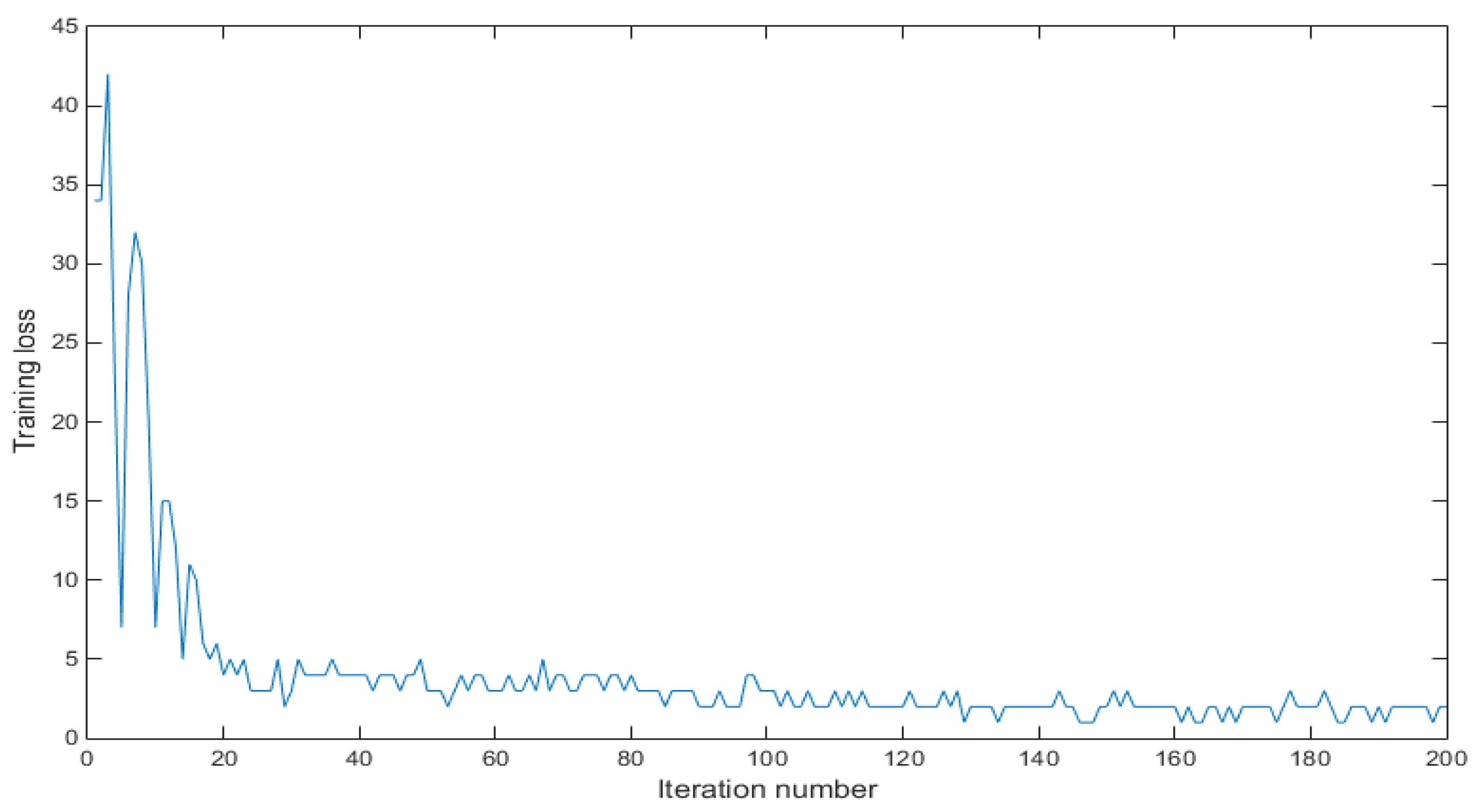
To monitor the training progress, we provide the curve of training process in Figure 4, which plots the training loss for each iteration.

4.3. Main Results and Analysis

4.3.1. DNS-Turbulent Flow

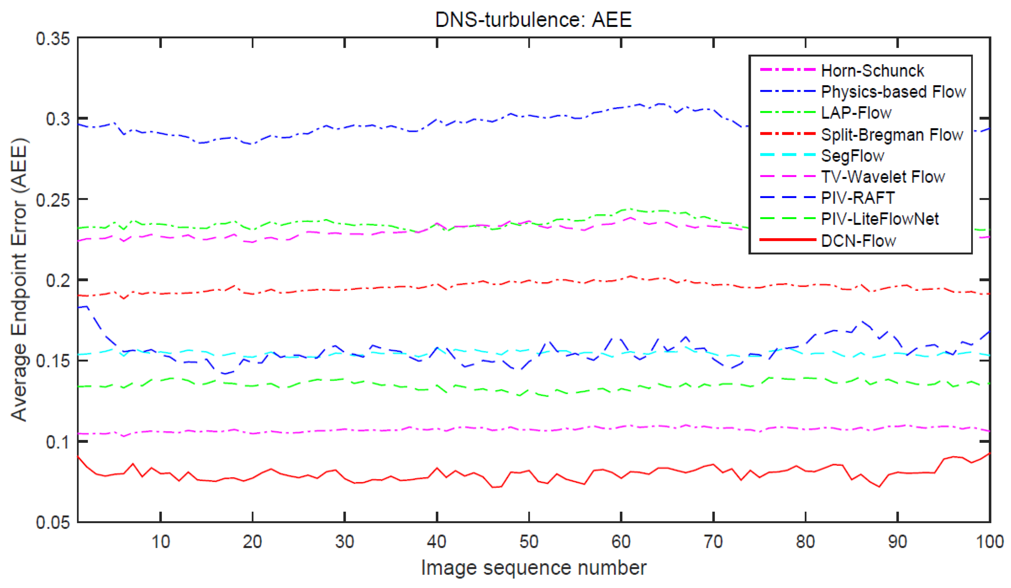
We compare our method with the current state-of-the art motion estimators. Figure 5 shows the curves of AEE (average endpoint error) for different optical flow methods, where we perform the experiments on the 100 successive images with the size of 256 × 256 pixels from 2D DNS-turbulent flow. The evaluation results in Figure 6 show that our method achieves better performance than the traditional motion estimators (such as Physics Flow [38] and TV-Wavelet Flow [39]) and CNN-based motion estimators (PIV-LiteFlowNet [10] and PIV-RAFT [11]). It has a significant improvement in accuracy, and the main reason for this is that our method uses correlation coefficients as the matching costs, which can overcome the feature distortions caused by the changes of fluid shapes and illuminations and improve the accuracy of motion estimation by enhancing the discrimination of the feature matching.

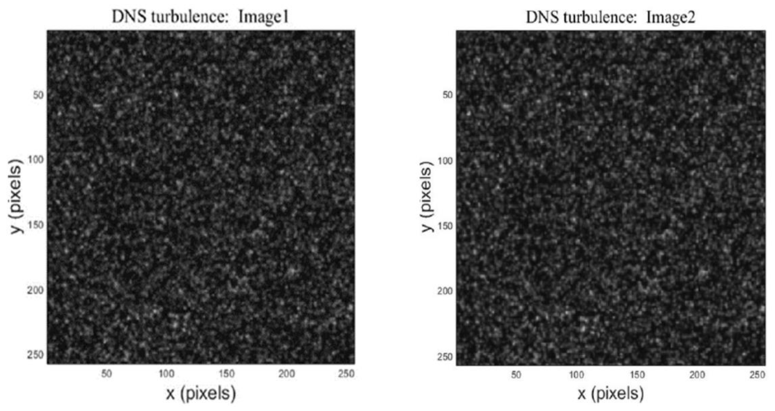
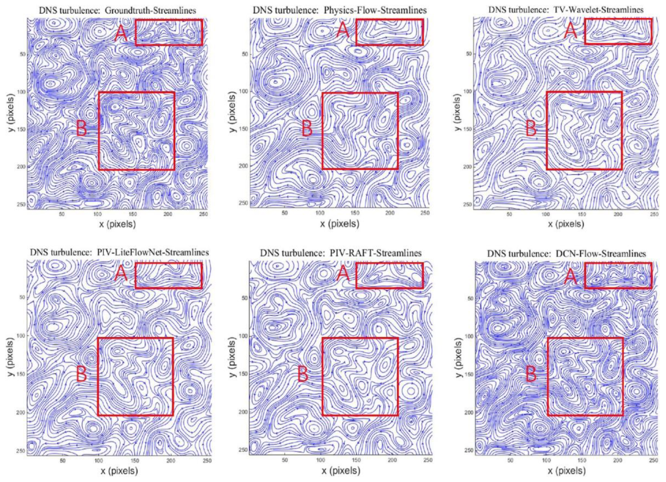
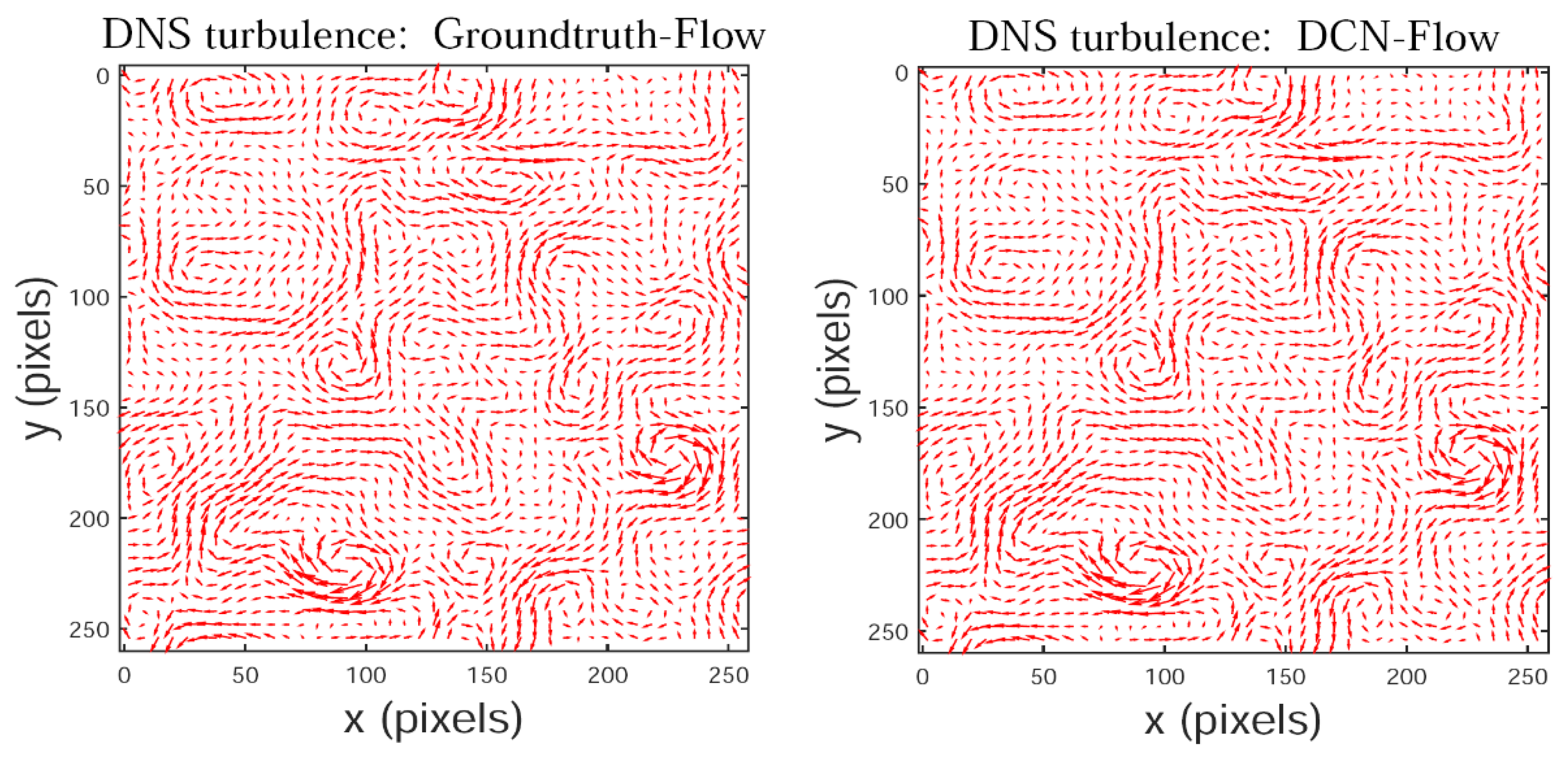
Figure 6 shows an image pair from DNS-turbulent flow, and the corresponding streamlines of different motion estimators are shown in Figure 7. The streamlines allow us to better observe the vortices in complex fluid flows, and the streamlines in Figure 7 show that our method significantly outperforms the current motion estimators in recovering small-scale vortices. The main reason is that the multi-scale cost volume is used for our method to recover the moving structures with both large and small displacements, especially to capture the motion of small fast-moving objects, such as some important small-scale vortices in complex fluid flows. Figure 8 shows that the visual flow vectors estimated by our method are very similar to the ground-truth flow vectors.

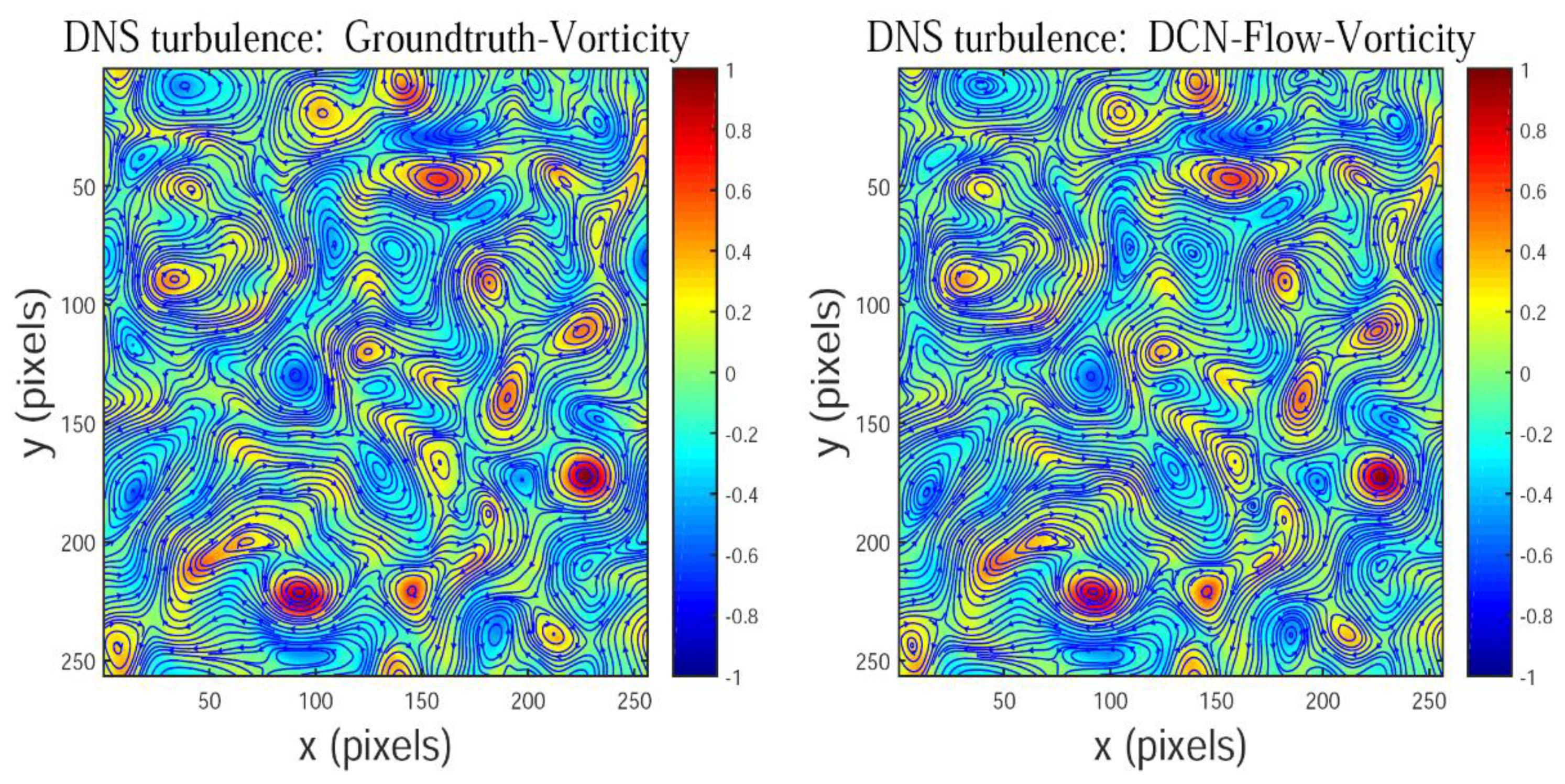
In this paper, to facilitate observation and analysis, the color-coded vorticity field is produced by performing a Gaussian filtering for vorticity field normalized by its maximum values. The red and blue colors represent positive and negative curls, respectively. Figure 9 shows that the vorticity predicted by our method is also consistent with the corresponding ground truth, and simultaneously the designed CNN-based motion estimator can successfully locate the centers of these vortices, which are marked in a red or blue color.

4.3.2. SQG Flow

Figure 10 provides the curves of AEE (average endpoint error) for different motion estimators, where we perform experiments on the 50 successive images from SQG flow. The evaluation results in Figure 10 show that our method significantly outperforms other motion estimators. The main reason is that our method uses correlation coefficients as the matching costs, which can improve the accuracy of motion estimation by enhancing the discrimination of the feature matching and overcoming the feature distortions caused by the changes of fluid shapes and illuminations.

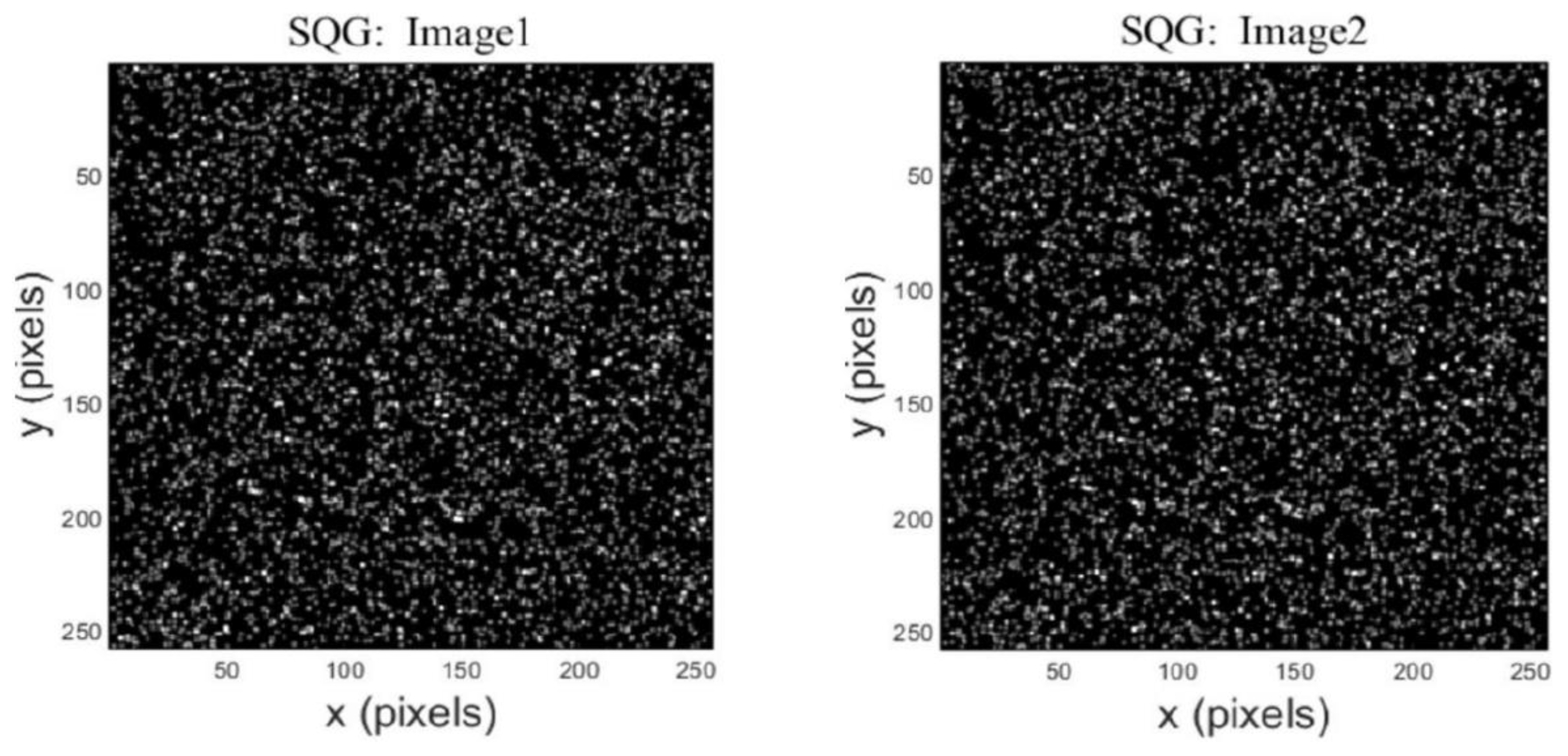
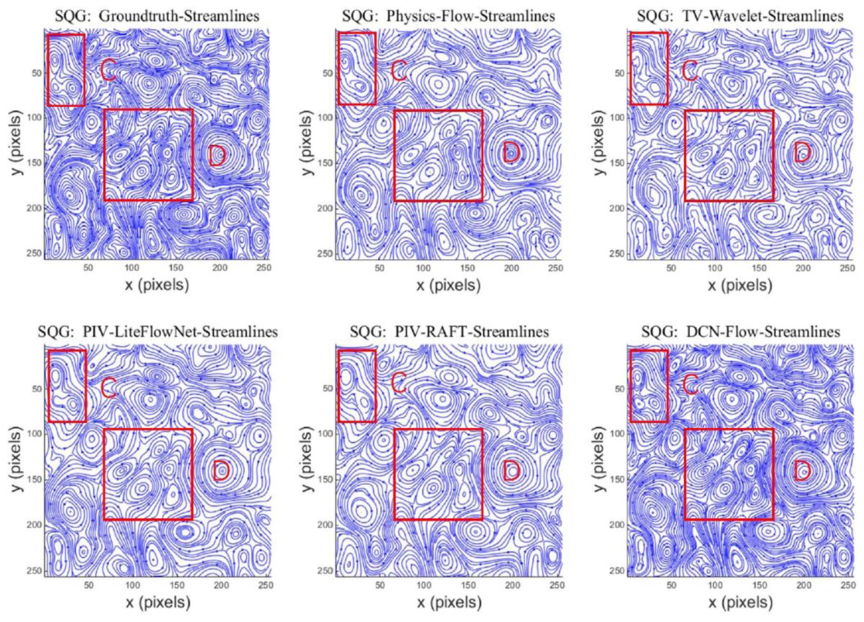
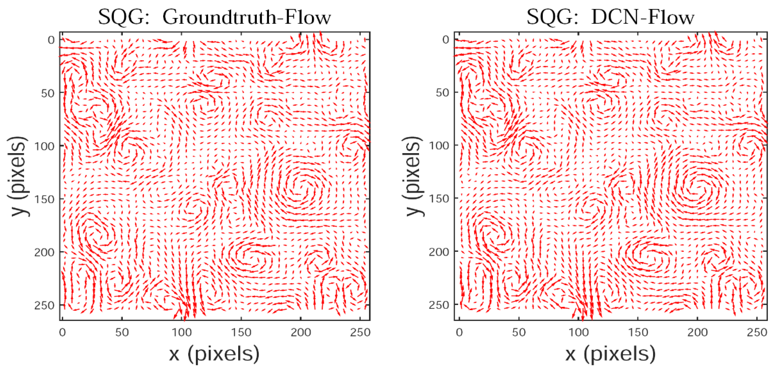
Figure 11 shows an image pair from SQG flow, which contains many small-scale vortices. The streamlines in Figure 12 show that our method performs better than other motion estimators in capturing small-scale vortices, and the estimated flow vectors of our method in Figure 13 are very similar to the ground-truth flow vectors. At the same time, Figure 14 shows that our method successfully locates the centers of these vortices, which are color-coded in red or blue. The main reason for this is that our method uses the multi-scale cost volume that contains both global and local motion information, so it can recover the moving structures with both large and small displacements, especially capture the motion of small fast-moving objects, such as important small-scale vortices in complex fluid flows.

4.3.3. Evaluation on the Fluid Datasets

The evaluation results of different motion estimators on the public fluid datasets are shown in

Table 1. Evaluation results of different motion estimators on the public fluid datasets.

Different Motion Estimators	DNS-Turbulence (AEE)	SQG (AEE)
Horn–Schunck [8]	0.107	0.329
Physics-Flow [38]	0.296	0.483
LAP-Flow [40]	0.234	0.357
Split-Bregman Flow [41]	0.195	0.320
SegFlow [42]	0.154	0.232
Translation-Flow [43]	0.110	0.259
Curl-Flow [43]	0.122	0.311
Divergence-Flow [43]	0.133	0.325
TV-Wavelet Flow [39]	0.230	0.371
PWC-Net [23]	0.831	1.126
RAFT [11]	0.920	1.334
PIV-RAFT [11]	0.156	0.294
PIV-LiteFlowNet [10]	0.135	0.206
DCN-Flow	0.080	0.148

, where PWC-Net [23] and RAFT [11] use the original pre-trained models. Based on the original pretrained model of RAFT [11], PIV-RAFT was trained with the particle image pairs from a 2D turbulent flow [33], SQG [34], and JHTDB [37]. PIV-LiteFlowNet [10] was trained with the particle image pairs from PIV dataset. The evaluation results show that our method (DCN-Flow) significantly outperforms the current motion estimators in predicting complex fluid flows.

4.3.4. Jupiter’s White Ovals

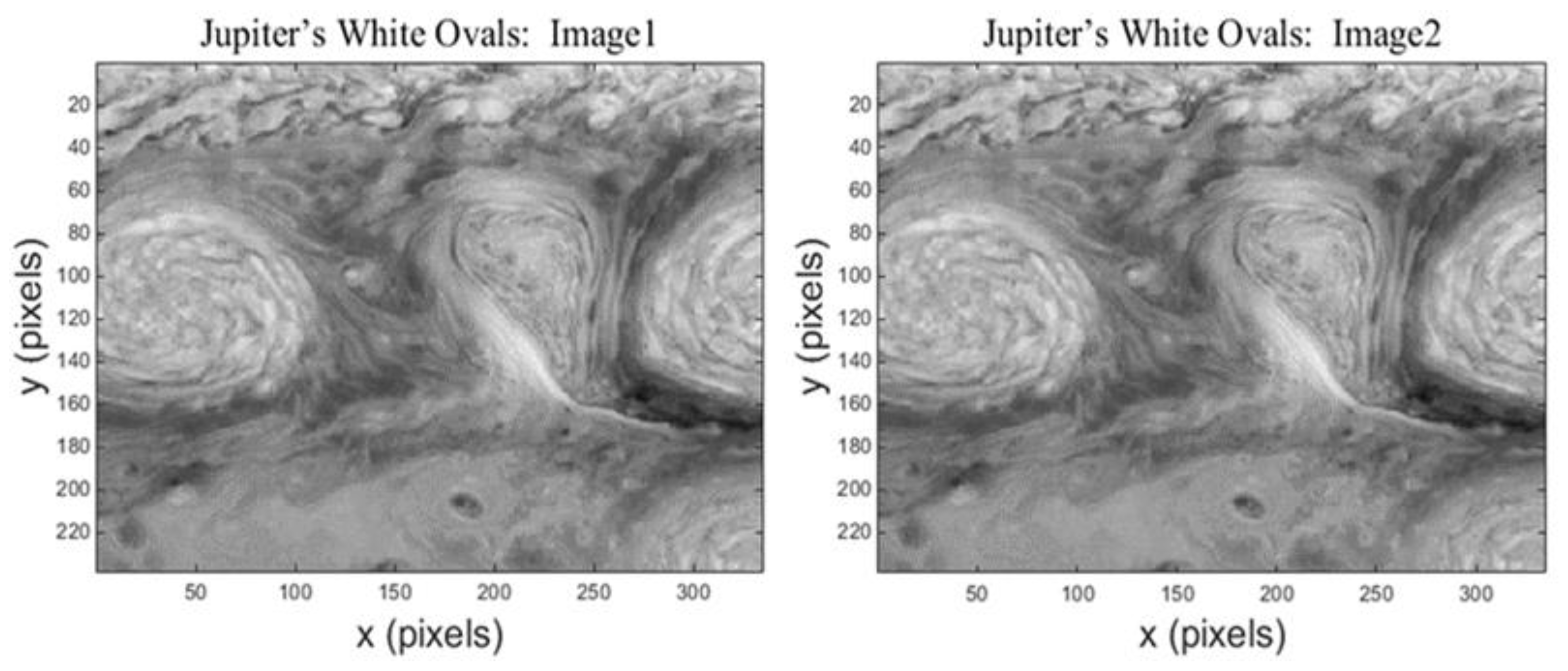
Figure 15 shows two successive images of Jupiter’s White Ovals, which were taken by NASA’s Galileo Solid State Imaging system. The illumination from the sun was considerably changed in a local and non-uniform fashion. To improve the accuracy of the predicted optical flow field by our method on the real-world image sequences, we train our network on FlyingChairs [21], FlyingThings [44], and MPI-Sintel training datasets [45].

The predicted flow field by our method for Jupiter’s White Ovals is shown in Figure 16. There exist three large vortices in Jupiter’s atmosphere, which correspond to Jupiter’s three white spots. The vortex in the middle of the image is balloon-shaped, and its corresponding cyclone rotates clockwise. The two vortices on both sides of the image are elliptical, and their corresponding cyclones rotate counterclockwise. The streamlines of the predicted flow field in Figure 17 show that our method successfully captured the storms in Jupiter’s White Ovals, including some important small-scale vortices.

4.3.5. Evaluation on Other Image Sequences

We also evaluate our method on other image sequences, such as video images from MPI-Sintel dataset [45], which provides naturalistic video sequences that are challenging for current methods. It is designed to encourage research on long-range motion, motion blur, multi-frame analysis, and non-rigid motion.

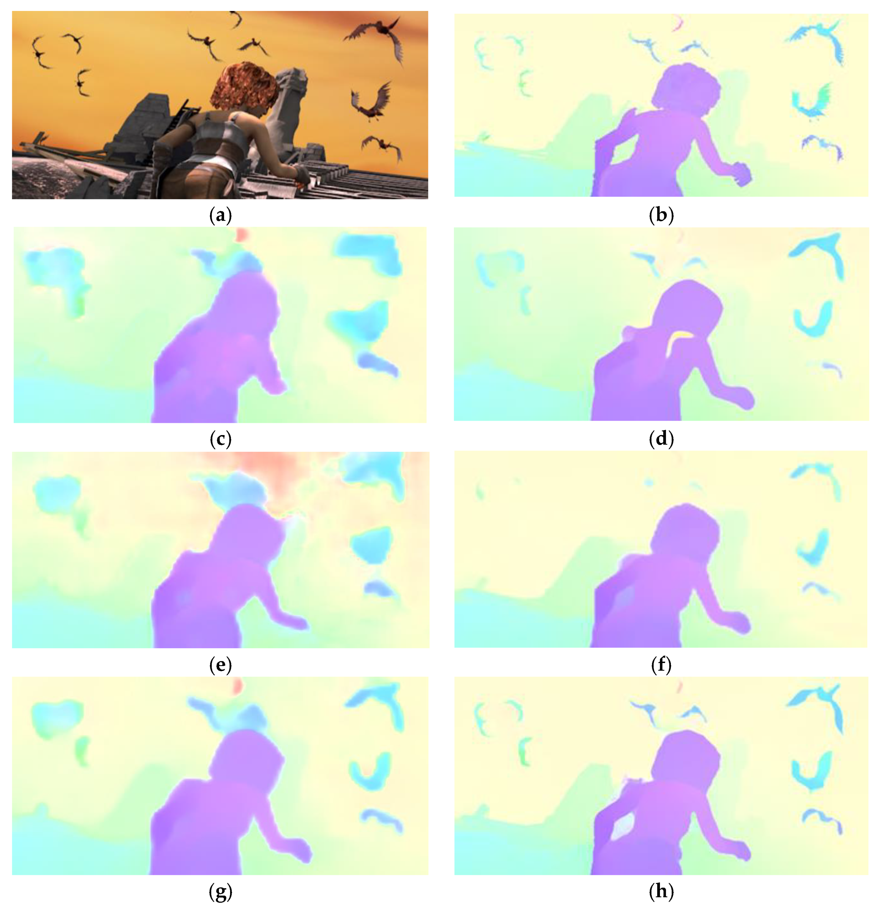
The evaluation results in

Table 2. Evaluation results of different motion estimators on the MPI-Sintel test dataset.

Different Motion Estimators	Final (EPE all) 1	Clean (EPE all) 1
GMA [26]	2.470	1.388
RAFT [11]	2.855	1.609
DCN-Flow	3.186	2.326
Flow1D [46]	3.806	2.238
MaskFlownet [47]	4.172	2.521
LiteFlowNet3 [48]	4.448	2.994
PWC-Net [23]	5.042	4.386
LiteFlowNet [24]	5.381	4.539
ARFlow [25]	5.889	4.782
Flownet2 [22]	6.016	3.959
Horn–Schunck [8]	9.610	8.739

¹ EPE all: endpoint error over the complete frames.

show that our method (DCN-Flow) achieves a high ranking on the MPI-Sintel test dataset. It performs better than some current CNN-based motion estimators [22,23,24,25,46,47,48]. Figure 18 shows visual comparison of optical flow fields estimated by different motion estimators. It shows that our method achieves better performance than the current CNN-based motion estimators [22,23,25,47,48] in preserving sharp flow edges and recovering important motion details.

5. Conclusions

In this paper, we introduce a novel CNN-based motion estimator, and it uses correlation coefficients as the matching costs, which can improve the accuracy of motion estimation by enhancing the discrimination of the feature matching and overcoming the feature distortions caused by the changes of fluid shapes and illuminations. Since the searched multi-scale cost volume contains global and local motion information, it can recover both large and small displacements very well, especially capture small-scale motion structures. In the future, we will improve the accuracy of fluid motion estimation by designing more advanced CNN-based motion estimators, which consider the physical laws of fluid flow evolution, such as the Helmholtz decomposition of vector fields, Navier–Stokes equations, etc.

References

1. Heitz, D.; Héas, P.; Mémin, E.; Carlier, J. Dynamic consistent correlation-variational approach for robust optical flow estimation. Exp. Fluids 2008, 45, 595–608. [Google Scholar] [CrossRef]
2. Astarita, T. Analysis of velocity interpolation schemes for image deformation methods in PIV. Exp. Fluids 2008, 45, 257–266. [Google Scholar] [CrossRef]
3. Astarita, T. Adaptive space resolution for PIV. Exp. Fluids 2009, 46, 1115–1123. [Google Scholar] [CrossRef]
4. Becker, F.; Wieneke, B.; Petra, S.; Schröder, A.; Schnörr, C. Variational Adaptive Correlation Method for Flow Estimation. IEEE Trans. Image Process. 2011, 21, 3053–3065. [Google Scholar] [CrossRef]
5. Theunissen, R.; Scarano, F.; Riethmuller, M.L. An adaptive sampling and windowing interrogation method in PIV. Meas. Sci. Technol. 2006, 18, 275–287. [Google Scholar] [CrossRef]
6. Theunissen, R.; Scarano, F.; Riethmuller, M.L. Spatially adaptive PIV interrogation based on data ensemble. Exp. Fluids 2009, 48, 875–887. [Google Scholar] [CrossRef]
7. Yu, K.; Xu, J. Adaptive PIV algorithm based on seeding density and velocity information. Flow Meas. Instrum. 2016, 51, 21–29. [Google Scholar] [CrossRef]
8. Horn, B.K.P.; Schunck, B.G. Determining optical flow. Artif. Intell. 1981, 17, 185–203. [Google Scholar] [CrossRef] [Green Version]
9. Cai, S.; Liang, J.; Gao, Q.; Xu, C.; Wei, R. Particle Image Velocimetry Based on a Deep Learning Motion Estimator. IEEE Trans. Instrum. Meas. 2019, 69, 3538–3554. [Google Scholar] [CrossRef]
10. Cai, S.; Zhou, S.; Xu, C.; Gao, Q. Dense motion estimation of particle images via a convolutional neural network. Exp. Fluids 2019, 60, 73. [Google Scholar] [CrossRef]
11. Teed, Z.; Deng, J. RAFT: Recurrent All-Pairs Field Transforms for Optical Flow. In Proceedings of the European Conference on Computer Vision 2020, Glasgow, UK, 23–28 August 2020; pp. 402–419. [Google Scholar] [CrossRef]
12. Brox, T.; Bruhn, A.; Papenberg, N.; Weickert, J. High Accuracy Optical Flow Estimation Based on a Theory for Warping. In Proceedings of the European Conference on Computer Vision, Prague, Czech Republic, 11–14 May 2004; pp. 25–36. [Google Scholar]
13. Zach, C.; Pock, T.; Bischof, H. A duality based approach for real-time TV-L1 optical flow. In Proceedings of the 29th DAGM Symposium, Heidelberg, Germany, 12–14 September 2007; pp. 214–223. [Google Scholar]
14. Corpetti, T.; Memin, E.; Perez, P. Dense estimation of fluid flows. IEEE Trans. Pattern Anal. Mach. Intell. 2002, 24, 365–380. [Google Scholar] [CrossRef] [Green Version]
15. Zhou, L.; Kambhamettu, C.; Goldgof, D. Fluid structure and motion analysis from multi-spectrum 2D cloud image sequences. In Proceedings of the IEEE Conference on Computer Vision and Pattern Recognition 2000, Hilton Head, SC, USA, 13–15 June 2002; Volume 2, pp. 744–751. [Google Scholar] [CrossRef] [Green Version]
16. Sakaino, H. Optical flow estimation based on physical properties of waves. In Proceedings of the IEEE Conference on Computer Vision and Pattern Recognition, Anchorage, AK, USA, 23–28 June 2008; pp. 1–8. [Google Scholar]
17. Sakaino, H. Spatio-Temporal Image Pattern Prediction Method Based on a Physical Model with Time-Varying Optical Flow. IEEE Trans. Geosci. Remote Sens. 2012, 51, 3023–3036. [Google Scholar] [CrossRef]
18. Li, F.; Xu, L.; Guyenne, P.; Yu, J. Recovering fluid-type motions using Navier-Stokes potential flow. In Proceedings of the 2010 IEEE Computer Society Conference on Computer Vision and Pattern Recognition, San Francisco, CA, USA, 13–18 June 2010; pp. 2448–2455. [Google Scholar] [CrossRef]
19. Cuzol, A.; Hellier, P.; Memin, E. A low dimensional fluid motion estimator. Int. J. Comput. Vis. 2007, 75, 329–349. [Google Scholar] [CrossRef] [Green Version]
20. Ren, B.; He, W.; Li, C.-F.; Chen, X. Incompressibility Enforcement for Multiple-Fluid SPH Using Deformation Gradient. IEEE Trans. Vis. Comput. Graph. 2021, 28, 3417–3427. [Google Scholar] [CrossRef]
21. Dosovitskiy, A.; Fischer, P.; Ilg, E.; Hausser, P.; Hazirbas, C.; Golkov, V.; Van Der Smagt, P.; Cremers, D.; Brox, T. FlowNet: Learning Optical Flow with Convolutional Networks. In Proceedings of the 2015 IEEE International Conference on Computer Vision, Santiago, Chile, 7–13 December 2015; pp. 2758–2766. [Google Scholar]
22. Ilg, E.; Mayer, N.; Saikia, T.; Keuper, M.; Dosovitskiy, A.; Brox, T. Flownet 2.0: Evolution of optical flow estimation with deep networks. In Proceedings of the IEEE Conference on Computer Vision and Pattern Recognition, Honolulu, HI, USA, 21–26 July 2017; pp. 2462–2470. [Google Scholar]
23. Sun, D.; Yang, X.; Liu, M.; Kautz, J. PWC-Net: CNNs for optical flow using pyramid, warping, and cost volume. In Proceedings of the IEEE Conference on Computer Vision and Pattern Recognition, Salt Lake City, UT, USA, 18–22 June 2018. [Google Scholar]
24. Hui, T.W.; Tang, X.; Change, L.C. Liteflownet: A lightweight convolutional neural network for optical flow estimation. In Proceedings of the IEEE Conference on Computer Vision and Pattern Recognition, Salt Lake City, UT, USA, 18–22 June 2018; pp. 8981–8989. [Google Scholar]
25. Liu, L.; Zhang, J.; He, R.; Liu, Y.; Wang, Y.; Tai, Y.; Luo, D.; Wang, C.; Li, J.; Huang, F. Learning by Analogy: Reliable Supervision from Transformations for Unsupervised Optical Flow Estimation. In Proceedings of the IEEE/CVF Conference on Computer Vision and Pattern Recognition 2020, Seattle, WA, USA, 13–19 June 2020; pp. 6488–6497. [Google Scholar] [CrossRef]
26. Jiang, S.; Campbell, D.; Lu, Y.; Li, H.; Hartley, R. Learning to Estimate Hidden Motions with Global Motion Aggregation. In Proceedings of the IEEE/CVF International Conference on Computer Vision 2021, Montreal, QC, Canada, 10–17 October 2021; pp. 9752–9761. [Google Scholar] [CrossRef]
27. Masaki, M.; Kai, F.; Kai, Z.; Aditya, G.N.; Koji, F. Convolutional neural networks for fluid flow analysis: Toward effective metamodeling and low dimensionalization. Theor. Comput. Fluid Dyn. 2021, 35, 633–658. [Google Scholar]
28. Murata, T.; Fukami, K.; Fukagata, K. Nonlinear mode decomposition with convolutional neural networks for fluid dynamics. J. Fluid Mech. 2019, 882, A13. [Google Scholar] [CrossRef]
29. Nakamura, T.; Fukagata, K. Robust training approach of neural networks for fluid flow state estimations. Int. J. Heat Fluid Flow 2022, 96, 108997. [Google Scholar] [CrossRef]
30. Yu, C.; Luo, H.; Fan, Y.; Bi, X.; He, M. A Cascaded Convolutional Neural Network for Two-Phase Flow PIV of an Object Entering Water. IEEE Trans. Instrum. Meas. 2021, 71, 1–10. [Google Scholar] [CrossRef]
31. Liang, J.; Cai, S.; Xu, C.; Chen, T.; Chu, J. DeepPTV: Particle Tracking Velocimetry for Complex Flow Motion via Deep Neural Networks. IEEE Trans. Instrum. Meas. 2022, 71, 1–16. [Google Scholar] [CrossRef]
32. Guo, C.; Fan, Y.; Yu, C.; Han, Y.; Bi, X. Time-Resolved Particle Image Velocimetry Algorithm Based on Deep Learning. IEEE Trans. Instrum. Meas. 2022, 71, 1–13. [Google Scholar] [CrossRef]
33. Carlier, J. Second Set of Fluid Mechanics Image Sequences. European Project Fluid Image Analysis and Description (FLUID). 2005. Available online: http://www.fluid.irisa.fr (accessed on 1 June 2005).
34. Resseguier, V.; Memin, E.; Chapron, B. Geophysical flows under location uncertainty, Part II: Quasi-geostrophic models and efficient ensemble spreading. Geophys. Astrophys. Fluid Dyn. 2017, 111, 177–208. [Google Scholar] [CrossRef] [Green Version]
35. Vasavada, A.R.; Ingersoll, A.P.; Banfield, D.; Bell, M.; Gierasch, P.J. Galileo imaging of Jupiter’s atmosphere: The great red spot, equatorial region, and white ovals. Icarus 1998, 135, 265–275. [Google Scholar] [CrossRef]
36. Baker, S.; Scharstein, D.; Lewis, J.P.; Roth, S.; Black, M.J.; Szeliski, R. A Database and Evaluation Methodology for Optical Flow. Int. J. Comput. Vis. 2010, 92, 1–31. [Google Scholar] [CrossRef] [Green Version]
37. Li, Y.; Perlman, E.; Wan, M.; Yang, Y.; Meneveau, C.; Burns, R.; Chen, S.; Szalay, A.; Eyink, G. A public turbulence database cluster and applications to study Lagrangian evolution of velocity increments in turbulence. J. Turbul. 2008, 9, N31. [Google Scholar] [CrossRef] [Green Version]
38. Liu, T. OpenOpticalFlow: An Open Source Program for Extraction of Velocity Fields from Flow Visualization Images. J. Open Res. Softw. 2017, 5, 29. [Google Scholar] [CrossRef] [Green Version]
39. Chen, J.; Lai, J.; Cai, Z.; Xie, X.; Pan, Z. Optical Flow Estimation Based on the Frequency-Domain Regularization. IEEE Trans. Circuits Syst. Video Technol. 2021, 31, 217–230. [Google Scholar] [CrossRef]
40. Gilliam, C.; Blu, T. Local All-Pass Geometric Deformations. IEEE Trans. Image Process. 2017, 27, 1010–1025. [Google Scholar] [CrossRef]
41. Chen, J.; Cai, Z.; Lai, J.; Xie, X. Fast Optical Flow Estimation Based on the Split Bregman Method. IEEE Trans. Circuits Syst. Video Technol. 2018, 28, 664–678. [Google Scholar] [CrossRef]
42. Chen, J.; Cai, Z.; Lai, J.; Xie, X. Efficient Segmentation-Based PatchMatch for Large Displacement Optical Flow Estimation. IEEE Trans. Circuits Syst. Video Technol. 2019, 29, 3595–3607. [Google Scholar] [CrossRef]
43. Chen, J.; Cai, Z.; Lai, J.; Xie, X. A filtering-based framework for optical flow estimation. IEEE Trans. Circuits Syst. Video Technol. 2019, 29, 1350–1364. [Google Scholar] [CrossRef]
44. Mayer, N.; Ilg, E.; Hausser, P.; Fischer, P.; Cremers, D.; Dosovitskiy, A.; Brox, T. A large dataset to train convolutional networks for disparity, optical flow, and scene flow estimation. In Proceedings of the IEEE Conference on Computer Vision and Pattern Recognition, Las Vegas, NV, USA, 27–30 June 2016; pp. 4040–4048. [Google Scholar]
45. Butler, D.J.; Wulff, J.; Stanley, G.B.; Black, M.J. A naturalistic open source movie for optical flow evaluation. In European Conference on Computer Vision; Springer: Berlin/Heidelberg, Germany, 2012; pp. 611–625. [Google Scholar]
46. Xu, H.; Yang, J.; Cai, J.; Zhang, J.; Tong, X. High-Resolution Optical Flow from 1D Attention and Correlation. In Proceedings of the IEEE/CVF International Conference on Computer Vision 2021, Montreal, QC, Canada, 10–17 October 2021; pp. 10478–10487. [Google Scholar] [CrossRef]
47. Zhao, S.; Sheng, Y.; Dong, Y.; Chang, E.I.-C.; Xu, Y. MaskFlownet: Asymmetric Feature Matching with Learnable Occlusion Mask. In Proceedings of the IEEE/CVF Conference on Computer Vision and Pattern Recognition 2020, Seattle, WA, USA, 13–19 June 2020; pp. 6277–6286. [Google Scholar] [CrossRef]
48. Tak-Wai, H.; Chen, C.L. LiteFlowNet3: Resolving correspondence ambiguity for more accurate optical flow estimation. In Proceedings of the European Conference on Computer Vision, Glasgow, UK, 23–28 August 2020; pp. 169–184. [Google Scholar]
Figure 1. The structure of the feature extraction network.
Electronics 11 04159 g001
Figure 2. Visual comparison of the discriminability between C p ( F s ( x ) , F t ( y ) )   and C ( F s ( x ) , F t ( y ) ) .
Electronics 11 04159 g002
Figure 3. The overall structure of the proposed motion estimator using a deep convolution network.
Electronics 11 04159 g003
Figure 4. The curve of training process for our method (DCN-Flow).
Electronics 11 04159 g004
Figure 5. The curves of AEE (average endpoint error) for different optical flow methods (Horn–Schunck [8], Physics-based Flow [38], LAP-Flow [40], Split-Bregman Flow [41], SegFlow [42], TV-Wavelet Flow [39], PIV-RAFT [11], PIV-LiteFlowNet [10], DCN-Flow) on the 100 successive images of DNS-turbulent flow.
Electronics 11 04159 g005
Figure 6. An image pair from DNS-turbulent flow.
Electronics 11 04159 g006
Figure 7. The streamlines of different motion estimators (Physics-Flow [38], TV-Wavelet Flow [39], PIV-LiteFlowNet [10], PIV-RAFT [11], and DCN-Flow) on an image pair from DNS-turbulent flow.
Electronics 11 04159 g007
Figure 8. The flow vectors of DNS-turbulence estimated by our method (DCN-Flow).
Electronics 11 04159 g008
Figure 9. The color-coded vorticity field of DNS-turbulence estimated by our method (DCN-Flow).
Electronics 11 04159 g009
Figure 10. The curves of AEE (average endpoint error) for different motion estimators (Horn–Schunck [8], Physics-based Flow [38], LAP-Flow [40], Split-Bregman Flow [41], SegFlow [42], TV-Wavelet Flow [39], PWC-Net [23], RAFT [11], PIV-RAFT [11], PIV-LiteFlowNet [10], DCN-Flow) on the 50 successive images from SQG flow.
Electronics 11 04159 g010
Figure 11. An image pair from SQG flow.
Electronics 11 04159 g011
Figure 12. The streamlines of different motion estimators (Physics-Flow [38], TV-Wavelet Flow [39], PIV-LiteFlowNet [10], PIV-RAFT [11], and DCN-Flow) on an image pair from SQG flow.
Electronics 11 04159 g012
Figure 13. The flow vectors of SQG estimated by our method (DCN-Flow).
Electronics 11 04159 g013
Figure 14. The color-coded vorticity field of SQG estimated by our method (DCN-Flow).
Electronics 11 04159 g014
Figure 15. An image pair of Jupiter’s White Ovals.
Electronics 11 04159 g015
Figure 16. The predicted flow field by our method for Jupiter’s White Ovals.
Electronics 11 04159 g016
Figure 17. The predicted streamlines by our method for Jupiter’s White Ovals.
Electronics 11 04159 g017
Figure 18. Visual comparison of optical flow fields estimated by different motion estimators: (a) Temple1; (b) ground truth; (c) ARFlow [25]; (d) FlowNet2 [22]; (e) PWC-Net [23]; (f) MaskFlownet [47]; (g) LiteFlowNet3 [48]; (h) DCN-Flow.
Electronics 11 04159 g018