Design Principle of RF Stealth Anti-Sorting Signal Based on Multi-Dimensional Compound Modulation with Pseudo-Center Width Agility

Abstract

Anti-sorting signal design is an important direction of radio frequency (RF) stealth signal design. The RF stealth signal design is based on the anti-sorting signal design principle, which is essentially the failure principle of the radar signal sorting algorithm. Cluster pre-sorting, the key to radar signal sorting, has the advantages of fast sorting, simultaneous sorting of multiple sources, and greatly reduced computational pressure of the main sorting. However, a unified and widely applicable cluster-sorting failure principle guiding the anti-sorting signal design has not been formally reported in RF stealth anti-sorting signal design. In this paper, the principles of the data field-based K-means clustering algorithm and the fuzzy C-means clustering algorithm are first studied. Aiming at the key step of data similarity measurement in the clustering algorithm, the failure principle of cluster sorting based on pseudo-center wide-agile multi-dimensional compound modulation is proposed. This principle can correctly guide the design of the anti-clustering sorting signal, so it is also called the design principle of the RF stealth anti-sorting signal based on pseudo-center wide-agile multi-dimensional compound modulation. The correctness of the principle is proved by formula derivation, signal simulation, and a sorting experiment. Through a signal comparison simulation with random interference pulse anti-sorting signals, it is strongly proved that the anti-sorting performance of signals designed under the guidance of the anti-clustering signal design principle proposed in this paper is stronger than that of random interference pulse signals. This study provides theoretical support for designing RF stealth anti-sorting signals. Using the signal design principle proposed in this paper, the anti-sorting performance of the RF stealth signal is improved by 10%. The principle of signal design helps to improve design efficiency.

1. Introduction

With the wide application of radio and electronic equipment, electronic warfare has gradually become the core of modern warfare. Seizing electromagnetic power is the key to victory in electronic warfare, and electronic reconnaissance is the first step in acquiring electromagnetic power. Wideband real-time electronic reconnaissance systems represented by radar alarm receivers play an important role in electronic reconnaissance [1,2]. According to the signal detection process of electronic reconnaissance systems, the radio frequency (RF) stealth of radiation sources mainly involves anti-interception [3,4,5], anti-sorting [6], and anti-identification. Although RF stealth can be achieved through radar anti-interception, the enhanced radar RF stealth capability often comes at the cost of decreased radar detection performance, increased sidelobe power, or increased radar manufacturing difficulty [7]. Therefore, anti-sorting signal design becomes important to improving radar detection and RF stealth performance. The main purpose of signal sorting and radiation source identification by electronic reconnaissance systems is to separate the pulse train of each radiation source from the random interleaved pulse flow received by the intercept receiver and then obtain the radiation source information in the environment [8]. The signal sorting process is mainly divided into pre-sorting and main sorting. Pre-sorting is to classify the pulse in terms of its RF, pulse width (PW), and direction of arrival (DOA), thus achieving the preliminary sorting and dilution of the high-density pulse flow. Main sorting is to further process the pulse flow to acquire the time of arrival (TOA) of each pulse and the pulse repetition interval (PRI), thus obtaining the modulation mode of each emitter in the electromagnetic environment [9,10]. As the first step of signal separation, errors in pre-sorting will lead to errors in pulse flow dilution and preliminary separation, which, in turn, reduces the effectiveness of the main sorting and even causes complete sorting errors. Therefore, the pre-sorting process that weakens the signal becomes the key part of the adversarial sorting algorithm.

Current research on anti-sorting algorithms is mainly focused on anti-main sorting, and studies on anti-cluster pre-sorting are relatively scarce. The research on anti-main sorting includes two approaches. The first is studying the principle of the main sorting algorithm to reveal its failure point and sorting failure principle and to guide the anti-sorting signal design with respect to the sorting failure principle [11,12]. The second is designing the anti-sorting signal directly. Specifically, a jamming pulse signal can be added to the radar signal to disturb the interception and identification of PRI information from the pulse signal by enemy interception receivers [13,14]. Jitters can also be added to the PRI of the pulse signal so that the PRI of each pulse signal is different, rendering it difficult for the enemy to intercept the radar signal [15,16,17]. The research on anti-cluster pre-sorting suggests introducing jamming sources into radar signals and adding jamming pulse description word stream into normal radar signals to interfere with the clustering sorting results [18,19]. Although the anti-clustering performance of the anti-clustering sorting signal has been verified by simulation and tested in practice, the designed anti-sorting signal has not been proved in principle, and its adaptability and robustness are yet to be verified. Moreover, an interference pulse flow can be added to the signal to make the radar echo signal difficult to process.

Pre-sorting plays a key role in radar signal sorting and has many advantages over main sorting, including faster sorting speed, simultaneous sorting of multiple emitters, and greatly reduced calculation pressure of the main sorting. However, a unified and widely applicable cluster-sorting failure principle guiding the anti-sorting signal design has not been formally reported in RF stealth anti-sorting signal design. In this paper, the classical data field-based K-means clustering algorithm and fuzzy C-means (FCM) clustering algorithm widely used in signal pre-sorting are studied. Aiming at the indispensable step of data similarity measurement in clustering algorithms, a widely used clustering sorting failure principle for the two clustering algorithms above is proposed to guide the design of RF stealth signals and improve the anti-clustering and sorting ability of the signal.

First, the data field-based K-means clustering algorithm and the FCM clustering algorithm are thoroughly analyzed. Then, the design principle of the anti-sorting signal based on pseudo-center wide-agile multi-dimensional compound modulation is proposed. Subsequently, an anti-sorting signal simulation case is designed according to the signal design principle, and the correctness of the signal design principle is verified by formula derivation and simulation.

2. Clustering Algorithms

Clustering algorithms are usually adopted in the pre-sorting stage of wideband real-time electronic reconnaissance systems such as radar alarm receivers. RF, PW, and DOA in the pulse descriptor are used to classify and dilute the high-density pulse flow. The existing clustering algorithms are mainly divided into two categories. One category is the hard partition of pulse data, in which the pulse flow is divided into different sets according to the similarity relation. The most widely used algorithm in this category is the improved K-means clustering algorithm based on data fields. The other category is soft classification, in which a pulse is not forcefully classified into a certain radiation source. Instead, a sample is divided into various classes based on membership probability to reflect the relationship between the pulse and the radiation source, and the classification of a sample is eventually determined by the large membership probability. The most influential fuzzy clustering algorithm is the FCM clustering algorithm. In this section, the K-means clustering algorithm based on data fields and the FCM clustering algorithm are introduced (Appendix A).

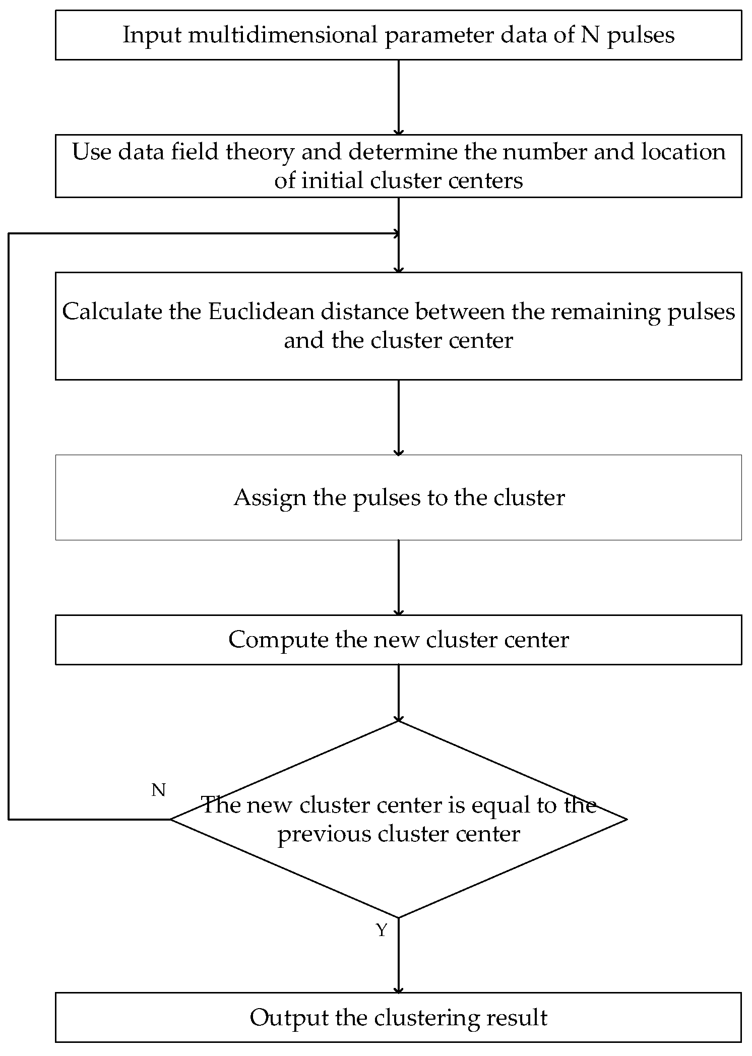
2.1. K-Means Clustering Algorithm Based on Data Fields

K-means clustering is a typical clustering algorithm with wide applications [20,21,22]. The basic principle of a signal sorting clustering algorithm based on data fields is as follows:

Suppose $D=\{D_1,D_2,D_3,\cdots ,D_m\}$ sets of m data are the data to be clustered. K-means clustering finds a partition interval $P_k=\{C_1,C_2,C_3,\cdots ,C_k\}$ that minimizes the objective function $f\left(P_k\right)={\displaystyle \sum _{i=1}^k{\displaystyle {\sum }_{D_{il}\in C_i}d\left(D_{il},M_i\right)}}$. The precise expression is:

$$\exists P_k=\left\{C_1,C_2,C_3,\cdots ,C_k\right\},\mathrm{s}.\mathrm{t}.\min f\left(P_k\right)={\displaystyle \sum _{i=1}^k{\displaystyle {\sum }_{D_{il}\in C_i}d\left(D_{il},M_i\right)}}$$

(1)

In Equation (1), $P_k$ represents the total classification space of data, and $C_1,C_2,C_3,\cdots ,C_k$ is each cluster center in the data space. $D_{il}$ refers to the data points belonging to class $C_i$, and $M_i$ is the cluster center of class $C_i$. With $d\left(D_{il},M_i\right)$, calculate the distance between the data point and the cluster center. The objective function represents the similarity between data, which is usually based on the Euclidean distance. The Euclidean distance formula between $A\left(x_{i1},x_{i2},\cdots ,x_{ik}\right)$ and $B\left(x_{j1},x_{j2},\cdots ,x_{jk}\right)$ is as follows:

$$d\left(i,j\right)={\left({\displaystyle \sum _{k=1}^n{\left|x_{ik}-x_{jk}\right|}^2}\right)}^{\frac{1}{2}}$$

(2)

After data clustering, the center position of class i is obtained as:

$$M_i=\frac{1}{g}{\displaystyle \sum _{i=1}^g{D}_{il}} \left(D_{il}\in C_i\right)$$

(3)

where g represents the number of data in class $C_i$. $M_i$ is the cluster center of class $C_i$, and $D_{il}$ is the data point belonging to class $C_i$. The above is a process of clustering. Then, a new cluster center is calculated, the class is adjusted, and the process is repeated. The classification ends when the sum of squared distances between each data point and each center is the smallest.

The classical K-means algorithm requires selecting the number of clusters and the class central value in advance, which is impossible for unknown radar signal sorting. Secondly, there are often abnormal or wrong data in radar signal sorting, and the K-means algorithm is sensitive to abnormal data, rendering it not directly applicable for radar signal sorting. The data field clustering algorithm can complete the initial clustering without prior knowledge of the data, which provides the prior knowledge required by the K-means clustering algorithm.

Therefore, the data field theory and clustering theory are usually combined in the practical application of clustering algorithms. First, the number of data field clusters is used as the initial number of K-means clusters, and the potential center obtained by data field clustering is used as the initial cluster center of the K-means clustering algorithm. Finally, the K-means clustering algorithm is used to complete the final clustering. The workflow of the algorithm is shown as Figure 1.

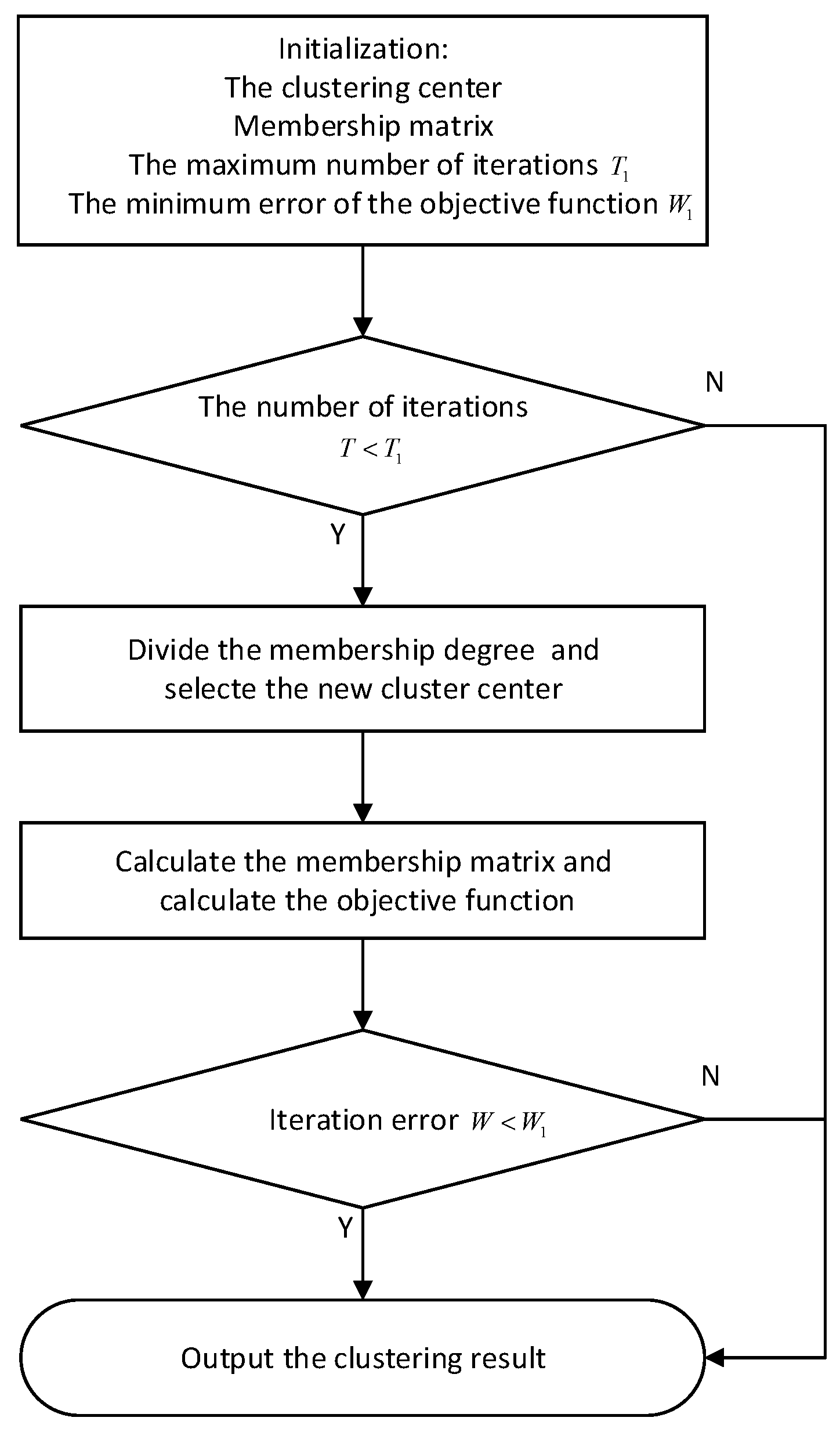
2.2. Fuzzy Clustering Algorithms

The most widely used fuzzy clustering algorithm is FCM clustering, a fuzzy clustering method based on an objective function [23]. Suppose that pulse flow X is divided into C radiation sources, and each radiation source is a class in the clustering algorithm. Each class has a class center $C_i$, and the membership degree of any pulse $x_j$ ($x_j\in X$) belonging to class i is $u_{ij}$. Then, the objective function of the FCM algorithm is as follows:

$$J={\displaystyle \sum _{i=1}^C{\displaystyle \sum _{j=1}^n{u}_{ij}^m}}{\Vert x_j-C_i\Vert }^2$$

(4)

where $\Vert x_j-C_i\Vert$ is the Euclidean distance between pulse $x_j$ and class center $C_i$. $u_{ij}$ is the membership degree, and m is the membership factor. The smaller the objective function J, the better the classification effect of the whole pulse flow.

The constraint function is as follows:

$${\displaystyle \sum _{i=1}^C{u}_{ij}=1,j=1,2,\cdots ,3}$$

(5)

The constraint function of Equation (5) is that the sum of the membership degree of any pulse in the pulse flow to all radiation sources is 1. According to the above analysis, the smaller the objective function J, the better the classification effect of the whole pulse flow. Therefore, the optimization objective of the FCM clustering algorithm is to find the membership matrix $u_{ij}$ and class center $C_i$ through several iterations that minimize the objective function. The iteration formulas of membership matrix $u_{ij}$ and class center $C_i$ are expressed as follows.

$$u_{ij}={\left(\frac{1}{{\displaystyle \sum _{k=1}^C{\left(\frac{\Vert x_j-C_i\Vert }{\Vert x_j-C_k\Vert }\right)}^{\frac{2}{m-1}}}}\right)}^{\frac{1}{m-1}}$$

(6)

$$C_i=\frac{{\displaystyle \sum _{j=1}^n\left(x_j{u}_{ij}^m\right)}}{{\displaystyle \sum _{j=1}^n{u}_{ij}^m}}={\displaystyle \sum _{j=1}^n\frac{u_{ij}^m}{{\displaystyle \sum _{j=1}^n{u}_{ij}^m}}{x}_j}$$

(7)

The steps of the algorithm are shown as Figure 2.

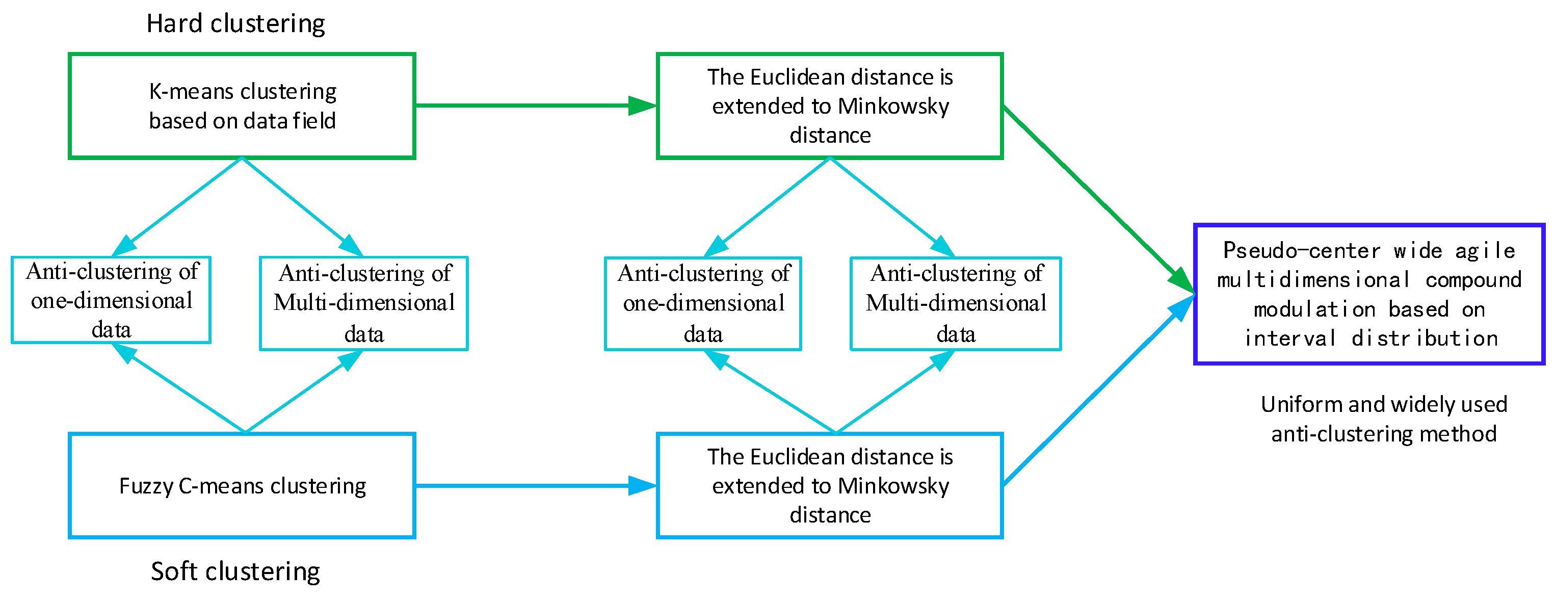
3. Design Principle of Anti-Cluster-Sorting Signal Based on Multi-Dimensional Pseudo-Center Width Agility

The design principle of the anti-cluster-sorting signal is mainly based on the research on signal sorting algorithms. Then, the sorting failure principle is obtained. The failure principle of the sorting algorithm provides theoretical support for the design of the anti-sorting signal and improves the efficiency and success rate of anti-sorting design.

According to the introduction of the clustering algorithm in Section 2, the core step of the clustering algorithm based on the data field theory and the fuzzy clustering algorithm is to judge the similarity of pulses. Euclidean distance is commonly used in clustering algorithms. In this section, the similarity judgment is extended from the Euclidean distance to the Minkowsky distance [24,25,26], which is a more extensive distance calculation method, and its calculation formula is as follows:

$$d_{ij}={\left({\left(x_{i1}-x_{j1}\right)}^q+{\left(x_{i1}-x_{j1}\right)}^q+\cdots +{\left(x_{in}-x_{jn}\right)}^q\right)}^{\frac{1}{q}} \left(q>0\right)$$

(8)

where the Minkowsky distance is the Manhattan distance when q = 1 and the Euclidean distance when q = 2.

Therefore, an anti-clustering method of pseudo-center wide-agile multi-dimensional compound modulation based on interval distribution is proposed in this section for the hard clustering and fuzzy soft clustering methods. A schematic diagram of the analysis and derivation logic is shown in Figure 3.

The core step of the clustering algorithm is to judge the similarity of data points using Euclidean distance and other distance calculation formulas. Therefore, we propose a pseudo-center wide-agile compound modulation method based on interval distribution for the similarity judgment of the clustering algorithm, which is detailed as follows:

① Multi-dimensional indicates the dimension data of PW, RF, and DOA in the pulse descriptor to be clustered and sorted.

② Interval distribution means that the parameters of PW, RF, and DOA obey interval distribution and are no longer fixed values or finite fixed values.

③ Wide agility refers to the jump in the data central values of the same dimension of two adjacent intervals to achieve a large jump in the interval values.

④ Pseudo-center refers to the fact that PW, RF, and DOA from the same radiation source can obviously sort out multiple pseudo-cluster centers in the clustering by the induction sorting algorithm after the interval distribution and wide-agile design. The clustering algorithm will misclassify the signal from the same emitter into multiple emitter signals.

⑤ Compound modulation is designed by combining PW, RF, and DOA with interval distribution and wide-agile design. In this way, the pseudo-cluster centers in the clustering are distinguished more clearly, and the pseudo-cluster centers are prevented from overlapping with each other, which affects the anti-sorting performance of the signal.

According to the above analysis, the wide agility of multi-dimensional parameters is the key step in forming the pseudo-cluster center. Therefore, it is necessary to study the agility of parameters in different clustering algorithms and to use different similarity measurement methods for clustering.

3.1. Failure Principle of K-Means Clustering Based on Data Fields

3.1.1. Euclidean Distance Measures Pulse Similarity

First, the theoretical derivation starts with the analysis of one-dimensional parameters. The central value of the signal PW interval 1 is $x_{10}$, with any value $x\in \left(x_{11},x_{12}\right)$, and the interval is ${\Delta }_1$. The central value of the signal PW interval 2 is $x_{20}$, with any value $x\in \left(x_{21},x_{22}\right)$, and the interval is ${\Delta }_2$. To study the relationship between the agility of parameters and intervals, the PW value is assumed to be $x_A\in \left(x_{11},x_{12}\right)$, and $x_A\to x_{12}$ exists in the signal PW set.

The Euclidean distance between $x_A$ and the central value of interval 1 is:

$$d_{x_A{x}_{10}}=\left|x_A-x_{10}\right|$$

(9)

The Euclidean distance between $x_A$ and the central value of interval 2 is:

$$d_{x_A{x}_{20}}=\left|x_A-x_{20}\right|$$

(10)

Since $x_A\in \left[x_{11},x_{12}\right]$, $d_{x_A{x}_{10}}<d_{x_A{x}_{20}}$.

$$\left|x_A-x_{10}\right|<\left|x_A-x_{20}\right|$$

(11)

Since $x_A\to x_{12}$, Equation (11) can be transformed into:

$$\left|\frac{{\Delta }_1}{2}+x_{10}\right|<\left|\frac{{\Delta }_2}{2}-x_{20}\right|$$

(12)

Therefore,

$$x_{20}-x_{10}>\frac{{\Delta }_1}{2}+\frac{{\Delta }_2}{2}$$

(13)

According to Equation (13), in the case of one-dimensional parameters, multiple pseudo-cluster centers with relative independence and no overlap can be formed when the agility of the central values of two adjacent intervals is at least half the sum of their interval value.

More specifically, if the interval values of two adjacent intervals are equal, i.e., ${\Delta }_1={\Delta }_2=\Delta$,

$$x_{20}-x_{10}>\Delta$$

(14)

Equation (14) shows that with one-dimensional parameters, if the interval values of two adjacent intervals are equal, the agility of the central values of the adjacent intervals is at least one interval, and multiple pseudo-cluster centers with relative independence and no overlap can be formed. The above analysis is performed from one-dimensional parameters to study the relationship between the agility of the interval central value of n-dimensional parameters and the interval.

The central value of the n-dimensional parameter of the signal in interval i is $\text{{}{x}_{i_{j}0}|j\in \left[1,n\right]\text{}}$, and j is any dimension of the n-dimensional parameter in the interval. Any value in interval i is $\text{{}{x}_{i_j}\in \left(x_{i_{j}1},x_{i_{j}2}\right)|j\in \left[1,n\right]\}$, and the interval is $\text{{}{\Delta }_{i_j}|j\in [1,n]\}$. To study the relationship between the agility of parameters and the interval value, it is assumed that there are pulse parameters $\{x_{1_j}\in \left(x_{1_{j}1},x_{1_{j}2}\right)|j\in \left[1,n\right]\}$ and $\{x_{1_j}\to x_{1_{j}2}|j\in \left[1,n\right]\}$ in interval 1.

The Euclidean distance between $x_{1_j}$ and the central value of interval 1 is:

$$d_{x_{1_j}{x}_{1_{j}0}}={\left({\displaystyle \sum _{j=1}^n{\left(x_{1_j}-x_{1_{j}0}\right)}^2}\right)}^{\frac{1}{2}}(j\in \left[1,n\right])$$

(15)

The Euclidean distance between $x_{1_j}$ and the central value of interval 2 is:

$$d_{x_{1_j}{x}_{2_{j}0}}={\left({\displaystyle \sum _{j=1}^n{\left(x_{1_j}-x_{2_{j}0}\right)}^2}\right)}^{\frac{1}{2}}(j\in \left[1,n\right])$$

(16)

Since $\{x_{1_j}\in \left(x_{1_{j}1},x_{1_{j}2}\right)|j\in \left[1,n\right]\}$, $d_{x_{1_j}{x}_{1_{j}0}}<d_{x_{1_j}{x}_{2_{j}0}}$.

$${\left({\displaystyle \sum _{j=1}^n{\left(x_{1_j}-x_{1_{j}0}\right)}^2}\right)}^{\frac{1}{2}}<{\left({\displaystyle \sum _{j=1}^n{\left(x_{1_j}-x_{2_{j}0}\right)}^2}\right)}^{\frac{1}{2}}(j\in \left[1,n\right])$$

(17)

To ensure that $d_{x_{1_j}{x}_{1_{j}0}}<d_{x_{1_j}{x}_{2_{j}0}}$ is always true,

$${\left(x_{1_j}-x_{1_{j}0}\right)}^2<{\left(x_{1_j}-x_{2_{j}0}\right)}^2(j\in \left[1,n\right])$$

(18)

According to the geometric meaning of Equation (18), it can be simplified as:

$$\left|x_{1_j}-x_{1_{j}0}\right|<\left|x_{1_j}-x_{2_{j}0}\right|(j\in \left[1,n\right])$$

(19)

Since $\{x_{1_j}\to x_{1_{j}2}|j\in \left[1,n\right]\}$, Equation (19) can be transformed into:

$$\left|\frac{{\Delta }_{1_j}}{2}+x_{1_{j}0}\right|<\left|\frac{{\Delta }_{2_j}}{2}-x_{2_{j}0}\right|(j\in \left[1,n\right])$$

(20)

Therefore,

$$x_{2_{j}0}-x_{1_{j}0}>\frac{{\Delta }_{1_j}}{2}+\frac{{\Delta }_{2_j}}{2}(j\in \left[1,n\right])$$

(21)

According to Equation (21), in the case of n-dimensional parameters, multiple pseudo-cluster centers with relative independence and no overlap can be formed when the agility of the central values of parameters in any dimension of two adjacent intervals is at least half the sum of the interval value in the respective dimensions.

If the interval values of two adjacent intervals are equal, i.e.,

$${\Delta }_{1_j}={\Delta }_{2_j}=\Delta$$

(22)

Then,

$$x_{2_{j}0}-x_{1_{j}0}>\Delta$$

(23)

Equation (23) shows that for n-dimensional parameters, multiple pseudo-cluster centers with relative independence and no overlap can be formed if the interval values of parameter distribution intervals of any dimension in adjacent intervals are equal, and the agility of parameter central values of any defined dimension in adjacent intervals is at least one interval.

3.1.2. Minkowsky Distance Measures Pulse Similarity

For one-dimensional parameters, the Minkowsky distance is:

$$d={\left({\left(x_{i1}-x_{j1}\right)}^q\right)}^{\frac{1}{q}}=\left|x_{i1}-x_{j1}\right|$$

(24)

According to Equations (9) and (24), in the case of one-dimensional parameters, the calculation formulas of the Minkowsky distance and the Euclidean distance are the same. Therefore, the derivation is roughly the same and will not be repeated.

The following discussion focuses on the relationship between the agility of the parameters and the interval in the case of n-dimensional parameters with the Minkowsky distance calculation similarity.

The central value of the n-dimensional parameter of the signal in interval i is $\text{{}{x}_{i_{j}0}|j\in \left[1,n\right]\text{}}$, and j is any dimension of the n-dimensional parameter in the interval. Any value in interval i is $\text{{}{x}_{i_j}\in \left(x_{i_{j}1},x_{i_{j}2}\right)|j\in \left[1,n\right]\}$, and the interval is $\text{{}{\Delta }_{i_j}|j\in [1,n]\}$. Assuming that there are pulses $\{x_{1_j}\in \left(x_{1_{j}1},x_{1_{j}2}\right)|j\in \left[1,n\right]\}$ and $\{x_{1_j}\to x_{1_{j}2}|j\in \left[1,n\right]\}$ in interval 1, then, the Minkowsky distance between $x_{1_j}$ and the central value of interval 1 is:

$$M_{x_{1_j}{x}_{1_{j}0}}={\left({\displaystyle \sum _{j=1}^n{\left(x_{1_j}-x_{1_{j}0}\right)}^q}\right)}^{\frac{1}{q}}(j\in \left[1,n\right])$$

(25)

The Minkowsky distance between $x_{1_j}$ and the central value of interval 2 is:

$$M_{x_{1_j}{x}_{2_{j}0}}={\left({\displaystyle \sum _{j=1}^n{\left(x_{1_j}-x_{2_{j}0}\right)}^q}\right)}^{\frac{1}{q}}(j\in \left[1,n\right])$$

(26)

Since $\{x_{1_j}\in \left(x_{1_{j}1},x_{1_{j}2}\right)|j\in \left[1,n\right]\}$, $M_{x_{1_j}{x}_{1_{j}0}}<M_{x_{1_j}{x}_{2_{j}0}}$.

$${\left({\displaystyle \sum _{j=1}^n{\left(x_{1_j}-x_{1_{j}0}\right)}^q}\right)}^{\frac{1}{q}}<{\left({\displaystyle \sum _{j=1}^n{\left(x_{1_j}-x_{2_{j}0}\right)}^q}\right)}^{\frac{1}{q}}(j\in \left[1,n\right])$$

(27)

To ensure that $M_{x_{1_j}{x}_{1_{j}0}}<M_{x_{1_j}{x}_{2_{j}0}}$ is always true,

$${\left(x_{1_j}-x_{1_{j}0}\right)}^q<{\left(x_{1_j}-x_{2_{j}0}\right)}^q(j\in \left[1,n\right])$$

(28)

Due to $q>0$ in the calculation of the Minkowsky distance, Equation (28) can be simplified as:

$$\left|x_{1_j}-x_{1_{j}0}\right|<\left|x_{1_j}-x_{2_{j}0}\right|(j\in \left[1,n\right])$$

(29)

Since $\{x_{1_j}\to x_{1_{j}2}|j\in \left[1,n\right]\}$, Equation (29) can be transformed into:

$$\left|\frac{{\Delta }_{1_j}}{2}+x_{1_{j}0}\right|<\left|\frac{{\Delta }_{2_j}}{2}-x_{2_{j}0}\right|(j\in \left[1,n\right])$$

(30)

Therefore,

$$x_{2_{j}0}-x_{1_{j}0}>\frac{{\Delta }_{1_j}}{2}+\frac{{\Delta }_{2_j}}{2}(j\in \left[1,n\right])$$

(31)

According to Equation (31), when the similarity measure is extended from Euclidean distance to the Minkowsky distance in the case of n-dimensional parameters, multiple pseudo-cluster centers with relative independence and no overlap can be formed if the agility of the central values of parameters in any dimension of two adjacent intervals is at least half the sum of the interval value in their respective dimensions.

If the intervals of two adjacent intervals are equal,

$${\Delta }_{1_j}={\Delta }_{2_j}=\Delta$$

(32)

Then,

$$x_{2_{j}0}-x_{1_{j}0}>\Delta$$

(33)

Equation (33) shows that with n-dimensional parameters, multiple pseudo-cluster centers with relative independence and no overlap can be formed if the interval values of parameter distribution intervals of any dimension in two adjacent intervals are equal, and the agility of the parameter central values of any defined dimension in adjacent intervals is at least one interval.

3.2. Failure Principle of FCM Clustering and Sorting

3.2.1. Euclidean Distance Measures Pulse Similarity

The theoretical derivation starts with the analysis of one-dimensional parameters. The central value of the signal PW interval 1 is $x_{10}$, with any value $x\in \left(x_{11},x_{12}\right)$, and the interval is ${\Delta }_1$. The central value of the signal PW interval 2 is $x_{20}$, with any value $x\in \left(x_{21},x_{22}\right)$, and the interval is ${\Delta }_2$. The central values of the two intervals are the two class centers of the FCM clustering algorithm, i.e., the class center $C_1$ of the first class is $x_{10}$, and the class center $C_2$ of the second class is $x_{20}$. Assuming that there are PW values $x_A\in \left(x_{11},x_{12}\right)$ and $x_A\to x_{12}$ in the signal PW set, then, the membership degree of $x_A$ belonging to the first class is:

$$u_{1x_A}=\frac{1}{{\left(\frac{\Vert x_A-x_{10}\Vert }{\Vert x_A-x_{10}\Vert }\right)}^2+{\left(\frac{\Vert x_A-x_{10}\Vert }{\Vert x_A-x_{20}\Vert }\right)}^2}$$

(34)

The membership degree of $x_A$ belonging to the second class is:

$$u_{2x_A}=\frac{1}{{\left(\frac{\Vert x_A-x_{20}\Vert }{\Vert x_A-x_{10}\Vert }\right)}^2+{\left(\frac{\Vert x_A-x_{20}\Vert }{\Vert x_A-x_{20}\Vert }\right)}^2}$$

(35)

Since $x_A\in \left(x_{11},x_{12}\right)$, $u_{1x_A}>u_{2x_A}$.

$$\frac{1}{{\left(\frac{\Vert x_A-x_{10}\Vert }{\Vert x_A-x_{10}\Vert }\right)}^2+{\left(\frac{\Vert x_A-x_{10}\Vert }{\Vert x_A-x_{20}\Vert }\right)}^2}>\frac{1}{{\left(\frac{\Vert x_A-x_{20}\Vert }{\Vert x_A-x_{10}\Vert }\right)}^2+{\left(\frac{\Vert x_A-x_{20}\Vert }{\Vert x_A-x_{20}\Vert }\right)}^2}$$

(36)

Equation (36) can be further simplified as:

$${\left(\frac{\Vert x_A-x_{10}\Vert }{\Vert x_A-x_{10}\Vert }\right)}^2+{\left(\frac{\Vert x_A-x_{10}\Vert }{\Vert x_A-x_{20}\Vert }\right)}^2<{\left(\frac{\Vert x_A-x_{20}\Vert }{\Vert x_A-x_{10}\Vert }\right)}^2+{\left(\frac{\Vert x_A-x_{20}\Vert }{\Vert x_A-x_{20}\Vert }\right)}^2$$

(37)

$${\left(\frac{\Vert x_A-x_{10}\Vert }{\Vert x_A-x_{20}\Vert }\right)}^2<{\left(\frac{\Vert x_A-x_{20}\Vert }{\Vert x_A-x_{10}\Vert }\right)}^2$$

(38)

$$\frac{\Vert x_A-x_{10}\Vert }{\Vert x_A-x_{20}\Vert }<\frac{\Vert x_A-x_{20}\Vert }{\Vert x_A-x_{10}\Vert }$$

(39)

Namely,

$$\Vert x_A-x_{20}\Vert >\Vert x_A-x_{10}\Vert$$

(40)

According to the assumption condition $x_A\to x_{12}$, Equation (40) can be transformed into:

$$\left|\frac{{\Delta }_1}{2}+x_{10}\right|<\left|\frac{{\Delta }_2}{2}-x_{20}\right|$$

(41)

Therefore,

$$x_{20}-x_{10}>\frac{{\Delta }_1}{2}+\frac{{\Delta }_2}{2}$$

(42)

According to Equation (42), in the case of one-dimensional parameters, multiple pseudo-cluster centers with relative independence and no overlap can be formed when the agility of the central values of two adjacent intervals is at least half the sum of their interval value.

More specifically, if the interval values of two adjacent intervals are equal, i.e., ${\Delta }_1={\Delta }_2=\Delta$, then

$$x_{20}-x_{10}>\Delta$$

(43)

Equation (43) shows that in the case of one-dimensional parameters, multiple pseudo-cluster centers with relative independence and no overlap can be formed if the interval values of two adjacent intervals are equal and the agility of the central value of adjacent intervals is at least one interval. The above analysis is conducted from one-dimensional parameters to investigate the relationship between the agility of the interval central value of n-dimensional parameters and the interval.

The central value of the signal n-dimensional parameter in interval i is the clustering center $C_i$ = $\text{{}{x}_{i_{j}0}|j\in \left[1,n\right]\text{}}$ of the FCM algorithm, and j is any dimension of the n-dimensional parameters in the interval. Any value in interval i is $\text{{}{x}_{i_j}\in \left(x_{i_{j}1},x_{i_{j}2}\right)|j\in \left[1,n\right]\}$, and the interval is $\text{{}{\Delta }_{i_j}|j\in [1,n]\}$. Assuming that there are impulse parameters $\{x_{1_j}\in \left(x_{1_{j}1},x_{1_{j}2}\right)|j\in \left[1,n\right]\}$ and $\{x_{1_j}\to x_{1_{j}2}|j\in \left[1,n\right]\}$ in interval 1, the membership degree of $x_{1_j}$ belonging to the first class is:

$$u_{1x_{1_j}}=\frac{1}{{\displaystyle \sum _{k=1}^C{\left(\frac{\Vert x_{1_j}-x_{1_{j}0}\Vert }{\Vert x_{1_j}-C_{k_{j}0}\Vert }\right)}^2}}$$

(44)

The membership degree of $x_{1_j}$ belonging to the second class is:

$$u_{2x_{1_j}}=\frac{1}{{\displaystyle \sum _{k=1}^C{\left(\frac{\Vert x_{1_j}-x_{2_{j}0}\Vert }{\Vert x_{1_j}-x_{k_{j}0}\Vert }\right)}^2}}$$

(45)

Since $\{x_{1_j}\in \left(x_{1_{j}1},x_{1_{j}2}\right)|j\in \left[1,n\right]\}$, $u_{1x_{1_j}}>u_{2x_{1_j}}$, i.e.,

$$\frac{1}{{\displaystyle \sum _{k=1}^C{\left(\frac{\Vert x_{1_j}-x_{1_{j}0}\Vert }{\Vert x_{1_j}-C_{k_{j}0}\Vert }\right)}^2}}>\frac{1}{{\displaystyle \sum _{k=1}^C{\left(\frac{\Vert x_{1_j}-x_{2_{j}0}\Vert }{\Vert x_{1_j}-x_{k_{j}0}\Vert }\right)}^2}}$$

(46)

The final simplification is:

$$\Vert x_{1_j}-x_{1_{j}0}\Vert <\Vert x_{1_j}-x_{2_{j}0}\Vert$$

(47)

According to the assumption condition $\{x_{1_j}\to x_{1_{j}2}|j\in \left[1,n\right]\}$, Equation (47) can be transformed into:

$$\left|\frac{{\Delta }_{1_j}}{2}+x_{1_{j}0}\right|<\left|\frac{{\Delta }_{2_j}}{2}-x_{2_{j}0}\right|(j\in \left[1,n\right])$$

(48)

Therefore,

$$x_{2_{j}0}-x_{1_{j}0}>\frac{{\Delta }_{1_j}}{2}+\frac{{\Delta }_{2_j}}{2}(j\in \left[1,n\right])$$

(49)

According to the derivation of Equation (49), for n-dimensional parameters, multiple pseudo-cluster centers with relative independence and no overlap can be formed when the agility of the central values of parameters in any dimension of two adjacent intervals is at least half the sum of interval value in their respective dimensions. Similarly, if the interval values of parameter distribution intervals of any dimension in two adjacent intervals are equal, multiple pseudo-cluster centers with relative independence and no overlap can be formed when the agility of parameter central values of any defined dimension in adjacent intervals is at least one interval.

3.2.2. Minkowsky Distance Measures Pulse Similarity

Similar to Section 3.1.2, in the case of one-dimensional parameters, the calculation formulas of the Minkowsky distance and the Euclidean distance are the same. Thus, the following derivation is roughly the same and is not repeated here.

The central value of the n-dimensional parameter of the signal in interval i is $\text{{}{x}_{i_{j}0}|j\in \left[1,n\right]\text{}}$, and j is any dimension of the n-dimensional parameter in the interval. Any value in interval i is $\text{{}{x}_{i_j}\in \left(x_{i_{j}1},x_{i_{j}2}\right)|j\in \left[1,n\right]\}$, and the interval is $\text{{}{\Delta }_{i_j}|j\in [1,n]\}$. Assuming that pulses $\{x_{1_j}\in \left(x_{1_{j}1},x_{1_{j}2}\right)|j\in \left[1,n\right]\}$ and $\{x_{1_j}\to x_{1_{j}2}|j\in \left[1,n\right]\}$ exist in interval 1, the membership degree of $x_{1_j}$ belonging to the first class is:

$$u_{1x_{1_j}}=\frac{1}{{\displaystyle \sum _{k=1}^C{\left(\frac{{\left({\displaystyle \sum _{j=1}^n{\left(x_{1_j}-x_{1_{j}0}\right)}^q}\right)}^{\frac{1}{q}}}{{\left({\displaystyle \sum _{j=1}^n{\left(x_{1_j}-x_{k_{j}0}\right)}^q}\right)}^{\frac{1}{q}}}\right)}^2}}$$

(50)

The membership degree of $x_{1_j}$ belonging to the second class is:

$$u_{2x_{1_j}}=\frac{1}{{\displaystyle \sum _{k=1}^C{\left(\frac{{\left({\displaystyle \sum _{j=1}^n{\left(x_{1_j}-x_{2_{j}0}\right)}^q}\right)}^{\frac{1}{q}}}{{\left({\displaystyle \sum _{j=1}^n{\left(x_{1_j}-x_{k_{j}0}\right)}^q}\right)}^{\frac{1}{q}}}\right)}^2}}$$

(51)

Since $\{x_{1_j}\in \left(x_{1_{j}1},x_{1_{j}2}\right)|j\in \left[1,n\right]\}$, $u_{1x_{1_j}}>u_{2x_{1_j}}$, i.e.,

$$\frac{1}{{\displaystyle \sum _{k=1}^C{\left(\frac{{\left({\displaystyle \sum _{j=1}^n{\left(x_{1_j}-x_{1_{j}0}\right)}^q}\right)}^{\frac{1}{q}}}{{\left({\displaystyle \sum _{j=1}^n{\left(x_{1_j}-x_{k_{j}0}\right)}^q}\right)}^{\frac{1}{q}}}\right)}^2}}>\frac{1}{{\displaystyle \sum _{k=1}^C{\left(\frac{{\left({\displaystyle \sum _{j=1}^n{\left(x_{1_j}-x_{2_{j}0}\right)}^q}\right)}^{\frac{1}{q}}}{{\left({\displaystyle \sum _{j=1}^n{\left(x_{1_j}-x_{k_{j}0}\right)}^q}\right)}^{\frac{1}{q}}}\right)}^2}}$$

(52)

Equation (52) can be finally simplified as:

$$\left|x_{1_j}-x_{1_{j}0}\right|<\left|x_{1_j}-x_{2_{j}0}\right|$$

(53)

According to the assumption condition $\{x_{1_j}\in \left(x_{1_{j}1},x_{1_{j}2}\right)|j\in \left[1,n\right]\}$, Equation (53) can be transformed into:

$$\left|\frac{{\Delta }_{1_j}}{2}+x_{1_{j}0}\right|<\left|\frac{{\Delta }_{2_j}}{2}-x_{2_{j}0}\right|(j\in \left[1,n\right])$$

(54)

Therefore,

$$x_{2_{j}0}-x_{1_{j}0}>\frac{{\Delta }_{1_j}}{2}+\frac{{\Delta }_{2_j}}{2}(j\in \left[1,n\right])$$

(55)

According to the derivation of Equation (55), for high-dimensional parameters, multiple pseudo-cluster centers with relative independence and no overlap can be formed when the agility of the central values of parameters in any dimension of two adjacent intervals is at least half the sum of the interval in their respective dimensions. Similarly, if the interval values of parameter distribution intervals of any dimension in two adjacent intervals are equal, then multiple pseudo-cluster centers with relative independence and no overlap can be formed when the agility of parameter central values of any defined dimension in adjacent intervals is at least one interval.

3.3. Signal Design Principles

The sorting failure principle of the K-means clustering algorithm and the fuzzy c-means algorithm based on the data field are analyzed respectively in Section 3.1 and Section 3.2. A kind of sorting algorithm failure principle that can be widely used is obtained. The sorting failure principle points out that when the agile amplitude of the center values of parameters in any dimension of two adjacent intervals is at least half of the sum of the interval intervals in each dimension, multiple pseudo-cluster centers with relative independence and no overlap can be formed. The essence of the failure principle of cluster sorting is to “fake” the correlation of errors between signal pulses through wide interval swiftness and “cheat” the clustering sorting algorithm. The failure principle of cluster sorting provides theoretical guidance and support for the design of an anti-cluster-sorting signal and improves the efficiency and success rate of anti-sorting signal design.

Therefore, in the design of the cluster signal, the signal of the pulse width, the carrier frequency, the pulse repetition interval width of multidimensional parameters such as agility, any dimension parameters, and the adjacent two interval values’ agility amplitude for each dimension under an interval length at least half of the sum can form a relatively independent multiple pseudo-clustering center with no overlap. The signal originally emitted by one radiation source is forged into multiple radiation sources, and then the target of RF stealth and anti-clustering is realized.

4. Signal Simulation Verification and Experiment

In the existing literature, the measurement of signal anti-sorting ability mainly relies on the sorting algorithm to carry out qualitative analysis of a signal sorting simulation. This method cannot accurately describe the anti-sorting ability of the designed signal to the sorting algorithm. In order to quantify the anti-sorting performance of the designed RF stealth signal, the concept of a margin is proposed in this section. After the clustering algorithm, first calculate the sum of the distance between the real central value of each category and the data points contained in each category after clustering. The sum of the distances is then averaged to obtain the average distance between the real cluster center and each data point in the category. We take the average distance of each data point as the margin value of the signal. The calculation formula of the margin is shown in Equation (56):

$$\mathrm{Y}=\frac{1}{z}{{\displaystyle \sum _{i=1}^n{\displaystyle \sum _{j=1}^m\left({\displaystyle \sum _{a=1}^w\left(x_{i{j}_a}-{x^{\prime }}_{i_a}\right)}\right)}}}^{\frac{1}{2}}$$

(56)

where z is the total number of all data points in the clustering simulation, n is the total number of categories after clustering, m is the total number of data points contained in each category, and w is the dimension of each data point. $x_{i{j}_a}$ is the ath-dimension value of the j-th data point in class i. ${x^{\prime }}_{i_a}$ is the ath-dimension value of the center value of class i in the real category.

It can be seen from the calculation process that the larger the margin value is, the farther the difference between the data points in the cluster and the real cluster center and the better the anti-sorting performance of the signal are. The smaller the margin value of the signal is, the closer the difference between the data points in the cluster and the real cluster center and the worse the anti-sorting performance of the signal are. The simulation experiment environment was a Windows10 64-bit operating system. The simulated computer parameters were as follows: the processor was a Core i7-9750H, the main frequency was 2.60 GHz, and the memory was 8 GB.

4.1. Simulation Verification of Signal Design Principle

The principle of anti-clustering signal design points out that in the case of N-dimensional parameters, multiple pseudo-clustering centers with relative independence and no overlap can be formed when the agile amplitude of the center values of parameters in any dimension of two adjacent intervals is at least half of the sum of the interval intervals in the respective dimensions. In particular, if the interval values of the parameter distribution intervals of any dimension in two adjacent intervals are equal, then multiple pseudo-cluster centers with relative independence and no overlap can be formed when the agile amplitude of the parameter center values of any definite dimension in the adjacent interval is at least one interval. In order to verify the correctness of the signal design principle, a comparative simulation is carried out in this section. The specific principles of the simulation are as follows:

① The simulation mainly simulates two kinds of signals with a wide interval agility and a non-wide interval agility of the parameter center value.

② The central value’s wide interval agility of the multi-dimensional signal parameters can be divided into two aspects: parameter multi-dimensionalization and parameter wide interval agility. The multi-dimensionalization of parameters mainly refers to the modulation of the three dimensions of the signal PW, the carrier frequency, and the DOA. Parameter wide-interval agility means that the agility of the central values of the signal parameters of any dimension in two adjacent intervals is greater than the sum of half of the respective intervals.

③ The central value of signal parameters with a non-wide interval agility means that the central value agility of the signal parameters in any dimension in two adjacent intervals is less than half the sum of their respective intervals.

Through the above three simulation setting principles, the simulation is more intuitive in showing that the anti-clustering signal designed by the pseudo-center wide-agile multi-dimensional composite modulation signal design method proposed in this paper can make the clustering sorting algorithm invalid. They provide theoretical support for the design of the anti-clustering signal and effectively guides the design of the anti-clustering signal.

The simulation parameters are set in

Table 1. Parameter setting of signal simulation.

Serial Number	Parameter Type	Center Value with Wide-Interval Agility			Center Value without Wide-Interval Agility
		Center Value	Parameter Variation Interval	Interval Length	Center Value	Parameter Variation Interval	Interval Length
1	PW	$15 \mathsf{\mu }\mathrm{s}$	$\left[13 \mathsf{\mu }\mathrm{s},17 \mathsf{\mu }\mathrm{s}\right]$	$4 \mathsf{\mu }\mathrm{s}$	$15 \mathsf{\mu }\mathrm{s}$	$\left[13 \mathsf{\mu }\mathrm{s},17 \mathsf{\mu }\mathrm{s}\right]$	$4 \mathsf{\mu }\mathrm{s}$
2		$20 \mathsf{\mu }\mathrm{s}$	$\left[18 \mathsf{\mu }\mathrm{s},22 \mathsf{\mu }\mathrm{s}\right]$	$4 \mathsf{\mu }\mathrm{s}$	$18 \mathsf{\mu }\mathrm{s}$	$\left[16 \mathsf{\mu }\mathrm{s},20 \mathsf{\mu }\mathrm{s}\right]$	$4 \mathsf{\mu }\mathrm{s}$
3		$25 \mathsf{\mu }\mathrm{s}$	$\left[23 \mathsf{\mu }\mathrm{s},27 \mathsf{\mu }\mathrm{s}\right]$	$4 \mathsf{\mu }\mathrm{s}$	$20 \mathsf{\mu }\mathrm{s}$	$\left[18 \mathsf{\mu }\mathrm{s},22 \mathsf{\mu }\mathrm{s}\right]$	$4 \mathsf{\mu }\mathrm{s}$
4	DOA	${40}^{\circ }$	$\left[{39.5}^{\circ },{40.5}^{\circ }\right]$	$1^{\circ }$	${40}^{\circ }$	$\left[{39.5}^{\circ },{40.5}^{\circ }\right]$	$1^{\circ }$
5		${42}^{\circ }$	$\left[{41.5}^{\circ },{42.5}^{\circ }\right]$	$1^{\circ }$	${41}^{\circ }$	$\left[{40.5}^{\circ },{41.5}^{\circ }\right]$	$1^{\circ }$
6		${44}^{\circ }$	$\left[{43.5}^{\circ },{44.5}^{\circ }\right]$	$1^{\circ }$	${41.5}^{\circ }$	$\left[{41}^{\circ },{42}^{\circ }\right]$	$1^{\circ }$
7	RF	3.5 GHz	$\left[3.25 \mathrm{GHz},3.75 \mathrm{GHz}\right]$	0.5 GHz	3.5 GHz	$\left[3.25 \mathrm{GHz},3.75 \mathrm{GHz}\right]$	0.5 GHz
8		4.1 GHz	$\left[3.85 \mathrm{GHz},4.35 \mathrm{GHz}\right]$	0.5 GHz	3.9 GHz	$\left[3.65 \mathrm{GHz},4.15 \mathrm{GHz}\right]$	0.5 GHz
9		4.7 GHz	$\left[4.45 \mathrm{GHz},4.95 \mathrm{GHz}\right]$	0.5 GHz	4.3 GHz	$\left[4.05 \mathrm{GHz},4.55 \mathrm{GHz}\right]$	0.5 GHz

.

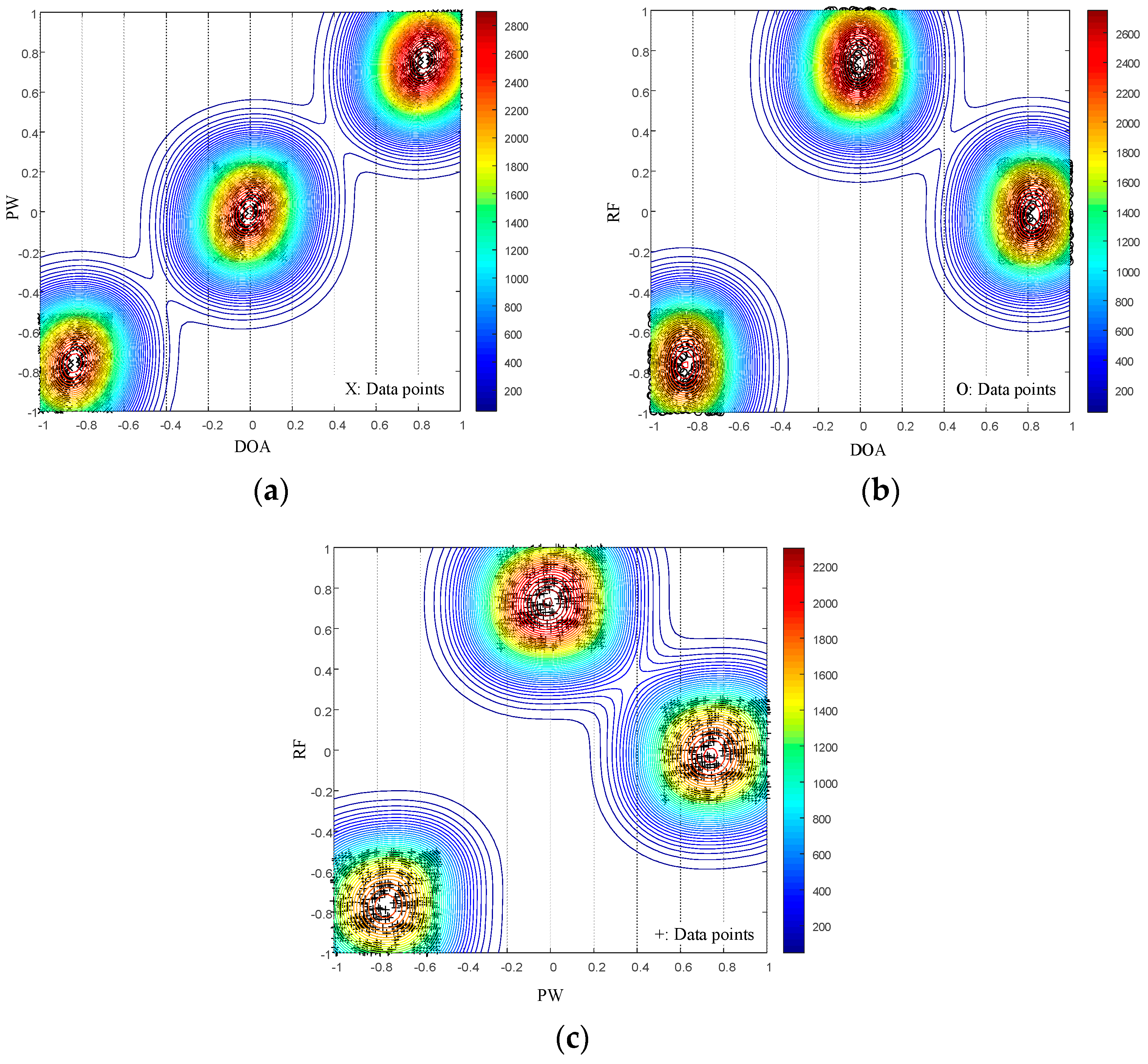
4.1.1. Simulation Verification of K-Means Clustering Based on the Data Field

The K-means clustering diagram based on the data field is shown in Figure 4 and Figure 5.

As shown in Figure 4, with the parameter design method of the three-dimensional pseudo-center wide-agile composite modulation proposed in this paper, the data field clustering algorithm divides the signals sent by radar into three cluster centers in the PW-DOA, RF-DOA, and RF-PW dimensions. In the clustering algorithm, the signal originally sent by one radar is sorted into the signal sent by three radiation sources, and one radiation source is incorrectly sorted into three radiation sources. The clustering algorithm was successfully “tricked”, and the algorithm sorting failed. The radar signal achieves the target of radio frequency stealth. The signal design principle of pseudo-center wide-agile multi-dimensional compound modulation correctly guides the design of the anti-cluster-sorting signal. As shown in Figure 5, if the anti-clustering algorithm proposed in this paper is not used when designing the signal parameters, the signal is sorted into two cluster centers in the RF-DOA and RF-PW dimensions and a cluster center in the PW-DOA dimension. The clustering algorithm can perform proper sorting in the PW-DOA dimension, and we cannot achieve the anti-clustering sorting. The comparison of Figure 4 and Figure 5 verifies the correctness of the signal design principle and proves that the design principle can provide strong theoretical support for the anti-sorting signal design.

4.1.2. Simulation Verification of FCM Clustering

The FCM clustering diagrams are shown in Figure 6 and Figure 7.

According to Figure 6, the parameters modulated by the FCM clustering algorithm by the proposed three-dimensional pseudo-center wide-agile joint design method are sorted into three classes in the PW-DOA, RF-DOA and RF-PW dimensions, since one emitter is incorrectly sorted into three sources. The designed signal realizes RF stealth and has strong anti-clustering and sorting ability. According to the FCM clustering sorting diagram in Figure 7, the signal parameters that are not modulated by the method proposed are clustered, and the dimensions of PW-DOA and PW-RF are the two clustering centers. Although the DOA-RF dimension is sorted into two centers, most of the data between the two cluster centers belong to one of the categories, and the parameters of the three regions may be sorted into one category. The clustering diagram of three different dimensions, (a), (b), and (c), in Figure 7 is further analyzed. The data of the three regions in the figure coincide with each other, which has the potential to be sorted into one class and cannot realize the anti-clustering sorting. The comparison of Figure 6 and Figure 7 verifies the correctness of the sorting failure principle.

4.2. Comparison Simulation with Random Interference Pulse Anti-Sorting Signal

In the field of signal anti-sorting, changing the signal composition of the electromagnetic environment by introducing random interference pulses is also considered to be one of the signals with better anti-clustering sorting performance [18,19]. In this section, we take the random interference pulse anti-sorting signal as an example and make a qualitative and quantitative comparison of the signal anti-sorting ability in terms of the K-means clustering algorithm based on the data field and the margin, respectively.

4.2.1. Comparative Simulation of K-Means Clustering Algorithm Based on Data Field for Signal Sorting

The parameter settings of the anti-sorting signal designed in this paper and the random interference pulse are shown in

Table 2. The simulation parameters settings of anti-sorting signal designed in the paper.

Serial Number	Parameter Type	Center Value with Wide-Interval Agility
		Center Value	Parameter Variation Interval	Interval Length
1	PW	$15 \mathsf{\mu }\mathrm{s}$	$\left[13 \mathsf{\mu }\mathrm{s},17 \mathsf{\mu }\mathrm{s}\right]$	$4 \mathsf{\mu }\mathrm{s}$
2		$20 \mathsf{\mu }\mathrm{s}$	$\left[18 \mathsf{\mu }\mathrm{s},22 \mathsf{\mu }\mathrm{s}\right]$	$4 \mathsf{\mu }\mathrm{s}$
3		$25 \mathsf{\mu }\mathrm{s}$	$\left[23 \mathsf{\mu }\mathrm{s},27 \mathsf{\mu }\mathrm{s}\right]$	$4 \mathsf{\mu }\mathrm{s}$
4	DOA	${40}^{\circ }$	$\left[{39.5}^{\circ },{40.5}^{\circ }\right]$	$1^{\circ }$
5		${42}^{\circ }$	$\left[{41.5}^{\circ },{42.5}^{\circ }\right]$	$1^{\circ }$
6		${44}^{\circ }$	$\left[{43.5}^{\circ },{44.5}^{\circ }\right]$	$1^{\circ }$
7	RF	3.5 GHz	$\left[3.25 \mathrm{GHz},3.75 \mathrm{GHz}\right]$	0.5 GHz
8		4.1 GHz	$\left[3.85 \mathrm{GHz},4.35 \mathrm{GHz}\right]$	0.5 GHz
9		4.7 GHz	$\left[4.45 \mathrm{GHz},4.95 \mathrm{GHz}\right]$	0.5 GHz

and

Table 3. Simulation parameter setting of random interference pulse signal.

Serial Number	Parameter Type	Center Value with Wide-Interval Agility
		Center Value	Parameter Variation Interval	Interval Length
1	PW	$20 \mathsf{\mu }\mathrm{s}$	$\left[13 \mathsf{\mu }\mathrm{s},27 \mathsf{\mu }\mathrm{s}\right]$	$14 \mathsf{\mu }\mathrm{s}$
2	DOA	${42}^{\circ }$	$\left[{39.5}^{\circ },{44.5}^{\circ }\right]$	$5^{\circ }$
3	RF	4.1 GHz	$\left[3.25 \mathrm{GHz},4.95 \mathrm{GHz}\right]$	1.7 GHz

.

The simulation results are shown in Figure 4 and Figure 8.

As can be seen from Figure 4, the anti-sorting signal designed in this paper is sorted into three clustering centers in the three dimensions of the clustering algorithm PW-DOA, RF-DOA, and RF-PW, and the clustering center splitting is realized. The signal from one radar is wrongly sorted into multiple radar signals, which deceives the clustering sorting algorithm and realizes the anti-sorting target of radar. As shown in Figure 8, although the random interference pulse anti-sorting signal realizes the jump of signal parameters in a certain area, it will not cause the clustering center to split in the clustering algorithm, and the clustering algorithm cannot be tricked. Therefore, the anti-clustering sorting ability of the random interference pulse signal is weak.

4.2.2. Comparison Simulation of Signal Sorting Based on Margin

The parameter settings of the designed signal and random interference pulse signal are shown in Table 2 and Table 3. Each of these signals contains 10,000 pulses. In order to ensure that the margin value can more accurately reflect the anti-sorting performance of the signal, the Monte Carlo simulation is carried out 1000 times, and 50 of these are randomly selected for drawing, as shown in Figure 9.

As can be seen from Figure 9, the margin value of the anti-sorting signal designed in this section is significantly higher than that of the random interference pulse signal. This shows that the anti-sorting performance of the signal designed according to the anti-sorting signal design principle of the pseudo-center wide-agility multi-dimensional composite modulation proposed in this paper is obviously better than that of the random interference pulse signal.

4.3. Contrast Experiment of Signal Sorting Based on Experimental System

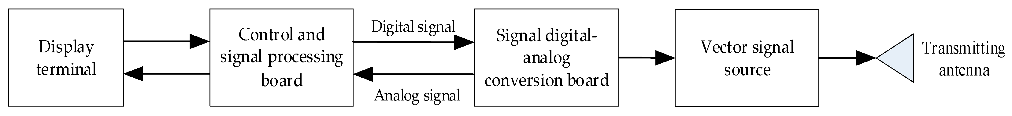
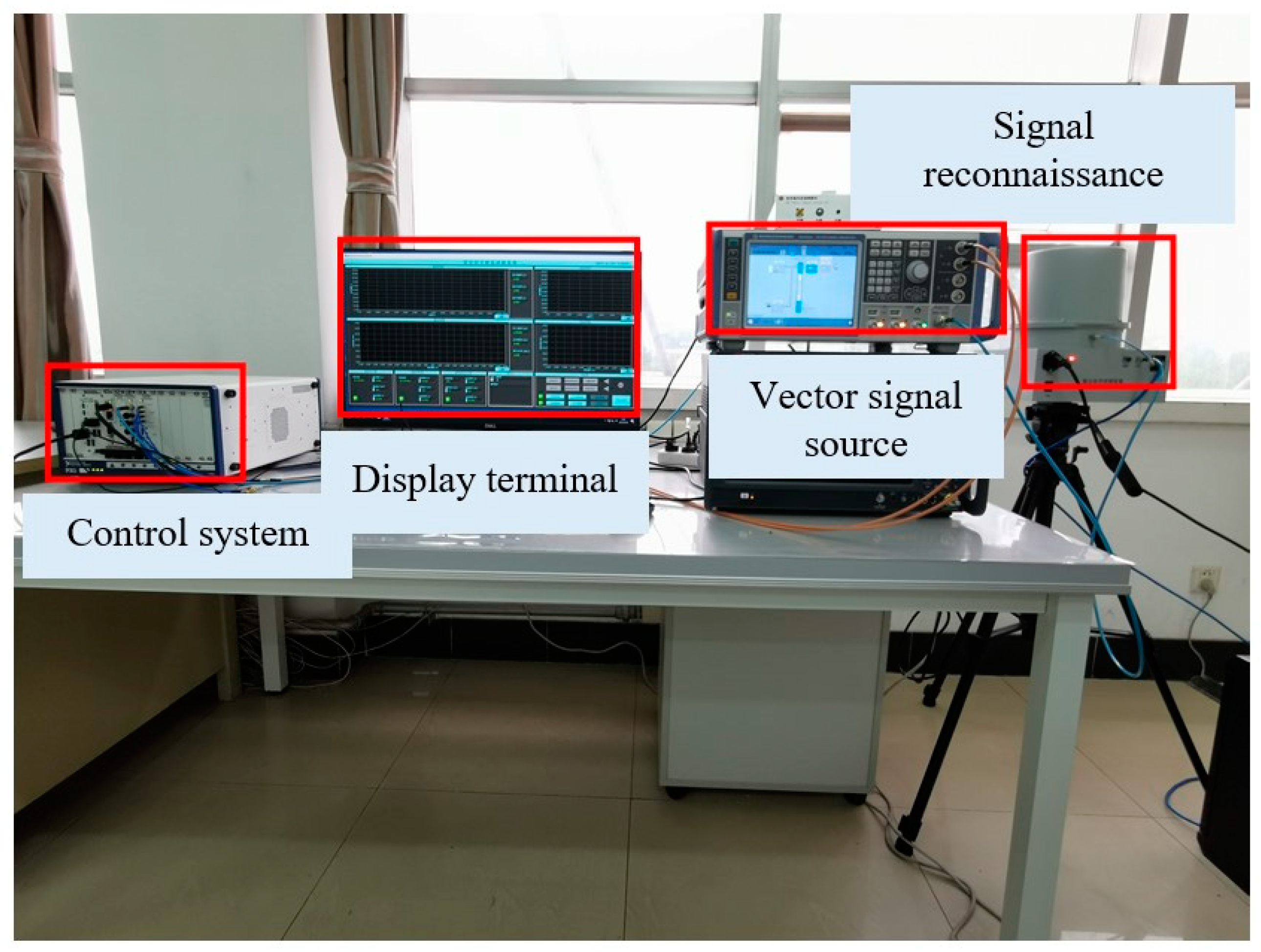
4.3.1. Introduction to Experimental System

The experimental system is composed of two parts: the first part is the signal transmission subsystem, and the second part is the signal reconnaissance subsystem. The signal transmission subsystem is composed of a vector signal source, a signal digital-analog conversion board, a control and signal processing board, and a display terminal. The signal transmitting subsystem uses remote-control technology to integrate the signal digital–analog conversion, signal processing, and signal generation into a system. Then, the vector signal source transmits a waveform file prepared by MATLAB code. The structure and composition of the signal transmission subsystem is shown in Figure 10. The signal reconnaissance subsystem is mainly composed of a receiving antenna, an electronic equipment host, a display control host, a power extension, a triangle bracket, and several cables. It delivers real-time measurement, processing, sorting, and identification of the radio frequency (RF), pulse width (PW), pulse amplitude (PA), and TOA parameters of the radar target radiation source signal. A schematic diagram is shown in Figure 11.

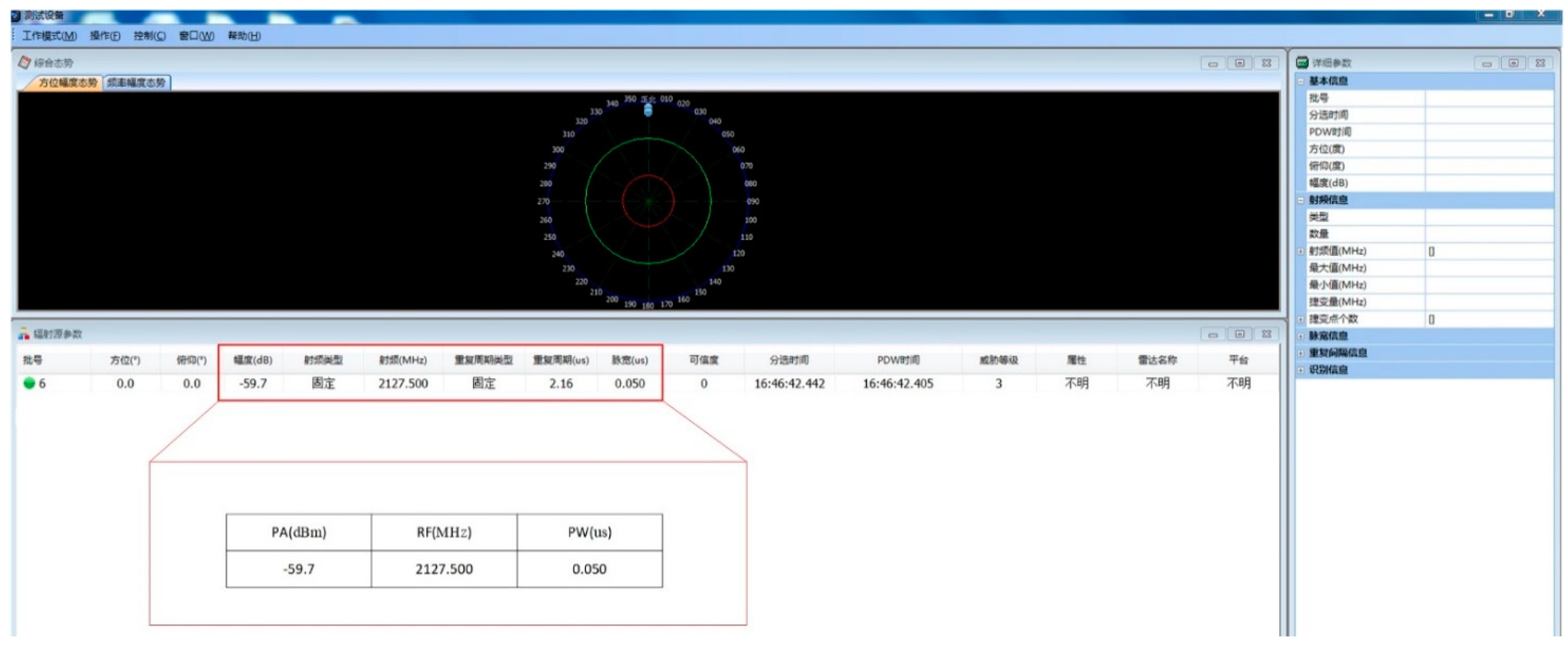
4.3.2. Sorting Contrast Experiment

First, signals are generated by the signal transmitting subsystem in this experiment. Second, in order to avoid the impact of the noise in the natural environment on the experiment, the signal generated by the vector signal source is not transmitted by the horn antenna, received by the antenna, and transmitted to the signal processing engine, but directly transmitted to the signal processing host of the signal sorting subsystem through the cable. The specific connection of the experimental system is shown in Figure 12.

As the photo format is limited, the display terminal interface of the signal sorting system is shown in Figure 13.

In Figure 13, each parameter of the signal in the interface diagram of the signal sorting experimental system is introduced. When the signal is successfully sorted by the sorting experiment system, various parameters such as the carrier frequency and pulse repetition interval will be displayed on the interface of the sorting experiment system. Each line of the interface shows the parameters of a radar signal sorted by the sorting test system. The number of lines in the interface represents the number of radiation source signals that have been sorted out by the sorting experiment system.

Meanwhile, there is a circle on the black plane at the top of the interface of the sorting experiment system. This circle is the signal sorting experiment system showing the direction of the emitter that has been sorted. The circle is divided into 360 degrees into 36 equal parts. It goes clockwise, from 10 degrees to 20 degrees to 30 degrees, all the way to 360 degrees. The sorting system determines the orientation of the source signal, which is shown in a circle on a black plane. It can be seen from Figure 12 that the antenna in the signal sorting test system is a circular omnidirectional antenna. The determination of the signal azimuth in the sorting test system depends on the comparison of amplitude between two antennas. However, in practice, the whole system has only one antenna, and there is no way to determine the azimuth of the radiation source. Therefore, the sorting experiment system does not show the radiation source azimuth in this paper. Considering the actual situation, the pulse width, pulse amplitude, and carrier frequency of the signal are mainly set, and the arrival direction of the signal is not set in the experiment of this paper. Therefore, the failure of the sorting test system to judge the direction of the radiation source will not affect the experimental results of the paper. In this paper, the results of the signal sorting experiment using the sorting experiment system are still true and credible.

Due to hardware limitations of the signal generation subsystem, the simulation parameter settings are slightly different from those in the simulation verification stage in Section 4.1. The specific settings are shown in

Table 4. Parameter setting of sorting contrast experiment.

Serial Number	Parameter Type	Center Value with Wide-Interval Agility			Center Value without Wide-Interval Agility
		Center Value	Parameter Variation Interval	Interval Length	Center Value	Parameter Variation Interval	Interval Length
1	PW	$0.035 \mathsf{\mu }\mathrm{s}$	$\left[0.025 \mathsf{\mu }\mathrm{s},0.045 \mathsf{\mu }\mathrm{s}\right]$	$0.02 \mathsf{\mu }\mathrm{s}$	$0.035 \mathsf{\mu }\mathrm{s}$	$\left[0.025 \mathsf{\mu }\mathrm{s},0.045 \mathsf{\mu }\mathrm{s}\right]$	$0.02 \mathsf{\mu }\mathrm{s}$
2		$0.055 \mathsf{\mu }\mathrm{s}$	$\left[0.045 \mathsf{\mu }\mathrm{s},0.065 \mathsf{\mu }\mathrm{s}\right]$	$0.02 \mathsf{\mu }\mathrm{s}$	$0.050 \mathsf{\mu }\mathrm{s}$	$\left[0.04 \mathsf{\mu }\mathrm{s},0.06 \mathsf{\mu }\mathrm{s}\right]$	$0.02 \mathsf{\mu }\mathrm{s}$
3		$0.075 \mathsf{\mu }\mathrm{s}$	$\left[0.065 \mathsf{\mu }\mathrm{s},0.085 \mathsf{\mu }\mathrm{s}\right]$	$0.02 \mathsf{\mu }\mathrm{s}$	$0.065 \mathsf{\mu }\mathrm{s}$	$\left[0.065 \mathsf{\mu }\mathrm{s},0.085 \mathsf{\mu }\mathrm{s}\right]$	$0.02 \mathsf{\mu }\mathrm{s}$
4	PA	−5 dBm	[−10 dBm,0 dBm]	10 dBm	−5 dBm	[−10 dBm,0 dBm]	10 dBm
5		5 dBm	[0 dBm,10 dBm]	10 dBm	0 dBm	[−5 dBm,5 dBm]	10 dBm
6		15 dBm	[10 dBm,20 dBm]	10 dBm	5 dBm	[0 dBm,10 dBm]	10 dBm
7	RF	2.0 GHz	$\left[1.8\mathrm{GHz},2.2\mathrm{GHz}\right]$	0.4 GHz	2.0 GHz	$\left[1.8\mathrm{GHz},2.2\mathrm{GHz}\right]$	0.4 GHz
8		2.4 GHz	$\left[2.2\mathrm{GHz},2.6\mathrm{GHz}\right]$	0.4 GHz	2.3 GHz	$\left[2.1\mathrm{GHz},2.5\mathrm{GHz}\right]$	0.4 GHz
9		2.8 GHz	$\left[2.6\mathrm{GHz},3.0\mathrm{GHz}\right]$	0.4 GHz	2.6 GHz	$\left[2.4\mathrm{GHz},2.8\mathrm{GHz}\right]$	0.4 GHz

.

In Table 4, PW is the abbreviation for pulse width, PA is the abbreviation for pulse amplitude, and RF is the abbreviation for radio frequency. The sorting results are shown in Figure 14 and Figure 15.

Figure 14 shows the signal sorting results generated by the signal sorting experimental system using the anti-sorting signal design method proposed in this paper. It can be seen from Figure 14 that there are three rows of parameters in the interface of the sorting experimental system, indicating that the sorting experimental system has sorted out three radar signals. The first signal amplitude is −60.3 dBm, the carrier frequency is 2065 MHZ, and the pulse width is 0.05 us. The second signal amplitude is −48.7 dBm, the carrier frequency is 2821.5 MHz, and the pulse width is 0.037 us. The third signal amplitude is −49.0 dBm, the carrier frequency is 2437.5 MHz, and the pulse width is 0.075 us. The sorting test system incorrectly sorts the signals originally sent by one radar into three radar signals. That is, one radar is incorrectly sorted into three radars. The clustering algorithm is working incorrectly. The sorting results in Figure 14 directly illustrate that the anti-clustering signal design method proposed in this paper can be used to design signals with anti-clustering and sorting ability of RF stealth.

Figure 15 shows the sorting results generated by the signal sorting experimental system without applying the anti-sorting signal design method proposed in this paper. As can be seen from Figure 15, there is a row of parameters in the interface of the sorting experimental system, indicating that the sorting experimental system has sorted out a radar signal. The amplitude of the signal is −59.7 dBm, the carrier frequency is 2127.5 MHz, and the pulse width is 0.05 us. The sorting system can correctly sort out the signals that are not designed using the design method proposed in this paper. It can be seen from the comparison of Figure 14 and Figure 15 that the signal design principle proposed in this paper can design signals with anti-cluster-sorting ability. For such signals, even the efficient sorting test system cannot achieve effective sorting identification.

5. Conclusions

Pre-sorting plays a key role in signal sorting. In this study, two clustering algorithms, hard clustering and fuzzy soft clustering, were studied in detail, especially the K-means clustering algorithm and the FCM clustering algorithm based on the data field. A unified and widely used design principle of anti-clustering sorting signal was proposed to guide the design of RF stealth anti-sorting signals. For the data similarity measure step that must be performed in the clustering algorithm, the design method of a multi-dimensional pseudo-center wide-agile composite modulation anti-clustering signal based on interval distribution was proposed. It should be noted that in the case of multi-dimensional parameters, when the agility of the central values of the parameters in any dimension of two adjacent intervals is at least half the sum of the interval lengths in the respective dimensions, multiple pseudo-cluster centers with relative independence and no overlap can be formed, and the anti-cluster classification of radar signals can be realized. Then, the correctness of the design principle of anti-cluster sorting was verified with theory and practice with a formula derivation and signal simulation. Then, by comparing the simulation with the random interference pulse method, which is the main anti-clustering sorting method, the simulation strongly proved that the anti-clustering signal design principle proposed in this paper guides the design of the signal with stronger anti-sorting performance than the random interference pulse signal. The signal design principle can provide theoretical support for the design of anti-sorting signals, which is beneficial to improving the efficiency and success rate of anti-sorting design.

References

1. Jia, J.; Han, Z.; Liang, Y.; Liu, L.; Wang, X. Design of Multi-Parameter Compound Modulated RF Stealth Anti-Sorting Signals Based on Hyperchaotic Interleaving Feedback. Entropy 2022, 24, 1283. [Google Scholar] [CrossRef] [PubMed]
2. Jia, J.W.; Liu, L.M.; Han, Z.Z.; Xie, H. A survey on waveform design technology of RF stealth radar. Electron. Opt. Control 2022, 29, 57–64+78. [Google Scholar]
3. Zhao, X.T.; Zhou, J.J. Improved MUSIC algorithm for MIMO radar with low intercept. Syst. Eng. Electron. 2022, 44, 490–497. [Google Scholar]
4. Sun, Y.B. Low probability of intercept waveform with rejection capability of spread spectrum parameter measurements. Telecommun. Eng. 2021, 61, 821–826. [Google Scholar]
5. Chang, W. Design of synthetic aperture radar low-intercept radio frequency stealth. J. Syst. Eng. Electron. 2020, 31, 64–72. [Google Scholar] [CrossRef]
6. Yang, Y.X.; Wang, D.X.; Huang, Q. Design Method of Radio Frequency Stealth Frequency Hopping Communications Based on Four-Dimensional Hyperchaotic System. J. Astronaut. 2020, 41, 1341–1349. [Google Scholar]
7. Fan, Y.C. Research on RF Stealth Waveform Design of Airborne Battlefield Surveillance Radar; China Academic of Electronics and Information Technology: Beijing, China, 2021. [Google Scholar]
8. Liu, L.T.; Wang, L.L.; Chen, T. Non-parametric radar signal sorting algorithm based on improved DSets. Chin. J. Ship Res. 2021, 16, 232–238. [Google Scholar]
9. Sui, J.P.; Liu, Z.; Liu, L.; Li, X. Progress in radar emitter signal deinterleaving. J. Radars 2022, 11, 418–433. [Google Scholar]
10. Jiang, Z.Y.; Sun, S.Y.; Li, H.W.; Guang, L. A method for deinterleaving based on JANET. J. Univ. Chin. Acad. Sci. 2021, 38, 825–831. [Google Scholar]
11. Jia, J.; Han, Z.; Liu, L.; Xie, H.; Lv, M. Research on the Sequential Difference Histogram Failure Principle Applied to the Signal Design of Radio Frequency Stealth Radar. Electronics 2022, 11, 2192. [Google Scholar] [CrossRef]
12. Jia, J.; Han, Z.; Liu, L.; Xie, H.; Lv, M. Research on the SDIF Failure Principle for RF Stealth Radar Signal Design. Electronics 2022, 11, 1117. [Google Scholar] [CrossRef]
13. Yu, Q.; Bi, D.P.; Chen, L. Jamming Technology of Research Based on PRI Parameter Separation of Signal to ELINT System. Fire Control. Command. Control. 2016, 41, 143–147. [Google Scholar]
14. Dai, S.B.; Lei, W.H.; Cheng, Y.Z. Electronic Anti-Reconnaissance Based on TOA Analysis. Electron. Inf. Warf. Technol. 2014, 29, 4. [Google Scholar]
15. Wang, F.; Liu, J.F. LPS design of pulse repetition interval for formation radars. Inf. Technol. 2019, 3, 14–18+23. [Google Scholar]
16. Nan, H.; Peng, S.; Yu, J.; Wang, X. Pulse interference method against PRI sorting. J. Eng. 2019, 2019, 5732–5735. [Google Scholar] [CrossRef]
17. Sun, Z.Y.; Jiang, Q.X.; Bi, D.P. A technology for anti-reconnaissance based on factional quasi orthogonal waveform. Mod. Radar 2015, 37, 7. [Google Scholar]
18. Zhang, B.Q.; Wang, W.S. Anti-Clustering Analysis of Anti-Reconnaissance Based on Full Pulse Information Extraction. Electron. Inf. Warf. Technol. 2017, 32, 19–25. [Google Scholar]
19. Wang, W.S.; Ban, X.D.; Long, X.B. Research on Count-Reconnaissance of Emitters Based on Ant- ISODATA Clustering Analysis. Electron. Inf. Warf. Technol. 2012, 27, 41–45+68. [Google Scholar]
20. Chen, J.; Wang, Y.; Li, J.; Long, W. Tensor Decomposition and K⁃means Clustering Based Array Diagnosis for MIMO Radar in Impulsive Noise Environment. Acta Electron. Sin. 2021, 49, 2315–2322. [Google Scholar]
21. Hou, F.; Yao, Z.; Yang, J.; Li, Y.; Wang, Z. A fast detection method of frequency hopping signal based on K-means clustering. Telecommun. Eng. 2022, 62, 199–205. [Google Scholar]
22. Yang, L. Radio sorting and recognition technology based on K-means clustering for subtle features. Telecommun. Eng. 2022, 62, 1149–1154. [Google Scholar]
23. Gao, Y.; Yang, C.; Wang, Z.; Luo, S.; Pan, J. Robust Fuzzy C-means Clustering Algorithm Integrating Between-cluster Information. J. Electron. Inf. Technol. 2019, 41, 1114–1121. [Google Scholar]
24. Huang, C. Analysis of Typical Cluster Methods in Radar Signal Sorting. Electron. Inf. Warf. Technol. 2017, 32, 1–4+62. [Google Scholar]
25. Guo, J.; Chen, J. Clustering approach for deinterleaving unknown radar signals. Syst. Eng. Electron. 2006, 28, 853–863. [Google Scholar]
26. Peng, G.; Yuan, X.; Liu, W. A Survey of Clustering and Sorting Algorithms for Radar Source Signals. Radar Sci. Technol. 2019, 17, 485–492. [Google Scholar]
Figure 1. Flow chart of the K-means clustering algorithm based on data fields.
Electronics 11 04027 g001
Figure 2. Flow chart of the FCM clustering algorithm.
Electronics 11 04027 g002
Figure 3. The derivation logic diagram in this paper.
Electronics 11 04027 g003
Figure 4. Two-dimensional distribution of the proposed signal parameter’s equipotential lines with three-dimensional pseudo-center wide-agile composite modulation. (a) Two-dimensional diagram of the PW-DOA equipotential line. (b) Two-dimensional diagram of the RF-DOA equipotential line. (c) Two-dimensional diagram of the RF-PW equipotential line.
Electronics 11 04027 g004
Figure 5. Two-dimensional distribution of signal parameter’s equipotential lines without three-dimensional pseudo-center wide-agile composite modulation. (a) Two-dimensional diagram of the PW-DOA equipotential line. (b) Two-dimensional diagram of the RF-DOA equipotential line. (c) Two-dimensional diagram of the RF-PW equipotential line.
Electronics 11 04027 g005
Figure 6. FCM clustering diagrams of the proposed three-dimensional pseudo-center wide-agile joint design parameters. (a) PW-DOA two-dimensional cluster diagram. (b) PW-RF two-dimensional cluster diagram. (c) DOA-RF two-dimensional cluster diagram. (d) The change of the objective function.
Electronics 11 04027 g006
Figure 7. FCM clustering diagrams of signal parameters designed without three-dimensional pseudo-center wide-agile composite modulation. (a) PW-DOA two-dimensional cluster diagram. (b) PW-RF two-dimensional cluster diagram. (c) DOA-RF two-dimensional cluster diagram. (d) The change of the objective function.
Electronics 11 04027 g007aElectronics 11 04027 g007b
Figure 8. Two-dimensional distribution of the random interference pulse anti-sorting signal parameter equipotential lines. (a) Two-dimensional diagram of the PW-DOA equipotential line. (b) Two-dimensional diagram of the RF-DOA equipotential line. (c) Two-dimensional diagram of the RF-PW equipotential line.
Electronics 11 04027 g008
Figure 9. Line chart of signal margin value.
Electronics 11 04027 g009
Figure 10. Diagram of signal transmitting system structure.
Electronics 11 04027 g010
Figure 11. Schematic diagram of signal reconnaissance system.
Electronics 11 04027 g011
Figure 12. Signal sorting experiment equipment connection diagram.
Electronics 11 04027 g012
Figure 13. Display terminal interface of signal reconnaissance system.
Electronics 11 04027 g013
Figure 14. Sorting result diagram of the signal designed using the anti-clustering signal design method proposed in this paper.
Electronics 11 04027 g014
Figure 15. Sorting result diagram of the signal not designed using the anti-clustering signal design method proposed in this paper.
Electronics 11 04027 g015