Newly Added Construction Land Information Extraction Method for High-Resolution Remote Sensing Images Based on Weakening of the Negative Sample Weight

Abstract

Information regarding newly added construction land can be extracted from high-resolution remote sensing images. The retrieval accuracy of land cover changes across the country has improved, and the illegal use of land is actively monitored. To address the imbalance between positive and negative training samples in extracting information regarding newly added construction land, a method for identifying newly added construction land by weakening the weight of negative samples was proposed. A focal loss function was used to weaken the negative samples’ weights and improve the overfitting U-net. Since the two parameters of the focal loss function are not independent of each other, they need to be selected at the same time. Therefore, this paper developed a formula for selecting the balance factor α based on a large number of experimental results. First, the GF-2 image was combined with the historical land change survey data and monitoring vector results to construct a dataset, and then the training dataset was input into a fully convolutional neural network (CNN) integrated with feature fusion and a focal loss function. Finally, the accuracy of the trained network model was verified. To demonstrate the applicability of the method of determining the parameters of the focal loss function, the validation set was divided into four subsets for accuracy verification. The experimental results showed that the F1-score of newly added construction land information extracted by this method reached 0.913, which is 0.078 and 0.033 higher than those of the U-net and the improved U-net. The parameters obtained by the method proposed in this study achieved the best results on the four verification sets, which shows that the method for extracting newly added construction land information and that for selecting parameters have strong applicability.

1. Introduction

Since the implementation of its reform and opening-up policy, China’s urbanization and industrialization have continued to advance, and the land use situation has changed rapidly. In particular, the expansion of construction land has had a very large impact on high-quality cultivated land, hydrology, and the ecological environment in its regions [1]. Remote sensing technology is real, objective, up-to-date, low cost [2], and has great potential in the extraction of newly added construction land [3]. With the increase in satellite loads and the continuous improvement in image resolution, remote sensing data have been well applied in urban development research. In the current stage, manual visual interpretation to extract newly added construction land [4] is still the main monitoring approach, despite problems such as the increasingly high cost of manpower, limited material and financial resources, and the difficulties in monitoring the land use situation throughout the whole country in real time. Therefore, artificial intelligence algorithms can quickly and accurately extract newly added construction land, real-time monitoring of the construction and demolition of buildings, and timely and accurate detection of information regarding newly added construction land nationwide in violation of reforms and expansions. It plays an increasingly important role in scientific urban planning and construction, and in promoting sustainable urban development.

Traditional methods of extracting newly added construction land generally use the watershed method [5]; energy minimization method [6]; homogeneous region recognition method [7]; clustering extraction urban change algorithm [8]; and morphological housing index [9] based on the pixel extraction method and object-oriented extraction method. However, these methods have the following disadvantages: different texture features need to be selected according to the geographic conditions; and the selection of texture features often requires complete features.

The emergence of the deep learning method solves the above problems well, and extracts features mainly through deep learning models. High-level semantic information features are automatically extracted through convolution pooling and other methods, so as to obtain higher segmentation accuracy. In the deep learning network, the convolutional neural network has a better effect on extracting features, which is widely used in tasks such as semantic segmentation [10,11,12], object detection [13,14], and object extraction [15,16,17]. The earliest convolutional neural network was LeNet proposed by reference [18]. Its basic framework included a convolution layer, pooling layer, and fully connected layer. The fully convolutional network (FCN) [19] proposed by Long et al. in 2015 deleted the fully connected layer and realized feature extraction and output results by convolution. Compared with the traditional segmentation algorithm, this method had a higher processing speed. However, due to its low output resolution [20], the relationship between pixels was not fully considered, and the results lacked spatial consistency. In the same year, U-net [21], proposed by Olaf Ronneberger et al., solved the problem of low positioning accuracy and spatial consistency check of output pixels through codec and feature mapping. Due to the good classification effect of U-net network, many studies used U-net as the basic framework and improved it on the basis of it. The reference [22,23] improved the U-net to extract buildings, and the effect was relatively good. Reference [24] combines the semantic segmentation network U-Net and the feature extraction network ResNet into an improved Res-UNet network. The network model is used to classify aerial orthophoto images of Gaofeng Forest Farm in Nanning, Guangxi, China. The results are better than the U-Net and ResNet networks. Reference [25] proposed to apply refinement and other improvements to the U-net network to extract newly added construction land, which had strong spatial consistency. Reference [26] used the improved U-net network to improve the expression ability of newly added construction land features, to improve the extraction accuracy. However, the above methods are prone to over-fitting, which lead to the problems that the construction land change information cannot be accurately extracted, and the imbalance of classification samples are not concerned.

In practical applications, the scale of construction land in China has changed little. The newly added construction land information extraction samples based on deep learning have particularity, which leads to the imbalance of the proportion of positive and negative samples. The quality of the samples directly determines the applicability of the deep learning network model. In the current stage, deep learning supervised classification methods are very dependent on samples; hence, a good sample set is essential for training generalized models. However, in the newly added construction land information extraction, the number of positive samples is much lower than the number of negative samples. In the traditional cross-entropy loss function, no specific factor exists to balance this lack of quantity. In this study, the problems existing in the U-net were improved, and the focal loss (FL) function [27], which weakens the weight of negative samples and shifts the focus to positive samples, was used to solve the above sample problem. The characteristic neural network solved the problem of sample imbalance, and based on a large number of experiments, summarized the selection of the balance factor α. The accuracy of four independent datasets was evaluated to prove the applicability of the methods and parameters selected in this article. Compared with the classical U-net network and the improved U-net network model, this method is better than the other two groups in both extraction speed and extraction accuracy.

2. Newly Added Construction Land Information Extraction Process

Figure 1 shows a technical flow chart of the proposed construction land extraction method in this chapter. This new extraction method includes four stages: preprocessing the dataset, training the network model, determining the parameter α, and predicting the result. The data preprocessing method involves mainly sample enhancement, and the number of enhanced samples is shown in Section 4. Second, the network model is designed to extract features and perform images deconvolution, add cavity convolution to increase the receiving field, uses the limiting factor and balance factor in the FL function to solve the problem of proportional imbalance between positive and negative samples, and explores the optimal parameters for the extraction of newly added construction land information through the setting of each parameter. According to the experimental result regularity, the mathematical formula for determining the parameter α is obtained. Four independent verification sets are used to verify the applicability of the mathematical formula for determining the parameter α. By multi-logistics regression analysis of the four verification sets, the model fit is verified, and the model fit information (significance), goodness of fit (significance), camouflage R-square and likelihood ratio test are analyzed. The value of (significance) is analyzed, indicating that the mathematical formula for parameter selection has mathematical significance. Finally, the verification set is input to the network model with the optimal parameters, and the newly added construction land extraction results are obtained. Then, the images of the real and predicted values are used to verify this method.

As shown in the technical flow chart, the technical process mainly includes four parts: dataset construction, network model training, FL function parameter determination, and an accuracy evaluation. The technical methods included in each part are as follows.

The construction of the dataset involves mainly the preparation of training samples, the enlargement of the dataset, the preprocessing of the experimental data and the establishment of four independent verification sets. The network model training part mainly introduces the design of the network structure, including the parameter settings. For the new construction, the unbalanced ratio of positive to negative training samples is resolved by the FL function. The FL function parameter setting is carried out mainly by controlling variables to determine the parameters α and γ of the FL function, and according to the experimental comparison and analysis results, the method for determining the parameter α is found through regression analysis. The formula for selecting the parameter α has mathematical meaning; the accuracy evaluation primarily involves using four independent verification sets to verify the values of the parameters α and γ, selecting the network model of the best parameter, and extracting information regarding newly added construction land. By comparing with U-net and improved U-net network, the accuracy of the results extracted from the network is compared, and the conclusion is drawn.

3. Related Algorithm Theory

First, the network used in this study compensates for the lack of information extraction regarding newly added construction land based on the U-net. Second, the accuracies of the models trained by the traditional cross-entropy loss function and the FL function are compared, which proves that the FL function can more effectively solve the imbalance between positive and negative samples. According to the ratio of the number of positive and negative pixels of the training samples, the method for selecting the balance factor α is determined by verification and analysis. Finally, a heterogeneous dataset is selected to verify the applicability of the training model.

The network structure of this study is symmetrical. The size of the input image is the same as that of the final output image. The network includes 12 convolutional layers, three convolutional holes, three pooling layers, and three deconvolutions, while no fully connected layers are contained. The left side of the network is the classic traditional neural network structure. The features in the image are gradually extracted by reducing the dimensions of the input image layer by layer. This part contains eight convolutional layers, with each pair of convolutional layers as a group. The convolutional kernels are all 3 by 3 in size. From the shallow neural network to the deep neural network, the number of convolution kernels increases from 32 to 1024. Each group performs merging operations and dimensionality reduction, and some non-critical feature information is randomly filtered out. After each convolution operation, this study uses the Swish [28] activation function instead of the traditional Relu activation function. The Swish function is an activation function that is better than the Relu function on large datasets. It is a variant formula based on the Relu function, i.e., the Relu function multiplied by the scaling parameter β:

$$\sigma (x)=\frac{x}{1+e^{-\beta x}}$$

(1)

where β is the scaling parameter of the variable x. Generally, the value of the scaling parameter is 1. When β→∞, then σ(x) = 0 or 1, and the Swish function becomes the Relu function. Therefore, the Swish function is a smoothing function between the Relu function and the linear function. The Swish activation function performs better than the traditional Relu function on a large number of datasets and can prevent gradient dispersion to a certain extent. After each down-sampling operation, a batch normalization (BN) layer is added to allow each batch to normalize the characteristics of each layer in the network in batches, making the characteristics of each layer uniformly distributed, which can accelerate the model’s convergence speed and improve its generalization ability [29].

The right half of the network consists of three deconvolutional layers and three atrous convolutional layers [30]. Deconvolution yields deeper abstract features and the corresponding shallow layer in the left half of the local features and uses the channel connection method to perform element fusion on the input elements to restore their details and spatial dimensions. In the up-sampling process, the atrous convolution operation is added because it introduces a new parameter called the “expansion rate” to the convolutional layer. This parameter mainly controls the image spacing of the convolution kernel process. Expanded convolution can guarantee a satisfactory feature resolution, which can expand the receiving field. The formula for calculating the exponent of the extended convolution receiving field is as follows:

$$F^{(I+1)}={(2^{(I+2)}-1)}^2$$

(2)

F is the exponential field of the receptive field, and I is the height and width of the image (considering only images with equal width and height). Although traditional dimensionality reduction methods can effectively reduce the dimensionality of data and reduce the number of parameter calculation parameters, a reduction in the receptive field will lead to a reduction in the number of features or loss in the feature extraction process and result in spatial inconsistencies and poor segmentation accuracy. Atrous convolution reduces the impact of the pooling layer and the loss of image information [31] to ensure that the neural network learns more features.

The degraded learning rate algorithm is adopted in this study. The learning rate is an important hyperparameter in deep learning. A suitable learning rate determines whether the objective function can converge to a local minimum and when to converge to a minimum. How to adjust the learning rate is one of the keys to determining whether the objective function can converge to a local minimum in a suitable time. Therefore, setting the learning rate as a dynamic parameter is a practical way to find a good learning rate. This study uses a decay learning rate to set the learning rate. The application of a large learning rate could rapidly decrease the loss value during the initial training, while in subsequent trainings, the learning rate will continuously decrease to yield an optimal solution and to improve the classification accuracy. The specific formula is:

$$DLR=\frac{LR}{D{R}^{\frac{GS}{DS}}}$$

(3)

LR is the initial learning rate, DR is the attenuation rate, GS is the total number of iterations, and DS is the number of attenuations. The initial learning rate is 0.1; as the number of iterations increases, the learning rate decreases by 0.9 per iteration. The maximum number of iterations is 83,001, and the batch size is set to 10.

The loss function used in this study is the FL function, which is an extension of the traditional cross-entropy loss function. The loss function reduces the weight of negative samples, which can be regarded as positive sample mining. The formula of the traditional cross-entropy loss function is:

$$l=-y\log y^{\prime }-(-y)\log (-y^{\prime })$$

(4)

$y^{\prime }$ is obtained after being processed by a neural network, and its output is a probability value ranging from 0 to 1. For the traditional loss function, the larger the output probability value of $y^{\prime }$ is, the smaller the loss value.

For negative samples, the smaller the output probability value is, the smaller the loss. At this time, the loss function is slower in the iterative process of calculating the loss and cannot even iterate to an optimal solution. Therefore, the negative sample weight of the parameter γ (with, as in [27], 0 < γ ≪ 5) needs to be limited to ensure that the neural network focuses on the positive samples. At the same time, a balance factor α is added to adjust the imbalance between the positive and negative samples. The formula for the FL function is:

$$l_{FL}=\{\begin{array}{l}-\alpha {(1-y^{\prime })}^{\gamma }\log y^{\prime },y=1\\ -(1-\alpha )y^{\gamma }\log (1-y^{\prime }),y=0\end{array}$$

(5)

Assuming γ = 2, for a positive sample, a prediction accuracy of 0.95 or more is a negative sample. In this case, 0.95 squared will be very small, and the loss function will decrease. A sample loss with a prediction accuracy of 0.3 is relatively large. For negative samples, the sample with a prediction of 0.1 must be much smaller than the sample with a prediction of 0.8. When the prediction result is 0.5, the loss value is only reduced by 0.25 times; thus, the network will focus more on the distinction of this positive sample and therefore reduce the effect of the negative samples.

4. Network Model Construction

The image overlay method is adopted in this study. The original network is suitable only for an ordinary three-band image input, while the number of image bands is increased to six after image overlay processing. The number of input channel parameters is not suitable for the input operation. No well-trained weight model of the deep learning method is available to conduct the newly added construction land information extraction at this stage. Therefore, the initial weight of this research model is obtained by random initialization. The specific network structure is shown in Figure 2.

This structure contains eight network layers, not including the input layer. For the specific network parameter settings of each layer, please refer to the parameter settings in each convolutional layer, pooling layer, deconvolutional layer, atrous convolutional layer, and fusion layer above. The input layer of the network structure takes the preprocessed 6-band image as input and enters it into the improved U-net model. The size of the image is 512 × 512 × 6. The initial weight is a tensor of 3 × 3 × 6 × 16. The first four layers of the network structure have the same parameter settings as in Chapter 3, including two convolutional layers and a maximum pooling layer. The first convolution operation uses 16 3 × 3 volumes of the product core, and the second convolution operation uses 32 3 × 3 convolutional kernels. The Swish activation function is added after each convolution operation. After the second activation function is utilized, the maximum pooling layer is used, the filter size is 2 × 2, and zero padding is applied. The BN layer is added after the pooling layer. The last four layers of the network structure are the deconvolutional layer, the tensor stitching layer, the convolutional layer and the atrous convolutional layer. The deconvolutional layer restores the image after the pooling operation of the previous layer to the size before the pooling operation of the previous layer. The tensor stitching layer is used mainly to stitch the feature tensor of the deconvolved image, the corresponding contracted feature tensor, and the tensor of the prediction result. The convolution operation uses 512 3 × 3 convolutional kernels. The atrous convolution operation uses 256 3 × 3 convolutional kernels, with an expansion rate of 2 and zero padding. The Swish activation function is added after the convolution and atrous convolution operations, and the BN layer is added after the atrous convolution. Used for the prediction of the next layer and the calculation of the loss value of the loss function, the eighth layer of the network structure contains a convolutional layer to extract the changes in newly added construction land. Two convolutional kernels of size 1 × 1 are included. The number of convolutional kernels is based on the classification category to obtain a map of the new increase in construction land information.

The loss function of the method in this chapter is the FL function. The parameter settings of this function are detailed in Section 6.

5. Data Collection and Processing

The data used in this research were collected by the Land Use Change Surveying project of the Liaoning and Shanxi provinces in 2015 and 2017 and include the remote sensing image data of the GF-2 satellite. The resolution of the GF-2 satellite is 1 m, with three bands, and the bit depth is 24 bits, covering hundreds of square kilometers in the Liaoning and Shanxi provinces. The data used in this experiment come from the national annual land use change survey project. The land use change survey project is an annual update based on the results of the national land survey organized and implemented by the Ministry of Natural Resources. The results of remote sensing monitoring provide basic data for local land change surveys and provide a reference for the country to carry out the authenticity audit of land change survey data. The monitoring results also play an important role in land supervision, land planning, land supervision and other works. Therefore, the research on the automatic extraction method of newly added construction land based on the results of this project can well meet the needs of the country and play a research value. The main results of the project are divided into image data and newly added construction land vector results data. In the newly added construction land results data, there are MDB database files, etc. The database files contain urban boundary vector data, built-up area vector data, P-spot vector data and newly added construction land vector data. The newly added construction land vector data is the ground-truth lable in this chapter.

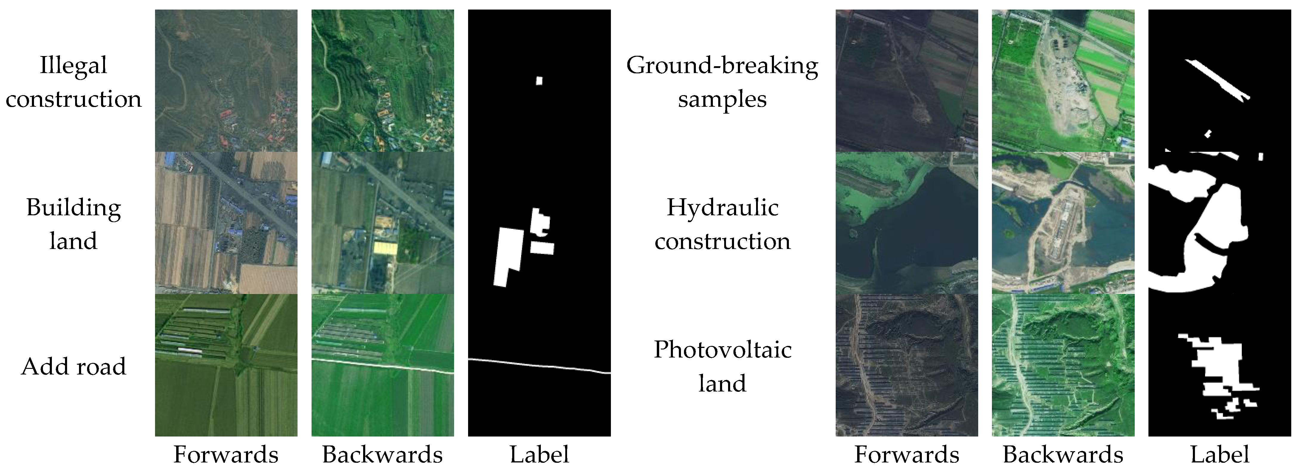
The dataset was in TIF format, and the real values were vector data. Therefore, the rasterization operation was applied to process the vector data into a single-band true label, which was then processed into a recognizable format by using the tool embedded in raster in ArcGIS. Figure 3 shows some newly added construction land information labels. The newly added construction land in Figure 3 includes newly added construction land, new land for roads, illegal expansion of building land, new hydraulic construction land, new ground-breaking land and new photovoltaic land. In each real label, the white area represents the changed area, and the black area represents the unchanged area. In the experimental dataset, images were cut out, and samples of newly added construction land were selected from high-resolution images combined with survey data of land use change as the dataset. After removing the original data, 4328 images were produced, with a size of 512 × 512 each. The dataset was divided into a training dataset and a test dataset with a proportion slightly greater than 9:1. The test data exceeded 10% of the total sample [32], which met the required sample selection proportion.

In the dataset of this study, there are fewer road samples and smaller changing features. Although the number of building land samples is large, some areas with small changes in the characteristics of building land are not easy to be identified. To prevent underfitting due to the small amount of data and enhance the generalization ability of the model, in this study, a series of operations, including translation and rotation [33], were applied to the road samples and construction land samples. The newly added dataset contained 5394 images, while the sample expansion operation was not applied to either the training or test dataset. The expanded training dataset is shown in Figure 4.

6. Parameter Determination of the Focal Loss Function and Analysis of Experimental Result

6.1. Parameter Determination of Focal Loss Function

6.1.1. Determination of the Parameter α

In this paper, the balance factor and limiting factor of the focus loss function are used to balance the weight of positive and negative samples. For positive samples, negative samples with prediction accuracy above 0.95 have little effect on the loss value of the loss function, while negative samples with prediction accuracy below 0.3 have relatively large loss value. For negative samples, a 0.1 forecast must have a much smaller sample loss than a 0.8 forecast. When the prediction result is 0.5, the loss value is only reduced by 0.25 times, which will make the network pay more attention to the distinction of this positive sample, thus reducing the impact of negative samples. This method can be applied to all samples, which not only solves the time-consuming and laborious problem of screening samples, but also ensures the spatial range of the original samples and the feature expression ability of the model.

This experiment used TensorFlow 1.12.0 as the development framework, and the computer hardware configuration was an Nvidia Titan Xp (12 G). The network training took approximately 28 h. The training accuracy rate on the dataset created in this article was 99.7%. To explore the optimal parameters of the FL function for the extraction of newly added construction land information, four models were trained. The parameter settings and specific accuracy evaluations are shown in

Table 1. The value of α when γ = 2.

Focal Loss Function Parameter Setting	Change Area F1-Score	Unchanged Area F1-Score	Kappa
α = 0.1	0.895	0.993	0.897
α = 0.2	0.900	0.993	0.902
α = 0.25	0.871	0.992	0.869

.

In [27], the α parameter was concluded to be one that controls the sample weight. As α decreases, the weight of each negative sample decreases accordingly within a relatively stable range. The two parameters α and γ affect each other and must be selected at the same time. Generally, owing to the relationship between the two parameters, when α increases slightly, γ also increases (in [27], the experiments with α = 0.25 and γ = 2 had the best effect). Therefore, this study first defined the value of the parameter α when γ = 2. From the above accuracy evaluation, when γ = 2, the F1-score and Kappa coefficient of the change area increase with decreasing α.

Because α controls the proportion of positive to negative samples, the value of α is the ratio of the total number of pixels in the positive samples of the training dataset to the total number of pixels in the negative samples. To verify this conclusion, this study further conducted verification experiments. The ratio of the number of positive to negative total pixels in this experimental training dataset was approximately equal to 0.05. To investigate whether α = 0.05 and γ = 2 are the optimal solutions, three models of α = 0.04, 0.05, and 0.06 were selected to verify the experiment. The specific accuracy evaluation is shown in

Table 2. Accuracy evaluation of the α model for determining parameters.

Focal Loss Function Parameter Setting	Change Area F1-Score	Unchanged Area F1-Score	Kappa
α = 0.04	0.885	0.995	0.888
α = 0.05	0.912	0.996	0.913
α = 0.06	0.885	0.995	0.888

.

From the accuracy evaluation in Table 2, when α = 0.04 and α = 0.06, the F1-scores of the two model change regions are almost the same as the Kappa coefficient. When α = 0.05 and γ = 2, the F1-score and Kappa coefficient of the change area reach the maximum value of the interval, indicating that α = 0.05 and γ = 2 yield the best result in this interval. However, since the two parameters are not independent of each other, the value of α needs to be controlled to determine the value of γ.

6.1.2. Determination of the Parameter γ

Because the parameters α and γ are not independent of each other, the two parameters need to be selected at the same time. Therefore, this study chooses to train the model for when (1) α = 0.05, γ = 1; (2) α = 0.05, γ = 2; (3) α = 0.05, γ = 3; (4) α = 0.05, γ = 5; (5) α = 0.05, γ = 1; and (6) α = 0.1, γ = 3. The specific accuracy evaluation is shown in

Table 3. Accuracy evaluation of the γ model for determining parameters.

Focal Loss Function Parameter Settings	Change Area F1-Score	Unchanged Area F1-Score	Kappa
α = 0.05, γ = 1	0.774	0.993	0.761
α = 0.05, γ = 2	0.912	0.996	0.913
α = 0.05, γ = 3	0.881	0.992	0.882

.

From the above table, when α = 0.05 and γ ≥ 2, the value of the F1-score and the Kappa coefficient of the change area decrease as γ increases. Therefore, when α = 0.05 and γ = 2, the F1-score and Kappa coefficient of the change area are the highest. Considering that α also increases with increasing γ, to determine the optimal parameters, the values of α and γ were increased to 0.1 and 3, respectively, at the same time in this experiment.

As indicated in the above table, the F1-score and Kappa coefficient of the model change area with α = 0.1 and γ = 3 were both 0.01 higher than the highest F1-score and Kappa coefficient of other parameters but decreased by 0.11 and 0.10 compared with the optimal parameters. Therefore, the network model has the highest accuracy when α = 0.05 and γ = 2. However, since these two parameters are the optimal solutions for a validation set, to explore their applicability, four independent validation sets were also adopted in this study to verify the applicability of the parameter.

6.2. Experimental Data Analysis

6.2.1. Research on the Applicability of the Focal Loss Function

In this study, four independent validation sets, i.e., validation set 1, validation set 2, validation set 3, and validation set 4, were used for accuracy validation. The specific verification results are shown in

Table 4. Parameter setting and accuracy evaluation.

Focal Loss Function Parameter Setting	Validation Set 1		Validation Set 2		Validation Set 3		Validation Set 4
	F1-Score	Kappa	F1-Score	Kappa	F1-Score	Kappa	F1-Score	Kappa
α = 0.1, γ = 2	0.930	0.939	0.786	0.770	0.800	0.787	0.906	0.904
α = 0.2, γ = 2	0.944	0.935	0.801	0.784	0.791	0.778	0.932	0.926
α = 0.25, γ = 2	0.935	0.923	0.820	0.804	0.719	0.706	0.893	0.886
α = 0.3, γ = 2	0.905	0.892	0.777	0.759	0.748	0.736	0.870	0.862
α = 0.04, γ = 2	0.943	0.944	0.818	0.800	0.764	0.743	0.922	0.912
α = 0.05, γ = 2	0.962	0.952	0.829	0.814	0.806	0.794	0.944	0.940
α = 0.06, γ = 2	0.951	0.93	0.809	0.791	0.768	0.749	0.915	0.900
α = 0.05, γ = 1	0.827	0.812	0.705	0.684	0.671	0.663	0.793	0.777
α = 0.05, γ = 3	0.934	0.922	0.809	0.789	0.783	0.769	0.900	0.893
α = 0.05, γ = 5	0.923	0.909	0.780	0.760	0.772	0.757	0.891	0.883
α = 0.1, γ = 3	0.940	0.941	0.804	0.794	0.786	0.780	0.935	0.928

.

As shown in the above table and the experimental results, the highest accuracies are reached in all verification sets when α = 0.05 and γ = 2. Therefore, the ratio of the total number of pixels of the positive samples to the total number of pixels of the negative samples in the training dataset can be taken as the value of α. Since the value of α in this experiment is 0.05, the value of γ also decreases as α decreases. Therefore, the value of γ in these experimental data is 2. The formula for determining α is shown in Formula (6):

$$\alpha =({\displaystyle \sum _{i=0,j=0}^{m,n}{P}_{i,j}^w})/({\displaystyle \sum _{i=0,j=0}^{m,n}{P}_{i,j}^b})$$

(6)

where m and n are the length and width of the image, i and j are the pixels of the (i, j) sample, p^w is a positive sample pixel, and p^b is a negative sample pixel. Regression analysis of the influence of parameters α and γ on the precision.

Formula (6) is not supported by the corresponding mathematical theory. Thus, regression analysis of the parameters α and γ on the four verification sets and of the extraction accuracy is conducted below, and the curve diagram used to fit the values and accuracy of the two parameters are shown in Figure 5, Figure 6, Figure 7 and Figure 8.

From the above Figure, a higher brightness of yellow means a higher accuracy. In verification sets 1, 3 and 4, the yellow highlights are concentrated within 0 < α < 0.1 and 1 < γ < 3, which shows that the two parameters have the highest accuracy within these two intervals. In verification set 2, the yellow highlights are concentrated within 0 < α < 0.1, 1 < γ < 3 and 0.2 < α < 0.3, 1 < γ < 3. However, from Table 4, when 0 < α < 0.1 and 1 < γ < 3, the F1-score and Kappa coefficient are both higher than 0.2 < α < 0.4.

From the trend of accuracy change in the above Figs., the two parameters are not linearly related to accuracy. Therefore, the regression algorithm uses multiple logistic regression analysis. In this multiple regression analysis, parameters α and γ are independent variables, and the F1-score and Kappa coefficient are dependent variables. The specific analysis results are shown in

Table 5. Multivariate logistic regression analysis of two parameters and their accuracy on the four verification sets.

Parameter	Model Fitting Information (Sig)	Goodness of Fit (Sig)		Pseudo R-Squared			Likelihood Ratio Test (Sig)
		Pearson	Deviation	Cox	Negorco	McFadden	α	γ
F1-score of verification set 1	0.000	1.000	1.000	0.992	1.000	1.000	0.001	0.179
Kappa of verification set 1	0.000	1.000	1.000	0.992	1.000	1.000	0.001	0.179
F1-score of verification set 2	0.000	1.000	1.000	0.992	1.000	1.000	0.001	0.179
Kappa of verification set 2	0.000	1.000	1.000	0.992	1.000	1.000	0.001	0.179
F1-score of verification set 3	0.000	1.000	1.000	0.992	1.000	1.000	0.001	0.179
Kappa of verification set 3	0.000	1.000	1.000	0.992	1.000	1.000	0.001	0.179
F1-score of verification set 4	0.000	1.000	1.000	0.992	1.000	1.000	0.001	0.179
Kappa of verification set 4	0.000	1.000	1.000	0.992	1.000	1.000	0.001	0.179

.

From the above table, the F1-score of the four verification sets and the Kappa coefficient in multivariate logistics regression, the values of the model fitting information (significance), goodness of fit (significance), camouflage R-squared and likelihood ratio test (significance) are all equal because the results extracted on the four verification sets are all extracted under the same model. The statistical meanings represented by the values of each parameter are analyzed in detail below.

(1)

Model fitting information (Sig)

First, the values of the model fitting information (significance) are all 0. The significance judgement condition is that the significance value is less than 0.05, which means that the model is statistically meaningful and has passed the test;

(2)

Goodness of fit (Sig)

Second, the Pearson chi-square and deviation in the significance of goodness of fit are closer to 1, which indicates that the original hypothetical model can fit the data well, with a high probability. Thus, the original hypothesis is valid, and the model fits the original data well;

(3)

Pseudo R-squared

The closer the values of the three pseudo R-squares are to 1, the better the fit of the model. The Cox value of the pseudo R-squared in this chapter is 0.992, and the values of Negorco and McFadden are both 1. Thus, the model can explain the variation in the original variables very well, and the fit is very good;

(4)

Likelihood ratio test (Sig)

In the likelihood ratio test, the significance of α is 0.001 < 0.05, and the significance of γ is 0.179 > 0.05, indicating that α has a significant effect on the construction of the model. Because of the mathematical formula for the value of α in this chapter, the significance value of α above also shows that it is of mathematical significance to study the value of α in this model.

By comparing the precision of the training model after each parameter is selected and through regression analysis of the precision, this study concludes that studying the value formula of α is of mathematical significance and that the original hypothesis model holds.

6.2.2. Comparative Analysis of Experiments

In this study, the U-net, improved U-net, and improved U-Net with the FL function were compared for accuracy analysis. The analysis results are shown in

Table 6. Accuracy evaluation of different networks.

Network Model Category	U-Net		Improved U-Net		Method of This Article
	F1-Sorce	Kappa	F1-Score	Kappa	F1-Sorce	Kappa
Change area	0.834	0.845	0.879	0.887	0.912	0.913
Unchanged area	0.971		0.991		0.996

.

From the table, the F1 score of the method in this paper is improved by 0.05 compared with the unchanged area of the U-net. For sensitive change regions, the F1-score is increased by 0.078, and the Kappa coefficient is increased by 0.068. Compared with the improved U-net (where the loss function is the cross-entropy loss function), the F1-score of the unchanged region is increased by 0.05. For sensitive change areas, the F1-score is increased by 0.033, and the Kappa coefficient is increased by 0.026. According to the provision of the score rate of the Kappa coefficient, a Kappa coefficient greater than 0.8 means that the classification effect is almost consistent. The Kappa coefficient of this research reaches 0.913, which explicitly indicates its feasibility. However, due to the limitation of computer performance, the edge segmentation still needs to be strengthened. Some results of the newly added construction land information extraction are presented in Figure 9.

The Figure above reveals that the U-net does not perform effectively on the bridge samples. It shows a weak ability to recognize false changes in space, and the results of edge segmentation on the building samples are relatively poor. On the other hand, the improved U-net produces better extraction accuracy on the samples depicting moving ground, buildings, bridges, and photovoltaic land but exhibits deficiencies in the extraction of details in some changing areas. Additionally, the improved U-net lacks integrity in the overall patch extraction, leaving vacant parts on the large patch. Compared with the former two methods, this method demonstrates an improved ability to identify spurious changes in space due to the use of the FL function and the weight of the positive sample, making the neural network focus on the positive sample.

In conclusion, the effect of the method for extracting information related to newly added construction land is the closest to the real label, and its segmentation details are more complete. The U-net uses a deconvolution operation during up-sampling. The reduction in the receptive field leads to insufficient feature extraction capabilities and the inability to identify false changes in the Figure. Although the improved U-net could extract the change pattern, the overall performance is unsatisfactory. In the improved U-net, the traditional cross-entropy loss function is introduced, which gives the same weight to the positive and negative samples. However, when newly added construction land information extraction is performed by using the improved U-net, the proportion of positive to negative samples is seriously unbalanced, resulting in a poor overall integrity of the extracted information. In fact, the method proposed in this paper uses the FL function in reference target detection, which also has the problem of imbalance between positive and negative samples. Therefore, a change detection method in the field of remote sensing is introduced in this paper. The experimental results show that applying the FL function to change detection yields a satisfactory extraction effect.

7. Concluding Remarks

This paper proposed a series of improvements to prevent the U-net from overfitting and to address the inability to adequately detail newly built construction land in the U-net. To resolve the imbalance of positive and negative samples in the information extraction of newly added construction land, a FL function was introduced to adjust the weighting of positive and negative samples. The experimental results show that compared with those of the U-net, the F1-score and Kappa coefficient of the change area produced by the proposed method increase by 0.078 and 0.068, respectively, and increase by 0.033 and 0.026, respectively, compared with those of the improved U-net. This proposed method demonstrates the great advantage of newly added construction land information extraction and provides a practical reference for determining the parameter α by using a FL function in the field of deep learning change detection. In addition, this method has significant advantages in extracting information related to newly added construction land and has great application potential for future work

Although the newly added construction land extraction method proposed in this paper has achieved good results in F1 value, the training time becomes longer due to the addition of many improved algorithms. Later, consider how to reduce the time of network training without changing the performance of the model. In addition, because the dataset used in this paper does not include all types of newly added construction land, the classification accuracy of validation set 2 and validation set 3 is slightly lower than the other two validation sets when the accuracy of the four independent validation sets is verified. In the later work, all the data of newly added construction land types are considered to be constructed into a new dataset, and the original network model is fully trained by transfer learning to identify more newly added construction land types, so as to improve the extraction accuracy of the model.

In addition to the above discussion, the focus of this paper is to explore how to reduce the weight of negative samples by controlling the parameter α, so as to improve the information of newly added construction land after the focal loss function is used in U-net network. Since this research is based on U-net as the basic framework, our main purpose is to explore the correctness of our determination and analysis of the parameter α and play a positive role in the semantic segmentation of the improved U-net network, so we take the U-net network and the improved U-net network as the comparison experimental group. We consider it to verify the effectiveness and advancement of our proposed method under the condition of controlling the basic framework. Based on the above considerations, we did not compare the method proposed in this paper with other network models, and the purpose of this is to illustrate the feasibility of the method proposed in this paper as much as possible. Although this practice reflects the correctness of our method well, it lacks comparison with other network models, which causes certain limitations. Therefore, in the future research, our focus will be on a more comprehensive and detailed comparative analysis of the proposed method by using different models and different improved category imbalance methods, including extraction speed, extraction accuracy, model practicability, and model structure complexity. At the same time, more types of data will be segmented extraction verification, not just limited to a limited type of data, as these are essential and necessary.