Stereoscopic Projection Policy Optimization Method Based on Deep Reinforcement Learning

Abstract

Based on the good performance of deep reinforcement learning (DRL) in policy optimization, a stereoscopic projection policy optimization method is proposed, which combines the simulation experiment method with the DRL method. On the basis of policy optimization research, a deep learning framework is selected according to the research problems, and a DRL stereoscopic project policy model based on the asynchronous advantage actor–critic (A3C) algorithm, which uses two groups of neural networks, is constructed. The optimized stereoscopic projection policy is obtained by the interactive learning between the DRL model and the simulation. The effectiveness of the cooperative optimization policy between the DRL and the simulation experiment is verified.

1. Introduction

The uncertainty, antagonism, and emergence of complex operational systems are becoming prominent, which has brought unprecedented technical challenges to the analysis and optimization of operational policy under incomplete information [1]. It is mainly reflected as follows: Firstly, it is difficult to form an effective mapping between decision-making behavior and benefit, and the traditional theoretical analysis and analytical calculation cannot be adopted. Secondly, it takes a long time to reflect the benefits of decision-making, and the lag of feedback affects the overall optimization of policy exploration [2,3,4].

The decision-making process of operations can be regarded as the Markov decision process (MDP); that is, the operations in the current stage will affect the situation in the next stage [2], and the situation in the next stage will affect the action policy. So, many researchers have begun to use the deep reinforcement learning (DRL) algorithm, which is suitable for processing the Markov decision process to study the policy optimization of operations. For example, Yao discussed the possibility of applying the deep reinforcement learning framework to combat mission planning [5]. Wu studied the intelligent simulation platform based on deep reinforcement learning technology [6]. Yu studied the application of hierarchical reinforcement learning in joint operational simulation [7]. Ding studied the method of cooperative operation using RL in the naval warfare environment [8]. Some of the above projects only focus on a type of specific equipment, but fail to take into account the overall situation and complexity, and others focus on conceptual algorithms, fail to combine with typical operational scenarios effectively, and lack military practical significance.

To solve the above problems, this paper proposes a collaborative optimization policy method of stereoscopic projection operations based on a DRL framework and simulation experiment. Firstly, a deep learning framework is selected according to the research problems, and a DRL multi-dimensional strategy model based on the A3C algorithm [9] is constructed. Secondly, the autonomous evolution and capability improvement of policy are realized by the distributed interaction between the DRL model and the simulation. Finally, the decision-making model of stereoscopic projection is obtained, and the global approximate optimal operation policy is obtained.

2. Selection of DRL Framework

Reinforcement learning (RL) is an important branch of machine learning, which is used to describe and solve the problem that agents achieve the maximum reward or achieve specific goals through learning policy in the process of interaction with the environment. According to the given conditions, RL can be divided into model-based and model-free. According to the algorithms used to solve RL problems, it can be divided into on-policy and off-policy. According to the center of optimization, it can be divided into policy-based and value-based. In addition, there is a critic–actor method that combines the advantages of both methods. According to the update frequency, it can be divided into temporal-difference update (TD) and episodic update. In addition, the DL model can be applied to RL to fit the value function, thus forming the deep Q-network (DQN) [10]. The above methods have their own characteristics and need to be selected according to different research problems. The following will combine the actual problem of optimization of stereoscopic projection policy and the characteristics of various RL methods to build a DRL framework that meets the research needs.

2.1. Selection of Model-Based RL and Model-Free RL

Model refers to the environment in RL. It is generally believed that in model-based RL, the transfer function is known, while in model-free RL, the transfer function is unknown. Generally speaking, the learning efficiency of the model-based method is higher, but in practical applications, it is less able to obtain accurate and concise fitting models, so the model-free method is more common in practical applications.

In the process of our work, although the whole stereoscopic projection simulation process can be regarded as a model, it is difficult to obtain this fitting model, and the calculation speed is slower than the learning speed of RL. Therefore, the model-free RL method is chosen.

2.2. Selection of On-Policy and Off-Policy

On-policy means learning and making decisions at the same time. The generated sample policy and learning policy are the same, and the learners and decision makers are the same. The typical algorithms are state–action–reward–state–action SARAS), Epsilon–Greedy, and so on [11]. The advantage of this method is learning speed, and the disadvantage is that it may not be able to find the global optimal strategy.

Off-policy refers to learning through previous historical policy. Learners and decision makers do not need to be the same. The typical algorithm is Q-learning [12]. This method is intended to explore. Its advantages are more powerful and universal, while its disadvantages are twists and turns and slow convergence.

Considering that different policy learning can optimize policy while exploring new policy to collect data, and can start multiple simulators to drive parallel learning tasks, it can meet the requirements of slow simulation speed and distributed parallel operation in the optimization of stereoscopic projection policy, so off-policy learning method is used in the work.

2.3. Selection of Episodic Update and Temporal-Difference Update

A round usually contains many time steps. After a complete round, the policy is modified according to the total rewards obtained by the reward function, which is called the temporal-difference update method. The logic of this method is simple, but the disadvantage is that it cannot be corrected before the end of the round, which means that even if we know that the current action is not the optimal one, we have to wait until the end of the round to correct it.

On the contrary, the method of correcting according to the predicted value after each action is called the temporal-difference update method, such as temporal-difference (TD) learning [13]. This method does not need to wait until the end and can be modified according to the estimated value of the current state and strategy. Because this method is based on the current estimated value, not necessarily the real reward value, the accuracy of the correction is insufficient.

This work uses simulation and DRL framework for distributed interactive learning. Therefore, the multi-step learning method between the two, which can take into account the actual reward value and certain multi-step prediction ability, is selected to build the RL framework.

2.4. Selection of Value-Based RL and Policy-Based RL

In RL, the value function is a function to measure the degree of good state according to the prediction of future reward value. There are two common expressions.

One is the state value function $V^{\pi }\left(s\right)$, which represents the expected total value obtained by taking the policy in the initial state s, expressed as Formula (1) [11] as follows:

$$V^{\pi }\left(s\right)=E_{\pi }\left[R_t|s_t=s\right]=E_{\pi }\left[{{\displaystyle \sum }}_{k=0}^{\infty }{\gamma }^k{r}_{t+k+1}|s_t=s\right]$$

(1)

The other is the action value function $Q^{\pi }\left(s,a\right)$, which represents the expected total value obtained by taking action $a$ in state $s$ and subsequent actions complying with the policy, expressed as Formula (2) [12] as follows:

$$Q^{\pi }\left(s,a\right)=E_{\pi }\left[R_t|s_t=s,a_t=a\right]=E_{\pi }\left[{{\displaystyle \sum }}_{k=0}^{\infty }{\gamma }^k{r}_{t+k+1}|s_t=s,a_t=a\right]$$

(2)

The policy π is a probability distribution, which reflects the probability of selecting actions in a certain state.

$${\pi }_{\theta }\left(s,a\right)=P(a|s,\theta )$$

(3)

The θ in Formula (3) is the parameter in the policy function.

In model-free RL, it is usually difficult to directly obtain an accurate value function, so it is necessary to use a value function approximation instead.

The purpose of value-based RL is to learn the approximate function of value, make it conform to the actual reward, and generate the best strategy. Policy-based RL aims to use parametric functions to learn policy functions directly without calculating the value function.

The two methods have their own advantages and disadvantages. The value-based method must choose the action that maximizes the value function. If the action space is very high-dimensional or continuous, the cost will be high, while the policy-based method operates by adjusting the parameters of the policy directly, and does not need to maximize the calculation. Therefore, the policy-based method is more stable, and can learn both deterministic and stochastic policy. However, compared with the value-based method, the policy-based method is slower, and converges to the local optimal rather than the global optimal.

To combine the advantages of the above two, the popular method is to use the critic–actor algorithm, which is an RL method combining policy gradient and time-series differential learning. Actor refers to the policy function ${\pi }_{\theta }\left(s,a\right)$, that is, learning a policy to get the highest reward. Critic refers to the value function $V^{\pi }\left(s\right)$, which estimates the value function of the current policy.

With the help of the value function, the critic–actor algorithm can update the parameters in one or more steps without waiting until the end of the whole round. In each step, the policy function and value function are trained respectively. At the beginning of the learning, the actor executes the policy and the critical evaluates randomly. Through continuous learning, critical evaluation is more accurate, and policy is better.

In the work, the critic–actor algorithm will be used to construct the RL framework.

2.5. DRL

Due to the explosion of state spaces and action spaces [11], traditional RL methods will be limited by the curse of dimensionality. Therefore, the universal approximation characteristics of neural networks can be used to fit the value approximation function and policy function. If deep neural networks such as long short-term memory (LSTM) network or convolutional neural network (CNN) are used, the deep reinforcement learning framework can be obtained. Typical algorithms include deep deterministic policy gradient (DDPG) [14], advantage actor–critic (A2C), asynchronous advantage actor–critic (A3C), proximal policy optimization (PPO) [15], etc.

DDPG is an algorithm that uses a neural network to output a deterministic action and can be used in continuous action space. It is also a temporal-difference update policy network, which trains a deterministic policy through off-policy. Because the policy is certain at the beginning, it may not be able to try enough actions to find useful learning signals. In order to explore DDPG’s policy better, it is necessary to add noise to action during training. The original author of DDPG recommended using time-related Ou noise, but using this method with many super parameters to explore the environment is slow and unstable [14].

PPO is an off-policy gradient algorithm. It is usually sensitive to step size, and it is difficult to select the appropriate step size. If the difference between the old and new strategies is too large in the training process, it is not conducive to learning. PPO proposes a new objective function, which can add a training step to achieve small batch updates, and solves the problem that it is difficult to determine the step size in the policy gradient algorithm. Its advantages are stable training, simple parameter adjustment, and strong robustness [15].

The A2C algorithm, which uses the advantage function to replace the original return in the critic network, can be used as an indicator to measure the quality of the selected action and the average expectation of all actions. In Formula (4), it shows that the dominant function $A^{\pi }\left(s,a\right)$ is the difference between the state function and the state-action function. If the function is greater than zero, it means that the action is better than the average action; otherwise, it means that it is worse than the average action.

$$A^{\pi }\left(s,a\right)=Q^{\pi }\left(s,a\right)-V^{\pi }\left(s\right)$$

(4)

The A2C algorithm uses synchronous update to learn, which has low learning efficiency. In order to improve the learning efficiency, the A3C algorithm was chosen. Asynchronous means to open multiple actors to explore the environment and update asynchronously. This method means that the data are not generated at the same time, and multiple threads can be used. Each thread is equivalent to an agent exploring randomly, and multiple agents exploring together, parallel computing policy gradient, and maintaining a total amount of updates [9].

Because of the higher learning efficiency of the A3C algorithm [16], it will be used as the RL framework in our work.

3. Construction of Stereoscopic Projection Policy Model Based on DRL

3.1. Operational Concept

During the operations, the red’s purpose is to suppress the blue side with firepower as soon as possible, and use plane, air, surpassing, and other projection methods to send troops to the land of the blue side comprehensively.

In the whole process, the damage should be as small as possible, and the success rate of projection should be as high as possible. At the same time, the land forces can complete the fixed mission within a certain time.

The forces of red can be divided into three categories roughly: combat forces, support forces, and projection forces.

(1) Combat forces: These are mainly responsible for damaging the effective power of the other side directly. Air-based air-to-air power mainly refers to an air-superiority fighter and is mainly responsible for air-to-air tasks. Air-based ground/sea forces include armed helicopters, fighter planes, bombers, etc., which are mainly responsible for ground-to-sea bombing missions. Sea-based forces include frigates and destroyers, taking into account air defense and shore-to-shore artillery missions. Land-based air/ground forces include cruise missiles, long-range firepower, air defense missile positions, etc., which are mainly responsible for key ground attack and near-shore air defense.

(2) Support forces: These mainly include three categories: land-based electromagnetic, air-based electromagnetic, and sea-based obstacle removal. Land-based electromagnetic is mainly a fixed radar station. Air-based electromagnetic includes electronic reconnaissance aircraft, early warning aircraft, electronic warfare jammers, etc., and sea-based obstacle removal is mainly minesweepers and engineer ships.

(3) Projection forces: These mainly include a variety of equipment platforms that can perform landing operations, such as amphibious landing ships, transport helicopters, etc., which can be used to project landing forces.

The military strength of the blue is roughly the same as that of the red side, but its task is to refuse and fight against landing. Therefore, there are no ship forces, but a large number of sea-based obstacles are deployed at key ports, such as mines and other landing obstacles. There is no projection force, but a large number of mobile troops are deployed on the land, such as infantry, self-propelled artillery, tanks, mobile air defense positions, etc., mainly responsible for countering the red army land force.

3.2. State Space

The above concept involves many factors. If a set of state parameters is designed for each related factor, it will fall into the problem of dimension explosion. Therefore, it is necessary to sort the importance of relevant factors and ignore some secondary factors.

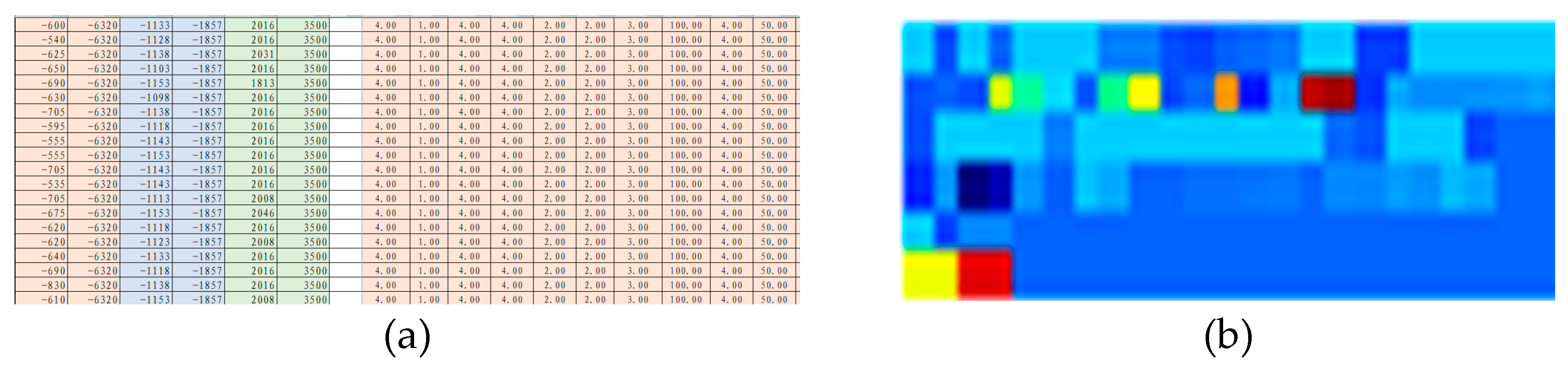
This paper focuses on the research of delivery policy, such as delivery mode, delivery time sequence, delivery capacity, etc. Sensitivity analysis is carried out through pre-simulation experiments to screen the state space. A total of 1 baseline scenario and 17 experimental scenarios were set for pre-experiment. Based on the deduction mode of “out of the loop”, 540 simulations were run, and 23,400 data samples were obtained (partly in Figure 1a below). The character choice results of 18 simulation pre-experiments are shown in Figure 1b as a heatmap.

Through sensitivity analysis, the final selected state space is shown in

Table 1. State space tab in each time step1 state space in one time step.

Serial Number	Combat Power	Status Parameters
1	Combat units (except the projection units), 69	Remaining quantity
2	Projection units (except transport helicopter), 3	Remaining quantity, current speed, departure status
3	Transport helicopter units, 3	Remaining quantity, current speed, departure status, current altitude

, focusing on 69 combat units, 3 projection units (except helicopters), 2 shipborne transport helicopter units, and 1 shore-based transport helicopter unit.

In order to facilitate the construction and learning of the DL framework, the state parameters are discretized. For the combat forces, their position, speed, and other attributes are ignored, and only the survival situation is considered; that is, only the remaining quantity of a certain type of equipment in a certain time step is considered. For example, in time step 10, there are 13 A-type armed helicopters left on the red side, so the value of this variable is 13, which is a discrete variable obviously. For the state parameters of the projection force concerned, it is more sufficient to consider, in addition to the remaining quantity, three variables of the speed, altitude (only helicopters), and whether to sail off the platform at the current time are also considered. Speed is also a group of discrete variables. For different types of delivery platforms, they are divided into four states (creeping speed, cruise speed, assault speed, full speed). The altitude mainly considers the ground clearance of the transport helicopter, which is divided into four states (100 m, 200 m, 400 m, 1000 m). Whether to sail indicates whether the delivery platform is dispatched, which is represented by two discrete variables [0, 1]. Here, 0 means it has not been dispatched, and 1 means it is already on the way.

To sum up, there are 75 + 6 + 6 + 3 = 90 state parameters, all of which are discrete parameters.

3.3. Action Space

Our work focuses on the optimization of the stereoscopic projection policy, the operational policy of the combat forces is ignored. For the projection forces, there are two states in each time step, acted and not acted.

To ensure the discretization of action space parameters, the assumptions are made as follows: Firstly, all the projection forces can only perform the projection task once, and there is no return flight to perform the projection task again. Secondly, there is no split problem of the projection force grouping.

Based on the above assumptions, during the transition between the two states of action and inaction, there are three action spaces that can be selected for execution: First, the last time step is not action, which determines whether to act. Second, the last time step did not take action. This time step determines the action. While determining the action, it also determines the unit size, speed, altitude, etc. Third, the unit has been moved in the last time, and the speed and height of the formation can be adjusted by continuing to move in this time step. The formed action decision space is shown in

Table 2. Action space in one time step.

Serial Number	Combat Power	Action Space
1	Inactive projection force	[0, 1] (0 means to hold, 1 means to sail)
2	Projection force without action, but has decided to act within this time step	Scale, quantity, speed, altitude (helicopter)
3	Acting projection force	Speed, altitude (helicopter)

.

3.4. Reward Function

The reward function is a regression formula for obtaining rewards from the state. Reasonable design is the key factor for RL to achieve perfect results. If the design of the reward function is not reasonable, the RL framework may find some meaningless policy.

It is focused on the stereoscopic projection action policy, that is, the size of land forces, formation structure, formation, air–sea ratio, projection method, projection time, etc. Therefore, the reward function mainly focuses on the achievement of the red side’s combat purpose, integrating multiple variables such as the arrival rate, combat loss, and defense time into a scalar, which is calculated in each time step of the simulation scenario. In addition, we should also punish the extra throwing power.

Based on the above analysis, the following definition of reward value is given.

Definition 1.

Record the reward value of t at any time as  $R_t$, then

$$R_t=R_{t-1}+(R_1+R_2+R_3+R_4+R_5|s=s_t)$$

Of which, $R_{t-1}$ represents the reward value of the previous moment:

1. 

$R_1$ is the loss of the red side, that is, the force lost by the red side in a certain simulation time step. This value is negative and is obtained by the accumulation of various specific equipment scores.

2. 

$R_2$ is a one-time reward for the red to land. It is a positive number and is given within the time step of the successful landing. If the projection platform is destroyed in the process of projection, the reward cannot be obtained.

3. 

$R_3$ is the continuous reward for the survival of the red. It is a positive number. Whether the landing troops are alive is checked at each time step after the successful projection. If they are alive, the reward is obtained in this time step.

4. 

$R_4$ is the reward for the red to complete the occupation task. After the end of the last simulation time step, the landing position is checked. If there are red units but no blue units in the position, it will be regarded as a successful occupation, and a positive reward will be given at this time.

5. 

$R_5$ is the reward for the number of delivery platforms of the red, which is a negative number. This value has a negative correlation with the delivery power that has taken action in the current time step; that is, the more the delivery power, the smaller the value, which means more penalty points. Although the more projection platforms, the more land troops will be, it is not consistent with our hope to achieve the combat goal with the minimum transport capacity. Therefore, setting negative feedback of the platform quantity policy in the reward function is to ensure the expected requirements.

According to the above definition, the purpose of policy optimization is to maximize the reward value at the end of the last time step. In this work, a fixed simulation time is used to trigger the end of the simulation. The total simulation time is 6 h, and every 5 min is used as a time step, a total of 72 time steps. At the beginning of each time step, the simulation environment interacts with the DRL environment, outputs the current reward value at the end of each time step, and the final reward value after the end of the last time step.

3.5. Value Function and Policy Function

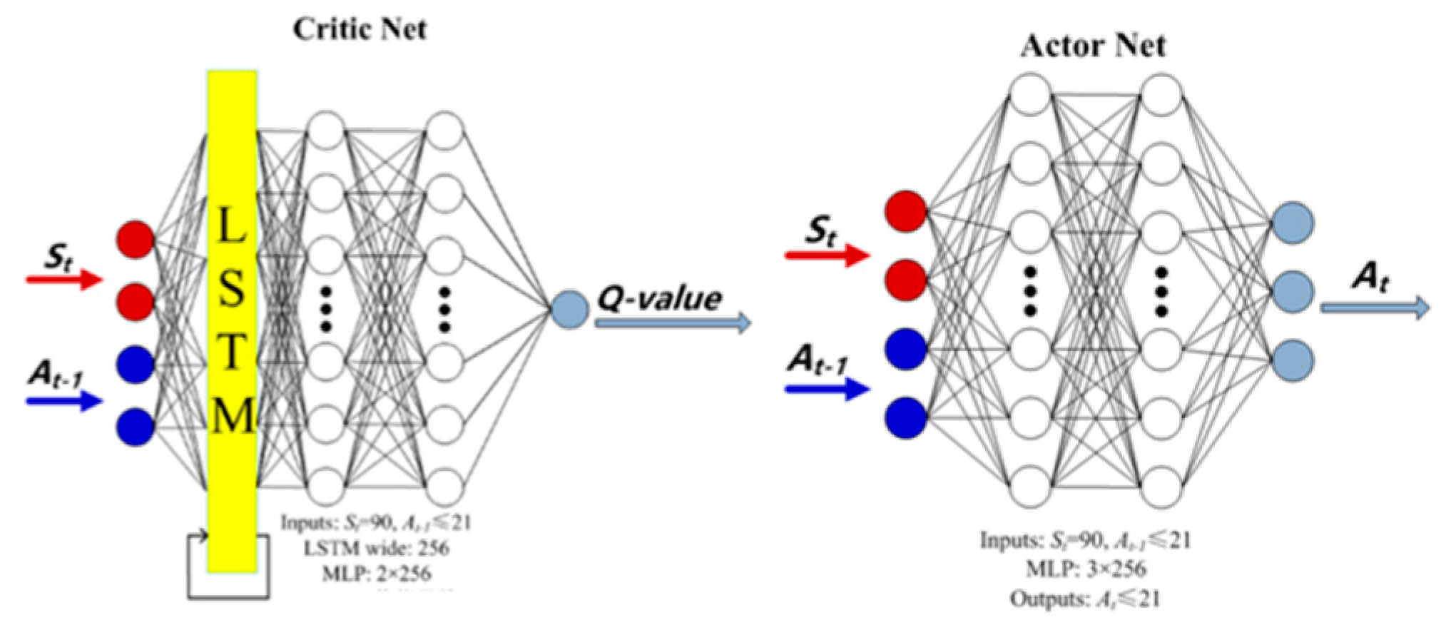
Based on the analysis in the first section, this paper uses the A3C method of off-policy, multi-step learning to build a DL framework. The A3C method is one of critic–actor, which needs to use two groups of neural networks, a critic network and an actor network, to evaluate the value function and policy function. Both groups of neural networks need offline training. As shown in Figure 2.

For critic networks, the input layer is the action instruction of the previous time step (if it is the first time step, the action instruction of the previous time step is regarded as 0), and the state parameters of the current time step. After normalization, it is connected to a hyperbolic tangent activation function, and then connected to a 256-wide LSTM. Because the LSTM neural network is good at dealing with time sequence problems, it is very suitable for MDP problems of the operational sequence. On the one hand, the output of the LSTM is used as its own input, and on the other hand, it is connected with a multi-layer perceptron (MLP), which is good at fitting nonlinear relationships. The multi-layer perceptron has two hidden layers, each layer has 256 neurons, and the exponential linear unit (ELUS) is used as the activation function in each layer to map nonlinear relationships. Finally, a linear layer is used to output the value of the current action, namely the Q value. The ELUS function is shown in Formula (5).

$$\left(x\right)=\{\begin{array}{c}\alpha \left(e^x-1\right) , x\le 0\\ x , x>0\end{array}$$

(5)

α is a super parameter of Formula (5). The convergence rate can be adjusted by adjusting this parameter.

For the actor network, its input layer is the same as the critic network. It is connected to the hidden layer with 256 neurons through a linear layer. The output of the linear layer is normalized and activated by the boundedness of the hyperbolic tangent function, and then sent to the three-layer MLP. The MLP has the same structure as the critic network. The MLP is connected to the output layer through a linear layer. The output layer includes the average value of each action decision and the standard deviation of the corresponding Gaussian distribution. When actually fed back to the model for execution, only the average value of the action decision needs to be executed.

4. Model Training and Experimental Results Analysis

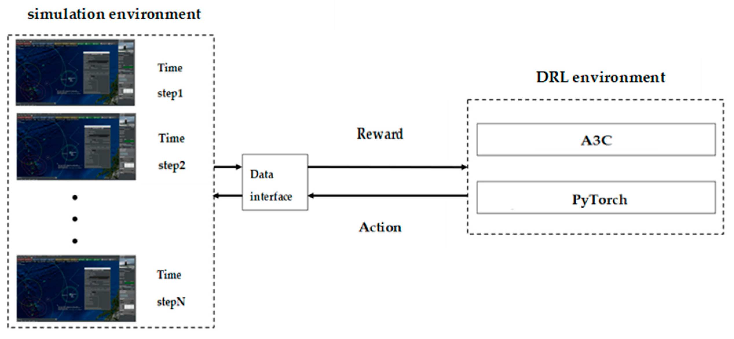
The training environment is shown in Figure 3, which mainly includes three parts:

The first is a visual simulation environment. It mainly relies on an “out-of-the-loop” simulation platform, and the simulation entity implements the deduction according to the preset combat doctrine and scenario running script.

The second is a DRL environment. Based on the PyTorch framework, it is used for agent decision-making learning and implementation.

The third is the interactive data interface. The simulation experiment environment and DRL environment interact offline through the data interface in each time step.

4.1. Model Training Process of Interactive Learning

The running speed of the simulation is much slower than the learning speed of the RL framework. In order to alleviate the problem of relatively little training data, the A3C algorithm is used for asynchronous distributed training to improve the training speed. Each learning model instance running in the tensor process corresponds to 10 critic–actor networks. Each one drives an independent simulation model. A total of 100 simulation models are run in parallel. Each simulation model uses 30 times simulation acceleration. It takes about 0.2 h to run a complete 6 h simulated time.

The training process is realized by the interaction between the simulation model and the RL framework. At each time step, the instructions given by the RL framework are loaded into the simulation model, and the calculation results are given through the simulation model. In the initial stage of training, the action instruction set is loaded into the simulation model according to the diagonal Gaussian distribution, which is to explore as many better instruction sequences in the learning stage.

The learning process is repeated over 72 steps. The learning rate is set to 0.001, the discount rate is set to 0.95, and the batch size is set to 256.

4.2. Analysis of Training Results

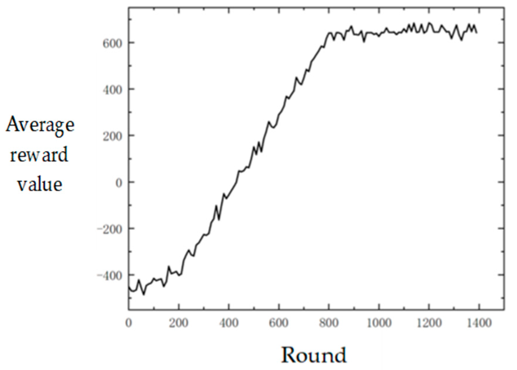
The interactive learning training is carried out according to the above method, and the average reward values are shown in Figure 4.

It can be seen that after 800 rounds of training, the stereoscopic projection policy model based on DRL gradually converged, and the average reward converged to about 635 points. It can be seen from the analysis that in the initial learning stage, that is, the first 200 rounds of training, the policy adopted is inefficient because the action space is explored according to the predetermined initialization policy at this time. For example, the projection platform may directly rush into the blue air defense fire and be destroyed, so the reward score obtained is also low. However, the model will find more efficient strategies soon, and the average reward will rise gradually and converge after 800 rounds of training.

4.3. Optimization Policy Analysis

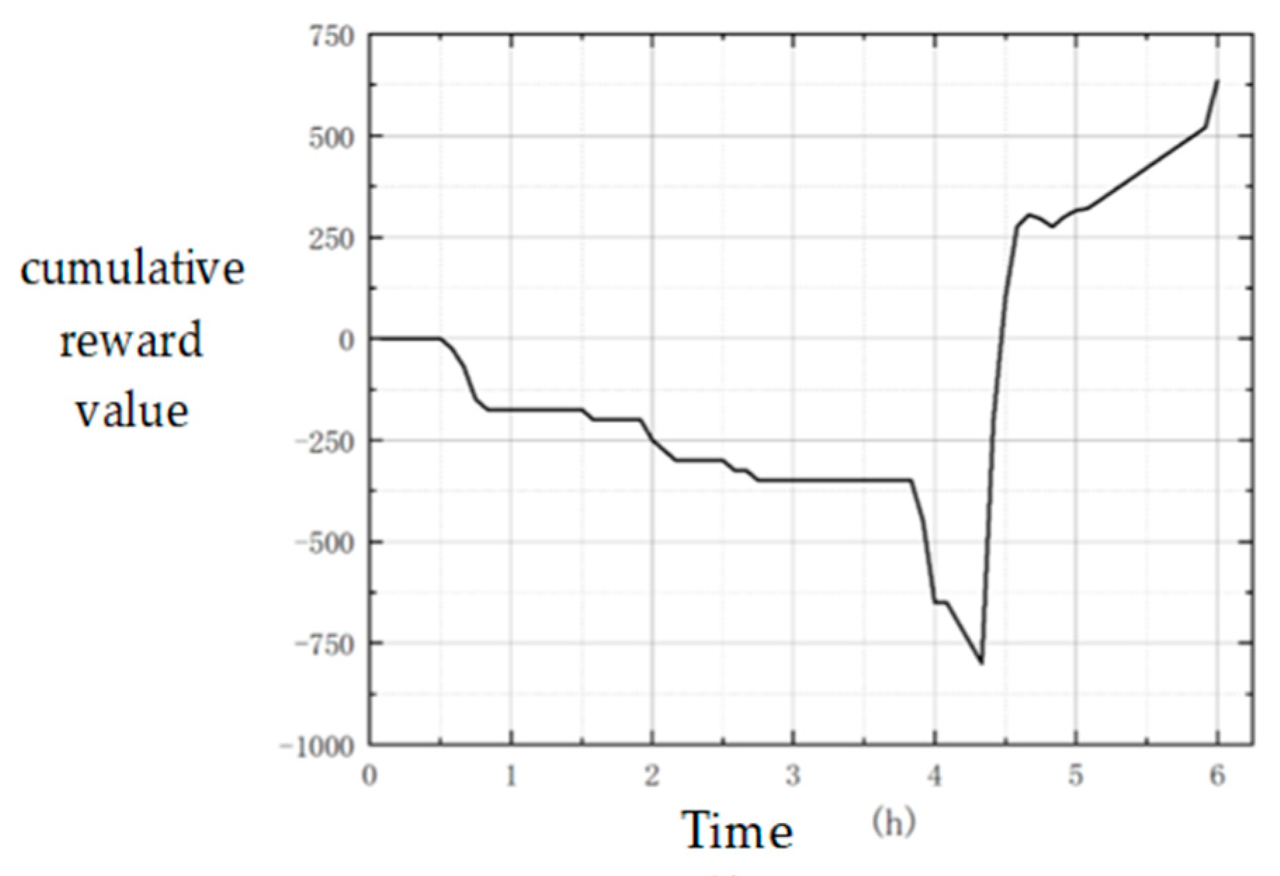
The final optimized policy is used to run the simulation again, and the curve of the cumulative reward value is obtained in each time step, as shown in Figure 5.

It can be seen that, in order to prevent the projection platform from being attacked by the blue superior firepower within three hours at the beginning of the simulation, the red side did not send out the projection platform, but the combat forces carried out the firepower task. Due to the large battle losses caused by the red and blue’s fight for air supremacy, the reward values of the red side were all negative.

In about four hours, the reward value of the red side continued to decrease, because in order to ensure the smooth implementation of the mission, the red side went deep into the blue position to carry out the ground attack, which brought a lot of war damage.

In about 4.5 h, the sea and air delivery platform started to operate and arrived at the blue position almost at the same time. This round of successful landing brought a rapid increase in the reward value of successful delivery $R_2$.

Subsequently, the red landed successfully. With the cooperation of the superior air force of the red, the blue ground army was quickly cleaned up. After five hours, the reward value $R_3$ increased steadily due to the existence of the survival reward, and a large number of rewards for successful occupation $R_4$ were obtained after the last time step.

The overall delivery quantity is constrained by negative feedback $R_5$, and the selected dispatch scale after RL is close to the manual expected value.

4.4. Algorithm Comparison and Analysis

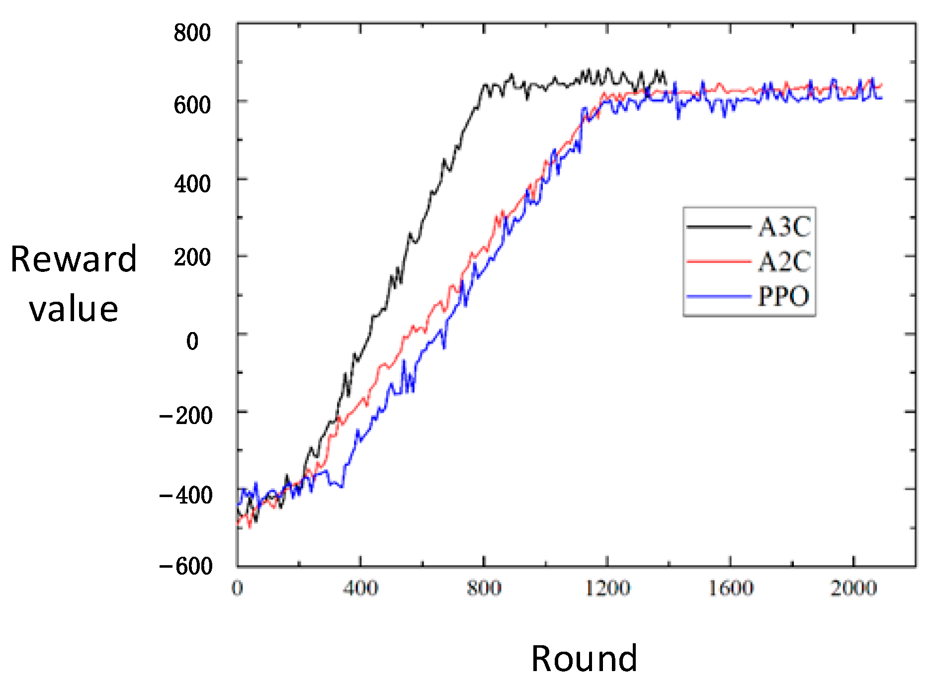
The PPO method and A2C method are used to train the model, and the A3C method constructed in this work is used to conduct a comparative experiment. The relationship between the training rounds and the average reward value is recorded, and the results are shown in Figure 6.

Because the PPO method and the A2C method adopt the policy of synchronous update, they take longer to update than the A3C method of asynchronous update, and the final optimization result is slightly lower. The convergence rate of the PPO method is similar to that of A2C, and the reward value obtained after final convergence fluctuates more, which is related to the super parameter of the proportion of new policy and old policy in the PPO algorithm. If the proportion of the new policy is large, the convergence will be accelerated, but because it tends to choose the new policy with greater benefits and greater risks, the final convergence value will fluctuate greatly. If this ratio is reduced, its convergence speed will slow down.

This experiment results show that the A3C method is better in the field of convergence speed and final optimization results.

5. Conclusions

Taking the stereoscopic projection operation as the main research object, this work proposes a DRL framework and simulation deduction experiment collaborative policy optimization method. In this method, a DRL framework based on the A3C algorithm is constructed, a reasonable reward function is designed, a critic network is constructed by using LSTM and MLP neural networks to calculate the value function, and an actor network for generating action instructions is constructed by using the multi-layer MLP neural network. The DRL model and the simulation of “out of the loop” were interacted in 20 virtual machines. Finally, the optimized stereoscopic projection policy was obtained. The content of the optimized delivery policy is reasonable and in line with expectations, which significantly improves the final reward score, and verifies the effectiveness of the collaborative optimization decision between the DRL framework and the simulation model.

The presented method work can be extended to other cases. This field is still in the initial exploration stage, and the following issues need further research:

(1) Interpretability of DNN.

(2) In order to simplify the calculation process, the designed scenario, action space, state space, and so on have been greatly simplified, and the complexity is still low compared with the real battlefield [17,18].

(3) Although the obtained model performs well in a specific scenario simulation model, it is not necessarily applicable to the same but not identical scenario simulation model; that is, the generalization of the obtained combat policy is insufficient. In the future, transfer learning, meta-learning, and other methods will be adopted to improve it.

(4) Although the model-free RL framework does not need to train label data, it has many problems, such as low training efficiency, poor interpretability, and useless expert experience. In the future, further exploration will be carried out in the field of model-based RL and combination with decision trees and other methods [19].