Speech Emotion Recognition Using Audio Matching

Abstract

It has become popular for people to share their opinions about products on TikTok and YouTube. Automatic sentiment extraction on a particular product can assist users in making buying decisions. For videos in languages such as Spanish, the tone of voice can be used to determine sentiments, since the translation is often unknown. In this paper, we propose a novel algorithm to classify sentiments in speech in the presence of environmental noise. Traditional models rely on pretrained audio feature extractors for humans that do not generalize well across different accents. In this paper, we leverage the vector space of emotional concepts where words with similar meanings often have the same prefix. For example, words starting with ‘con’ or ‘ab’ signify absence and hence negative sentiments. Augmentations are a popular way to amplify the training data during audio classification. However, some augmentations may result in a loss of accuracy. Hence, we propose a new metric based on eigenvalues to select the best augmentations. We evaluate the proposed approach on emotions in YouTube videos and outperform baselines in the range of 10–20%. Each neuron learns words with similar pronunciations and emotions. We also use the model to determine the presence of birds from audio recordings in the city.

1. Introduction

Automatic product recommendation has significant benefits across different business domains [1]. Consumers often refer to YouTube video reviews when making a buying decision [2,3]. The audio signal in a video product review is a good indicator of the polarity of the speaker. For example, a high pitch is often associated with ‘surprise’ or ‘happiness’. In contrast, low frequency tones correspond to ‘sadness’. Predicting the emotional state of a person from their speech is also useful for tele-customer support where physical interactions with the consumers are limited [4].

To enable efficient communication during video meetings over Zoom or Facetime, it is necessary to judge the emotions of a speaker from their voice. In order to maintain the privacy of attendees, we can convert the spoken sounds into a vector representation of floating numbers [5]. The vector representation will allow semantically similar words with similar emotions to be close together in feature space [6]. Another application of predicting emotions from speech is in product recommendations from YouTube videos. The speakers can be from different cultural and language backgrounds. However, the vector representation of sounds will allow training the models in one language and testing in another.

In this paper, we look at two main challenges to detecting emotions from speech. Firstly, the annotation of human speech is very challenging due to differences in pronunciation and level of expression [7]. This could be due to an accent acquired at birth or the use of microtexts in a particular domain [8]. The second challenge lies around data privacy laws, where the use of personal data on social media is now prohibited. To deal with differences in speech among humans, we consider two solutions.

The first is to convert the sound signal to a spectrogram using a Fourier transform [9]. This allows the easy visual comparison of different tones. Figure 1 illustrates the spectrogram for two audio signals from the same speaker and for the same piece of text. The first spectrogram with a low frequency is for happy emotions while the second one with higher frequencies is for anger emotions. We first split each audio into small segments called phonemes. Next, we convert the spectrogram of each phoneme into a vector representation of known human features [10]. The sequence of phonemes is used to train a classifier with memory states for past utterances [11].

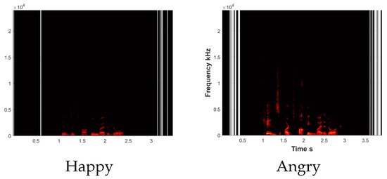
Figure 1. Spectrogram for the same speaker and different emotions. Both utterances are ‘Kids are talking by the door’.

The second solution is to integrate the semantic meaning of spoken words into the classifier. For this, we use concepts with known polarity in a vector space of emotions [12,13]. Negative concepts often begin with prefixes such as ‘con’ or ‘ab’. We use a model trained on spoken concepts as a prior for the real world dataset. Figure 2 illustrates the proposed speech classification framework. Affectivespace is used to initialie the weights of the classifier [14].

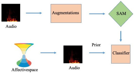
Figure 2. Flowchart of the proposed SAM audio classification model.

Our model will use paired data in the form of voice signals and human annotation to train the model and then discard it from memory. Hence, only the numerical weights of the trained model will be stored without the use of any personal information such as the identity of the consumer [15]. We also propose the use of data augmentation approaches such as modifying the pitch, amplitude or frequency of a speech recording to create additional samples [16]. Speech audio matching (SAM) is used to select the best augmentations with respect to a gold standard audio sample. As such, we can discard samples with high noise that will reduce the accuracy of the classifier. Figure 2 shows that the audio signals are augmented to create a new training set. The proposed SAM is used to select a subset of samples for training the classifier.

The organization of the paper is as follows: Section 2 provides a literature review of articles on emotion prediction from speech and their shortcomings; Section 3 describes the oral cavity transfer function and the use of a sequence model to predict the next sound; Section 4 details the proposed approach to integrate Affectivespace and a new metric for augmenting sounds; finally, in Section 5 we evaluate our approach on the tasks of human emotion classification and bird detection and provide conclusions in Section 6.

2. Related Works and Contributions

Video product reviews are a source of multimodal information in the form of text, audio and images. Some people express their opinions more vocally and others rely on facial expressions [17,18]. Hence, in our previous work, we considered the fusion of the speech and image features using multiple-kernel learning. We observe that accuracy in audio modality is low when using openSMILE features on a binary positive or negative classifier. In contrast, the proposed SAM shows improved prediction on the multi class problem of neutral comments in a Spanish product review [19].

In [20], the authors proposed using correlation to project both audio and video modality into a common space for sentiment prediction [21]. They consider a binary classifier that can predict sentiments from speech using the common vector space. Our approach can work on multi-class emotions and the shape of the oral cavity is robust to fluctuations in sounds for the same emotions. In [22], the authors studied sentiments in tourists as posted on Twitter. They conclude that the length of stay in a location is inversely correlated with the enjoyment level in tweets. Another study showed that unhealthy foods induce a higher level of happiness [23]. The accent of tourists is often distinct from locals, hence prior knowledge of origin can be used to predict the emotion in speech.

Gaussian mixture models (GMM) [24] are popular for the classification of audio signals as they can easily eliminate background noise and other bird sounds in a recording. However, they are unable to model the sequence of phonemes in speech. The long-short-term-memory (LSTM) [16] model can capture variations in long recordings using memory states. In [15], the authors then converted audio recordings into spectrogram images and then classified the images using conventional image processing methods. ‘Yamnet’ is a pretrained deep network that can predict 521 audio events, such as the ’barking of a dog’ [25]. Such an approach will not work with human emotions where there are minor fluctuations in the spectrogram.

In [26], the authors introduced the concept of the alignment of features in the lower and upper layer during the convolution for the RAVDESS speech emotion dataset. They concatenated the outputs of different convolutional kernels and then used a squashing function to obtain a vector representation. Such a model can reduce the information loss during the max pooling of features. However, squashing the output can lead to misalignment. Instead, in this paper, we propose the use of error matching to discard noisy features prior to training.

In [27], audio and visual matching were used to determine the source of sounds in a video. The sound category and the visual appearance are synchronized to identify sounding regions in a self-supervised manner. This approach requires that the object producing the sound is available in the pretrained segmentation model. We overcome this limitation by matching the expected error of generating the audio with a known audio sample from each emotion. In [28], the authors tried to detect the background noise during silent pauses between bird calls. However, the noise profiles will keep changing based on your surroundings. Hence, in this project we aim to integrate prior knowledge of emotions into the prediction.

Lastly, we would like to clarify that transformers are non-sequential models that process the entire input collectively instead of individual phonemes. They are hence effective on short sequences such as in text translation [21]. Speech classification requires us to split each word into phonemes resulting in an extremely long input. Similarly, in this paper, we show that LSTM is superior to recurrent neural networks (RNN) for long-term memory tasks because it does not require additional memory states. To optimize the parameters for the LSTM, previously heuristic-based methods have been used [29]. However, due to the highly non-convex nature of speech manifold, we show that a semi-definite assumption would be able to find the global minima.

We can summarize the main contributions of this paper as follows:

• We propose a metric to match two audio signals that are sensitive to noise.
• We initialize the weights of the model using spoken concepts in a vector space of emotions.
• We show that the SAM metric can select high-quality augmentations and reduce the running time.

Previous authors have proposed a self-supervised model for each species. For example, a dog can be identified by a ‘bark’. However, when detecting different emotions in the same human, we can leverage the pretrained Affectivespace of 24 emotions. Due to a lack of annotated samples, the augmentation of the audio data is performed prior to training a LSTM model. Some of the augmentations have a high level of noise that can reduce accuracy during training. Hence, we propose an audio matching metric using a semi-definite stability constraint that is sensitive to noise.

We show that signals with similar semi-definite solutions have similar noise spectrums. As such, a huge improvement in running time is also achieved. We also consider a self-supervised audio emotion model where speech is mapped to phonetically similar concepts in Affectivespace. During training, mismatched sounds with the same affective regions are suppressed using a supervised sequence model. Both the audio and affective mapping are combined to predict the emotion. To evaluate our model on time series data, we use the Ryerson Audio-Visual Database of Emotional Speech and Song (RAVDESS) [30] speech audio for emotion detection, Multimodal Opinion Utterances Dataset (MOUD) [31], the YouTube product reviews dataset and bird call identification data [32].

3. Preliminaries

In this section, we first explain how the shape of the oral cavity in humans can affect the sound produced during speech. Next, we describe a state space model that can predict the next sound in a sentence based on previous sounds. Lastly, we show how to convert each sound to a vector representation of 39 features commonly observed in human speech.

Notations: Throughout this manuscript, we represent a 2D matrix using upper-case $\mathrm{C}$, a variable using lower-case italic $\beta$, a constant with lower-case $\mathrm{t}$ and a function using lower case with round brackers $f\left(\right)$.

3.1. Oral Cavity Transfer Function

Figure 3a shows that different sounds are produced in the human vocal tract using unique positions of the tongue and other articulators. The vibration of air will result in a particular sound. For example, ’iy’ in the word ’tea’ has a narrow tract and for ’ae’, as in ’cat’, the tract is much larger. Unlike a machine, the human ear perception of sound is non-linear. We tend to be more discriminative at lower frequencies and less discriminative at higher frequencies. The Mel scale can be used to convert the observed sound into what would be heard by the human ear. Depending on the size of the oral cavity, the sounds follow the following transfer function as shown in Figure 3b. The sound signal $x\left(t\right)$ reduces and then increases at the inflection point ${\mathrm{m}}_b$ where it is the lowest in a single phoneme. Then, the slope $h\left(t\right)$ on the left and right for time index t can be given by:

$$h\left(t\right)=\left\{\begin{array}{cc}{h}_r,\hfill & k<{\mathrm{m}}_b.\hfill \\ h_l,\hfill & k\ge {\mathrm{m}}_b\hfill \end{array}\right.$$

(1)

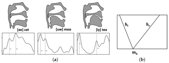
Figure 3. (a) Positions of human vocal tract for different sounds; (b) Transfer function for vocal tract.

Then, we can define the oral cavity transfer function $s\left(x\right(t\left)\right)$ as follows:

$$\begin{array}{ccc}\hfill s\left(x\right(t\left)\right)& =& h\left(t\right)x\left(t\right)+m\left(t\right)\hfill \end{array}$$

(2)

where $m\left(t\right)$ is a function defined as follows:

$$m\left(t\right)=\left\{\begin{array}{cc}-1\ast h_l\ast {\mathrm{m}}_b,\hfill & t<{\mathrm{m}}_b.\hfill \\ h_r\ast ,{\mathrm{m}}_b\hfill & t\ge {\mathrm{m}}_b\hfill \end{array}\right.$$

(3)

3.2. Hidden Markov Model

During speech, each sound is referred to as a phoneme and a sequence of phonemes results in the pronunciation of a single word. Hence, we can split each audio signal $x\left(t\right)$ into equal windows called phonemes (see Figure 4a) denoted as $z_t$ where t is the time index. Using the training labeled audio samples, we can compute the probability of a transition from one phoneme $z_t$ to the next $z_{t+1}$ in the sequence for different emotions. Then, we can predict the emotion of a test audio signal as a product over individual phoneme probabilities in the sequence using a hidden Markov model.

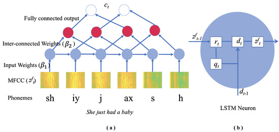
Figure 4. (a) Topology of LSTM for speech classification. The audio signal input is split into a sequence of phonemes. (b) Each LSTM neuron has an input ($r_t$) and a forget gate ($q_t$).

We denote the probability of each phoneme at time index t and for emotion class c as $p\left(z_t\right|c)={\beta }_1^t$ and the transition probability between two phonemes t and $t-1$ as $p\left(z_t\right|z_{t-1},c)={\beta }_2^{t,t-1}$. The emotion label $c=\left\{\mathrm{happy},\mathrm{neutral},\mathrm{angry}\right\}$ for a test audio sample is the highest probability class c as follows:

$$\begin{array}{c}\hfill c={max}_c{\sum }_{t=1}^{\mathrm{n}}{\beta }_1^t{\beta }_2^{t,t-1}\end{array}$$

(4)

where $\mathrm{n}$ is the total number of phonemes. Instead of the class probabilities here, we compute and input the weight matrix ${\beta }_1^t$ of dimension $\mathrm{n}\times \mathrm{h}$ that determines the significance of phoneme $z_t$ for emotion class c modeled by $\mathrm{h}$ hidden neurons. Similarly, instead of the transition probabilities here, we compute an inter-connection weight matrix ${\beta }_2^{t,t-1}$ that corresponds to the strength of association between phonemes $z_t$ and $z_{t-1}$.

Now, the rate of change in the audio signal or gradients over time is given by:

$$\begin{array}{ccc}\hfill \frac{dx\left(t\right)}{dt}& =& {\beta }_1^{t}x(t-\mathrm{h})+{\beta }_2^{t,t-1}s\left(x\left(t\right)\right)\hfill \end{array}$$

(5)

where $\mathrm{h}$ is the maximum time delay and $s\left(x\right(t\left)\right)$ is the oral cavity transfer function defined in Equation (3). The value and direction of gradients can predict which word is going to be formed by the sequence of phonemes. Here, we can also use the memory of past phoneme labels. As shown in Figure 5a, the RNN uses duplicate hidden neurons to model each additional time delay. With increasing delay, the gradients in Equation (5) keep on getting smaller and the model stops updating the weights. The LSTM model that uses a cascade architecture shown in Figure 5b is able to overcome this problem.

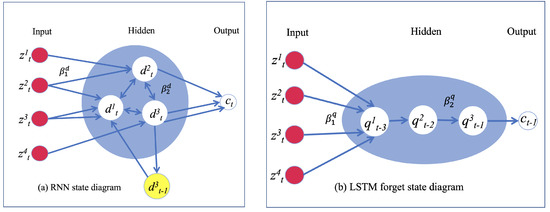
Figure 5. (a) RNN uses duplicate hidden neurons to model each additional time delay. (b) The LSTM model instead uses a cascade architecture to remember the past.

3.3. Audio Spectogram

The raw audio signal has a lot of noise; hence, we represent each phoneme as a vector of features. The human ear is unable to judge differences in high-pitch sounds, also known as high frequencies. The Mel scale has been designed to detect 39 features commonly perceived by human ears. We can use the following equation to calibrate any observed sound to the Mel scale:

$$\begin{array}{c}\hfill f_{mel}=1127.log\left(1+\frac{f}{700}\right)\end{array}$$

(6)

where f is the observed frequency and $f_{mel}$ is the calibrated frequency using the Mel scale.

In order to convert the shape of the oral cavity into sounds and understand its characteristics, we use the Fourier transform. A Fourier transform computes the energy of each frequency or impulse in a sound signal and converts each phoneme from time domain $z_t$ into the frequency domain $z_t^f$. Frequencies with high repetition will result in a peak in the Fourier transform. Following previous authors, we use a window size of $0.03\ast f_s$ to split the audio into impulses or phonemes where $f_s$ is the sampling frequency of the audio. Next, we can phase shift the impulse output over time and take the summation as follows:

$$\begin{array}{c}\hfill z_t^f=\frac{1}{\mathrm{l}}{\sum }_{t=0}^{\mathrm{l}-1}{z}_t{e}^{i2\pi f\frac{t}{T}}\forall f\end{array}$$

(7)

where f ranges over all frequencies in a desired range. As such, a single audio signal is broken down into individual frequencies. We can then look for cycles or patterns at each frequency. This spectrum is then matched with known human filters in the Mel scale filter bank. For example, the microphone noise will not match any filter and can be discarded. The shape of the vocal tract made of tongue and teeth determines how sounds are generated by each individual. As a result, there is a large variance in the pronunciation of words among individuals. Here, each phoneme is converted to a vector of 39 floating points that represent the intensity of each Mel feature in that particular phoneme. These features are referred to as Mel-frequency cepstral coefficients (MFCCs).

4. Speech Emotion Recognition

In this section, we first describe the conventional speech emotion recognition using the Bi-LSTM model. Then, we explain the Affectivespace of concepts where each dimension corresponds to an emotion and a new metric for matching signals. Lastly, we propose a new metric to select the best augmentations for a given training audio.

4.1. Bidirectional Long Short-Term Memory

The LSTM shown in Figure 5b uses a cascade architecture to remember past phonemes in a sequence. The input from the previous hidden neuron $z_{t-1}^f$ in a sequence of phonemes is used to learn the weights of the next phoneme. The predicted label at each time point, $c_t$ is a summation over past $\mathrm{h}$ phonemes. As such, it is able to remember the past without any additional neurons. This reduces the problem of vanishing gradients.

Another solution is to only update the weights for useful phonemes and ignore words such as ‘a’, ‘an’, etc. that are not relevant to the sentiment of the audio. This is achieved in Figure 4b where the model learns the weights of four different states simultaneously, namely: the input gate $r_t$, the forget gate $q_t$, the cell hidden state $d_{t-1}$ and the predicted label $c_t$. The forget gate uses the sigmoid activation function $\mathrm{sig}\left(\right)$ that transforms the input in the range $[0,1]$ where a value 0 indicates that the information is forgotten, as shown in Figure 5b. Furthermore, the additional gates will prevent the gradients from vanishing to zero.

The model is trained using a gradient descent similar to the one described for recurrent neural networks in Equation (5). The continuous state of each gate is determined as a weighted sum of all input nodes:

$$\begin{array}{ccc}\hfill r_t& =& \mathrm{sig}(z_t^f{\beta }_1^r+z_{t-1}^f{\beta }_2^r)\hfill \\ \hfill q_t& =& \mathrm{sig}(z_t^f{\beta }_1^q+z_{t-1}^f{\beta }_2^q)\hfill \\ \hfill d_t& =& \mathrm{sig}(z_t^f{\beta }_1^d+z_{t-1}^f{\beta }_2^d)\hfill \\ \hfill c_t& =& \tanh (z_t^f{\beta }_1^c+z_{t-1}^f{\beta }_2^c)\hfill \\ \hfill {\widehat{c}}_t& =& q_t\odot {\widehat{c}}_{t-1}+r_t\odot c_t\hfill \end{array}$$

(8)

where ⊙ is the element-wise dot product and the gates are updated using the error computed at the last hidden neuron ${\widehat{c}}_t$ and the known target label c. The $\tanh \left(\right)$ is the hyperbolic tangent function that transforms the output in the range of $[-1,1]$. This prevents the exploding of weights because of repeating occurrences of the same words in the dataset. The bi-directional LSTM (BiLSTM) has two LSTMs that are simultaneously trained in opposite directions. One of them remembers the past and the other remembers the future. The weights of the two LSTMs are shared to predict the output sentiment label. As preprocessing, we use GMM to extract the principal components from the MFCC vectors for each phoneme.

4.2. Affectivespace

SenticNet is a network where nodes are concepts and edges determine the relationship, such as ‘IsA’ or ‘HasA’ [33]. We performed a dimensionality reduction on SenticNet from 200K to 100 using SVD. Semantically related concepts will lie close together in the new Affectivespace. The Hourglass model [34] of emotions classifies Level-1 emotions such as ‘Pleasantness’ and ‘Sensitivity’ and Level-2 emotions, which are formed by the composition of these two, such as ‘Joy’ or ‘Anger’.

Figure 6 shows that positive ‘Pleasantness’ results in ‘Joy’ and negative corresponds to ‘Anger’. We can see that concepts in the ‘Anger’ emotion commonly start with the prefix ‘con’ as in ‘confused’ or ‘confine’. Similarly, the concepts in ‘Fear’ emotion commonly start with the prefix ‘ab’ as in ‘abduct’ or ‘abandon’. We can hence conclude that the pronunciation of words can be used to determine the emotional content.

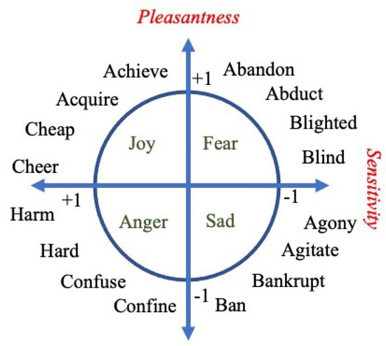
Figure 6. The emotional content in words is often determined by the prefix such as ‘ab’ or ‘con’.

We converted concepts in Affectivespace for three emotions, namely ‘Anger’, ‘Joy’ and ‘Neutral’, into speech. For this, we used text reader software and saved each recording to audio format. To determine the neutral concepts, we constrain the value of both Level 1 emotions to be near zero. Next, we trained an LSTM classifier defined in the previous section to classify the three emotions in concepts. Figure 7 shows that the average accuracy of the model is 62%. It is easier to recognize negative concepts with an accuracy of 70% compared to positive concepts that only have a prediction accuracy of 42%. In this paper, we use a classifier trained on Affectivespace to initialize the LSTM model prior to training on a real-world dataset. This allows us to combine the semantic knowledge of words in addition to the tone of voice.

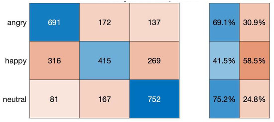
Figure 7. Confusion matrix and accuracy of predicting emotions in audios from Affectivespace.

4.3. Augmentation of Audio

We can increase the number of training audio samples by making slight changes to pitch, amplitude, etc. for known samples and consider $\mathrm{n}$ latent LSTM features in the sample that are learned from the data. We can use a Lyapunov function to ensure stability of Equation (5) and use semi-definite programming to solve it. Here, ⪯ and ⪰ denote the negative semi-definite and positive semi-definite operators. This assumption makes the system convex and has a unique solution. Here, we select the following candidate function $v\left(x\right(t\left)\right)$:

$$\begin{array}{c}\hfill v\left(x\left(t\right)\right)=x^{\mathrm{T}}\mathrm{P}x\left(t\right)+{\int }_{t-\mathrm{h}}^t{s}^{\mathrm{T}}\left(x\left(t\right)\right){\mathrm{O}}^{-2}s\left(x\left(t\right)\right)dt\end{array}$$

(9)

where $\mathrm{P}⪰0$ and $\mathrm{O}⪰0$ are matrices of size $\mathrm{n}\times \mathrm{n}$. For stability, we have to show that the time derivative of $v\left(x\right(t\left)\right)$ is less than 0.

Using Equation (5), the time derivative of $v\left(x\right(t\left)\right)$ can be given by:

$$\begin{array}{ccc}\hfill \frac{v\left(x\right(t\left)\right)}{dt}& =& 2x^{\mathrm{T}}\left(t\right)\mathrm{P}[{\beta }_1^{t}x(t-\mathrm{h})+{\beta }_2^{t,t-1}s\left(x\left(t\right)\right)]\hfill \\ \hfill & +& s^{\mathrm{T}}\left(x\left(t\right)\right){\mathrm{O}}^{-2}s\left(x\left(t\right)\right)-s^{\mathrm{T}}\left(x(t-\mathrm{h})\right){\mathrm{O}}^{-2}s\left(x(t-\mathrm{h})\right)\hfill \end{array}$$

(10)

We can show that, for stability, we require [35]:

$$\begin{array}{ccc}\hfill \frac{v\left(x\right(t\left)\right)}{dt}& =& x^{\mathrm{T}}\left(t\right)\mathrm{H}x\left(t\right)\mathrm{where}\mathrm{H}⪯0\hfill \\ \hfill \mathrm{H}& =& -(\mathrm{P}{\beta }_1^t+{\beta }_1^t\mathrm{P})+\mathrm{P}{\beta }_2^{t,t-1}{\mathrm{O}}^2{{\beta }_2^{t,t-1}}^{\mathrm{T}}\mathrm{P}+{\Sigma }^T{\mathrm{O}}^{-2}\Sigma \hfill \end{array}$$

(11)

where $\Sigma$ is the covariance matrix for $\mathrm{h}$ time delays. We can solve Equation (10) to determine the optimal value of $\mathrm{O}$ for each audio. Table 1 provides the nomenclature of the symbols used in this paper.

Table 1. Nomenclature.

# Symbol	Definition
$v\left(\right)$	Candidate Lyapunov function
$x\left(t\right)$	Sound signal at time point t
$\mathrm{P}$	Unknown positive semi-definite matrix
$\mathrm{O}$	Unknown positive semi-definite matrix
$\mathrm{n}$	Number of phonemes or states in the audio
$\mathrm{h}$	Maximum time delay
$s\left(\right)$	Oral cavity transfer function
${\beta }_1^t$	Input weight matrix of LSTM
${\beta }_2^{t,t-1}$	Interconnection weight matrix between LSTM neurons
$\mathrm{H}$	Unknown positive semi-definite matrix
$\Sigma$	Covariance matrix for sound signal

Lastly, we define the SAM metric as the error between the ${\mathrm{O}}_g$ for the original audio signal $x\left(t\right)$ and the augmented audio signal:

$$\begin{array}{c}\hfill \gamma =MSE({\mathrm{O}}_g,\mathrm{O})\end{array}$$

(12)

where $\gamma$ is the mean-square error (MSE). Since $\mathrm{O}$ is an augmented version of the original ${\mathrm{O}}_g$ signal, we do not think that the normalization of data is needed. We have selected the top 10 augmentations for each audio as we want to reduce the training time without loss in accuracy.

Figure 2 illustrates the flowchart of the proposed audio classification framework. We first trained an LSTM model with concepts from Affectivespace for each of the emotion classes in the dataset. For this, the concepts are converted into audio and the weights of the model are used to initialize the model for a real-world dataset. Next, we enlarge the given training set using various acoustic augmentations such as change in pitch or amplitude. We discard poor quality augmentations with high noise using the proposed SAM metric. The remaining audio signals along with the emotional concepts are used to train a Bi-LSTM speech classifier.

Algorithm 1 explains the complete framework to predict emotions from speech. There are three stages, namely: (I) Enlarging the dataset using augmentation; (II) Preprocessing of the audio dataset; and (III) Training of the audio classifier. In the first stage, we create augmentations from each audio by changing the pitch, amplitude, etc. Next, transform the audio using the oral cavity transfer function defined in Equation (3). To select the best augmentations for training, we match each augmentation with the original audio using Equation (12). We can define an upper threshold of g to select augmentations with low error. In the second stage, we split each good augmentation into individual sounds or phonemes. Next, we convert the phonemes to known MFCC features for humans. The audio signal for each phoneme is now represented as a vector of intensities for 39 MFCC features. The number of phonemes can be very large for some audio recordings; hence, we use GMM to extract a subset of states for the signal. Finally, in the third stage, we used the GMM states for each audio to train a Bi-LSTM classifier for emotions. Instead of starting with random weights for the LSTM during training, we initialized it using weights from a pretrained LSTM for different emotions. To create a pretraining dataset, we selected top concepts for each emotion in Affectivespace and the converted them into sound using a text-to-speech algorithm. Each hidden neuron will learn a word with high frequency in the training data. For example, negative words such as ‘Hard’ or ‘Harm’ with similar sounds will show higher activation for a particular neuron.

Algorithm 1 Framework to Predict Emotions from Speech

1: %Augmentation of Audio 2: forEach Audiodo 3:     Create Augmentations by changing pitch, amplitude, etc. 4:     for Each Augmentation do 5:         Apply Oral Cavity transfer function using Equation (3) 6:         Compute Error $\gamma$ for each audio using Equation (12) 7:         if $\gamma \le g$ then 8:            Add audio to training set 9: %Preprocessing of Audio 10: forEach Training Audiodo 11:     Split each audio into Phonemes 12:     Extract MFCC features for each Phoneme using Equation (7) 13:     Replace each Phoneme with MFCC vector 14:     Extract GMM states for each audio 15: %Train Audio Classifier 16:     Pretrain Bi-LSTM with audios of Affectivespace concepts 17:     Train Bi-LSTM using GMM state features 18:     Test Bi-LSTM on unknown audio

5. Experiments

Validation of the proposed SAM ((available on GitHub github.com/ichaturvedi/semi-definite-audio-matching) Accessed on 2 November 2022) is performed on three real-world datasets: (1) Emotion classification from speech; (2) YouTube product reviews; and (3) Bird identification from audio recordings. Following previous authors, we report the improvement in accuracy over baselines.

Due to the lack of annotated samples, we enlarge our audio dataset using audio-specific augmentation techniques such as pitch shifting, time-scale modification, time shifting, noise addition and volume control. Next, we use the proposed SAM similarity metric to discard augmentations with high noise. Table 2 compares the F-measure of the proposed model with baseline algorithms, namely naive Bayes (NB), GMM, Wav2vec, random forest (RF), k-nearest neighbor (k-NN) and LSTM. The first five baselines are trained on the MFCC extracted from the audio signals, however, they have no memory states.

Table 2. Comparison of F-measure with baselines for emotion prediction.

Dataset	# Classifier	Happy	Angry	Neutral	Total
Emotion	Naive Bayes	0.35	0.49	0.41	0.42
	GMM	0.46	0.49	0.39	0.45
	Wav2vec	0.54	0.5	0.28	0.44
	Random Forest	0.57	0.63	0.38	0.56
	k-NN	0.59	0.6	0.52	0.58
	LSTM	0.52	0.67	0.48	0.56
	SAM	0.76	0.81	0.77	0.78
YouTube	Naive Bayes	0.31	0.63	0.01	0.3
	GMM	0.51	0.42	0.27	0.40
	Wav2vec	0.61	0.27	0	0.29
	Random Forest	0.39	0.6	0.01	0.32
	k-NN	0.41	0.52	0.12	0.34
	LSTM	0.4	0.33	0.15	0.29
	SAM	0.68	0.54	0.1	0.44

5.1. Emotion Classification from Speech

We consider the automatic prediction of the emotional state of a speaker from their speech audio. The RAVDESS dataset contains audio recordings of the same sentence when spoken with different emotions. Furthermore, the same sentence is recorded by both male and female participants. For example, ‘dogs are barking by the door’ can be spoken both with surprise as well as with anger. The dataset has several different emotions, such as calm, happy, neutral, etc., which were collected from 24 males and females. The emotional intensity varies from normal to strong.

We perform 10-fold crossvalidation by training the model on the 9/10th of the speakers and testing it on the remaining speakers. We consider a three-class model of angry, neutral and happy speech audio. As shown in Table 3, we have 192 samples for angry and happy emotions and 96 samples for neutral emotions. Table 4 illustrates an example of the error between the original signal and two augmentations shown in Figure 8. We can see that the MSE for both the clean augmentation and the noisy augmentation is almost the same (0.2). Instead, if we use the proposed SAM metric, the error for the clean signal is much smaller than the noisy signal. Hence, we can easily identify and discard noisy samples that will reduce the accuracy of the trained model.

Table 3. Number of training samples in each dataset.

Dataset	Happy	Angry	Neutral	Total
Emotion	192	192	96	480
YouTube	248	202	48	498
	Bird 1	Bird 2	Bird 3	Total
BirdCall	100	100	98	298

Table 4. Error of Augmented Audio with respect to Ground Truth Audio in the Emotion dataset.

Method	Clean Augmentation	Noisy Augmentation
MSE	0.0151	0.0209
SAM	0.000248	0.5395

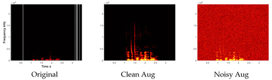
Figure 8. Comparison of the spectrogram of the original audio with a clean and noisy augmentation.

Table 2 compares the proposed method with baseline algorithms for audio classification. We can outperform random forest, k-nearest neighbors (k-NN) and LSTM by over 10% in F-measure. A bigger improvement of 20% is seen over naive Bayes, GMM [36] and Wav2vec [37]. Even for the neutral class with fewer annotated samples, our method shows a 77% F-measure. Wav2vec performs very poorly in a neutral class with only a 30% F-measure. This could be because it uses pretrained vector representation for each phoneme, and hence, it does not generalize well to the current dataset. This dataset is imbalanced as only a few neutral samples are available. The Cohen Kappa statistic measures the robustness of a classifier to such bias in training samples. Figure 9 shows that the proposed SAM has a 0.64 Kappa value, which is significantly higher than baselines such as RF with a Kappa value of 0.3. NB has the lowest Kappa value of 0.15.

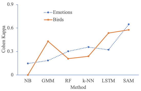
Figure 9. Comparison of Cohen Kappa statistics for different baselines on the Emotion and Bird datasets.

5.2. Spanish Product Reviews Video Dataset

In order to evaluate our model on a cross-language task, we consider MOUD Spanish product reviews available on YouTube [31]. This dataset is searched using keywords such as ‘favorite perfume or movie’ and contains 80 different products. For this paper, we only consider the audio signal of each utterance or phrase that has been manually annotated as positive, negative or neutral. Hence, each video has both positive and negative comments on the product. Following [38], we consider 498 utterances labeled positive, negative or neutral. As shown in Table 3, we have 248 samples for happy, 202 samples for angry and only 48 samples for the neutral emotion. Here again, we perform 10-fold crossvalidation by training the model on 9/10th of the speakers and testing it on the remaining speakers. We consider a three-class model of angry, neutral and happy speech audio.

Table 2 compares the proposed method with baseline algorithms for audio classification. We can outperform naive Bayes, Wav2vec and LSTM by over 15% in F-measure. A smaller improvement of 10% is seen over random forests and k-NN. The improvement over GMM is only 4%. This could be because Affectivespace is in English and hence does not fit well with Spanish sounds. GMM also performs best in neutral class with only 48 training samples. Our method only shows a 10% F-measure for neutral, since the dataset is imbalanced for this class. All the models appear to perform better in happy emotions compared to anger.

5.3. BirdCall Identification

Next, we consider the Cornell Lab BirdCall Identification dataset [32]. It contains audio samples includes 264 different species of birds. These data of individual bird calls have been uploaded by users from all over the world to xenocarto.org. There might be background noise in the recordings, such as other birds and airplane sounds. We consider three species with 100 recordings each, namely: Bird 1 ( Alder Flycatcher), Bird 2 (Canada Warbler) and Bird 3 (Yellow-Throated Vireo). Each recording is approximately one minute long. Due to the complexity of the recordings, the annotations are weak and may contain errors. We perform a 10-fold crossvalidation by training the model on the 9/10th of the recordings and testing it on the remaining recordings. A balanced dataset of all three bird types is used for training. We consider a three-class model of Bird 1, Bird 2, and Bird 3 sound recordings.

Table 5 compares the proposed method with baseline algorithms for audio classification. The biggest improvement is over Naive Bayes, which only shows a 23% F-measure compared to the 72% achieved by our model. An improvement of 10% is seen over GMM and an improvement of 20% is seen over the other algorithms. The proposed SAM works well on all three bird types. The baselines also show similar performance on all bird types except for naive Bayes, which showed only a 16% F-measure on Bird 2. Here again, we computed the Cohen Kappa statistic to measure the robustness of the classifier to bias in the number of training samples for each class. Figure 9 shows that the proposed SAM has a 0.58 Kappa value, which is significantly higher than the baselines such as RF with a Kappa value of 0.2. NB has the lowest Kappa value of 0.01.

Table 5. Comparison of F-measure with baselines for BirdCall identification.

# Classifier	Bird1	Bird2	Bird3	Total
Naive Bayes	0.07	0.16	0.46	0.23
GMM	0.59	0.66	0. 60	0.62
Random Forest	0.49	0.47	0.44	0.47
k-NN	0.49	0.44	0.45	0.46
LSTM	0.46	0.49	0. 45	0.47
SAM	0.67	0.77	0.72	0.72

5.4. Parameters

The number of phonemes can be very large for some utterances. We hence fit the extracted MFCC features to a Gaussian distribution. Now, each state in the time series is a mixture of several Gaussians. To determine the number of states or components in the GMM, we looked at the prediction margin on the baseline Naive Bayes classifier. Here the margin is the difference between the probability predicted for the actual class and the highest probability predicted for the other classes. Figure 10 illustrates the prediction margin versus a principal component of the RAVDESS emotion dataset. Here, samples with the label happy are shown in blue, angry is shown as red and neutral is shown in green. The cross symbol denotes training samples, and the squares are the test samples. A good classifier will increase the margin on the training data and hence have a better performance on the test data. We can see that, among the 20 components, there is poor separation of the three emotions. The separation between the red and blue is more distinct with 10 components compared to 5. Hence, we set the number of components in the GMM to 10 for this dataset. The features fitted to the GMM are then used to train the LSTM model.

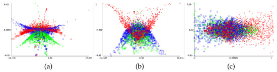
Figure 10. Prediction margin for different number of principal components (a) 5 (b) 10 (c) 20.

6. Conclusions

Presence of neutral comments makes it difficult to understand the emotional state of a person from their voice recording. Only a specific range of frequencies are audible to the human ear. Hence, in this paper, we propose a new audio matching metric that determines the usefulness of a particular sound signal in emotion classification. We leverage the similar pronunciations of negative and positive words in the English language. The classification accuracy of spoken concepts with different emotional content is over 70%. Hence, we conclude that the semantic meaning and tone of voice are both crucial for emotion recognition. Experiments on two real-world emotion datasets show an improvement in the range of 10–20% on the identification of three types of emotions. For the first dataset that includes the lab recordings of different emotional intensities, we see a 20–40% increase in the ‘neutral’ emotion class over baselines. Next, we evaluate our approach on YouTube videos crawled for a particular product. Here, we observed that for each emotion, a different baseline gave the highest accuracy. However, our approach showed the highest overall accuracy in the range of 5–15%. Lastly, to test the generalization of the model to other audio problems, we considered the bird identification from audio recordings and find that we have an improvement in overall accuracy in the range of 10–40%. Future work would be to enhance the audio prediction using phonetic features [39]. This would capture mispronounced words or concepts and normalize them to their standard form.

References

- Cambria, E.; Schuller, B.; Liu, B.; Wang, H.; Havasi, C. Statistical approaches to concept-level sentiment analysis. IEEE Intell. Syst. 2013, 28, 6–9. [Google Scholar] [CrossRef]
- Latif, S.; Cuayáhuitl, H.; Pervez, F.; Shamshad, F.; Ali, H.S.; Cambria, E. A Survey on Deep Reinforcement Learning for Audio-Based Applications. Artif. Intell. Rev. 2022, 1–48. [Google Scholar] [CrossRef]
- Ragusa, E.; Gastaldo, P.; Zunino, R.; Ferrarotti, M.J.; Rocchia, W.; Decherchi, S. Cognitive insights into sentic spaces using principal paths. Cogn. Comput. 2019, 11, 656–675. [Google Scholar] [CrossRef]
- Satapathy, R.; Pardeshi, S.; Cambria, E. Polarity and Subjectivity Detection with Multitask Learning and BERT Embedding. Future Internet. 2022, 14, 191. [Google Scholar]
- Pandelea, V.; Ragusa, E.; Young, T.; Gastaldo, P.; Cambria, E. Toward hardware-aware deep-learning-based dialogue systems. Neural Comput. Appl. 2021, 34, 10397–10408. [Google Scholar] [CrossRef]
- Chaturvedi, I.; Ong, Y.S.; Tsang, I.; Welsch, R.; Cambria, E. Learning word dependencies in text by means of a deep recurrent belief network. Knowl.-Based Syst. 2016, 108, 144–154. [Google Scholar] [CrossRef]
- Burkhardt, F.; Paeschke, A.; Rolfes, M.; Sendlmeier, W.F.; Weiss, B. A database of German emotional speech. In Proceedings of the INTERSPEECH 2005, Lisbon, Portugal, 4–8 September 2005; pp. 1517–1520. [Google Scholar]
- Satapathy, R.; Cambria, E.; Nanetti, A.; Hussain, A. A Review of Shorthand Systems: From Brachygraphy to Microtext and Beyond. Cogn. Comput. 2020, 12, 778–792. [Google Scholar] [CrossRef]
- Mohamed, A.r.; Dahl, G.E.; Hinton, G. Acoustic Modeling Using Deep Belief Networks. IEEE Trans. Audio Speech Lang. Process. 2012, 20, 14–22. [Google Scholar] [CrossRef]
- Shen, L.; Satta, G.; Joshi, A. Guided learning for bidirectional sequence classification. In Proceedings of the 45th Annual Meeting of the Association of Computational Linguistics, Prague, Czech Republic, 25–27 June 2007; pp. 760–767. [Google Scholar]
- Jain, A.; Zongker, D. Feature selection: Evaluation, application, and small sample performance. IEEE Trans. Pattern Anal. Mach. Intell. 1997, 19, 153–158. [Google Scholar] [CrossRef]
- Ragusa, E.; Apicella, T.; Gianoglio, C.; Zunino, R.; Gastaldo, P. Design and deployment of an image polarity detector with visual attention. Cogn. Comput. 2022, 14, 261–273. [Google Scholar] [CrossRef]
- Oneto, L.; Bisio, F.; Cambria, E.; Anguita, D. Statistical learning theory and ELM for big social data analysis. IEEE Comput. Intell. Mag. 2016, 11, 45–55. [Google Scholar] [CrossRef]
- Cambria, E.; Fu, J.; Bisio, F.; Poria, S. AffectiveSpace 2: Enabling Affective Intuition for Concept-Level Sentiment Analysis. In Proceedings of the AAAI 2015, Austin, TX, USA, 25–30 January 2015; pp. 508–514. [Google Scholar]
- Dahl, G.E.; Yu, D.; Deng, L.; Acero, A. Context-Dependent Pre-Trained Deep Neural Networks for Large-Vocabulary Speech Recognition. IEEE Trans. Audio Speech, Lang. Process. 2012, 20, 30–42. [Google Scholar] [CrossRef]
- Sundermeyer, M.; Ney, H.; Schlüter, R. From Feedforward to Recurrent LSTM Neural Networks for Language Modeling. IEEE Trans. Audio Speech, Lang. Process. 2015, 23, 517–529. [Google Scholar] [CrossRef]
- Chaturvedi, I.; Chen, Q.; Welsch, R.E.; Thapa, K.; Cambria, E. Gaussian correction for adversarial learning of boundaries. Signal Process. Image Commun. 2022, 109, 116841. [Google Scholar] [CrossRef]
- Chaturvedi, I.; Chen, Q.; Cambria, E.; McConnell, D. Landmark calibration for facial expressions and fish classification. Signal Image Video Process. 2022, 16, 377–384. [Google Scholar] [CrossRef]
- Poria, S.; Chaturvedi, I.; Cambria, E.; Hussain, A. Convolutional MKL Based Multimodal Emotion Recognition and Sentiment Analysis. In Proceedings of the ICDM 2016, Barcelona, Spain, 12–15 December 2016; pp. 439–448. [Google Scholar]
- Sheikh, I.A.; Chakraborty, R.; Kopparapu, S.K. Audio-Visual Fusion for Sentiment Classification using Cross-Modal Autoencoder. In Proceedings of the NIPS Vigil Workshop, Montreal, QC, Canada, 3–8 December 2018. [Google Scholar]
- Chaturvedi, I.; Satapathy, R.; Cavallari, S.; Cambria, E. Fuzzy commonsense reasoning for multimodal sentiment analysis. Pattern Recognit. Lett. 2019, 125, 264–270. [Google Scholar] [CrossRef]
- Padilla, J.J.; Kavak, H.; Lynch, C.J.; Gore, R.J.; Diallo, S.Y. Temporal and spatiotemporal investigation of tourist attraction visit sentiment on Twitter. PLoS ONE 2018, 13, e0198857. [Google Scholar] [CrossRef]
- Abbar, S.; Mejova, Y.; Weber, I. You Tweet What You Eat: Studying Food Consumption Through Twitter. In Proceedings of the CHI 2015, Seoul, Korea, 18–23 April 2015; pp. 3197–3206. [Google Scholar]
- Avila, A.R.; O’Shaughnessy, D.; Falk, T.H. Automatic Speaker Verification from Affective Speech Using Gaussian Mixture Model Based Estimation of Neutral Speech Characteristics. Speech Commun. 2021, 132, 21–31. [Google Scholar] [CrossRef]
- Gemmeke, F.J.; Ellis, P.W.D.; Freedman, D.; Jansen, A.; Lawrence, W.; Moore, C.R.; Plakal, M.; Ritter, M. Audio Set: An ontology and human-labeled dataset for audio events. In Proceedings of the ICASSP 2017, New Orleans, LA, USA, 5–9 March 2017; pp. 776–780. [Google Scholar]
- Jalal, M.A.; Loweimi, E.; Moore, R.K.; Hain, T. Learning Temporal Clusters Using Capsule Routing for Speech Emotion Recognition. In Proceedings of the Interspeech 2019, Graz, Austria, 15–19 September 2019; pp. 1701–1705. [Google Scholar]
- Hu, D.; Qian, R.; Jiang, M.; Tan, X.; Wen, S.; Ding, E.; Lin, W.; Dou, D. Discriminative Sounding Objects Localization via Self-supervised Audiovisual Matching. In Proceedings of the Advances in Neural Information Processing Systems 33 (NeurIPS 2020), Virtual, 6–12 December 2020. [Google Scholar]
- Xu, R.; Wu, R.; Ishiwaka, Y.; Vondrick, C.; Zheng, C. Listening to Sounds of Silence for Speech Denoising. Adv. Neural Inf. Process. Syst. 2020, 33, 9633–9648. [Google Scholar]
- Asiri, Y.; Halawani, H.T.; Alghamdi, H.M.; Abdalaha Hamza, S.H.; Abdel-Khalek, S.; Mansour, R.F. Enhanced Seagull Optimization with Natural Language Processing Based Hate Speech Detection and Classification. Appl. Sci. 2022, 12, 8000. [Google Scholar] [CrossRef]
- Livingstone, S.R.; Russo, F.A. The Ryerson Audio-Visual Database of Emotional Speech and Song (RAVDESS): A dynamic, multimodal set of facial and vocal expressions in North American English. PLoS ONE 2018, 13, e0196391. [Google Scholar] [CrossRef] [PubMed]
- Morency, L.P.; Mihalcea, R.; Doshi, P. Towards multimodal sentiment analysis: Harvesting opinions from the web. In Proceedings of the ICMI 2011, Alicante, Spain, 14–18 November 2011; pp. 169–176. [Google Scholar]
- Kahl, S.; Wood, C.M.; Eibl, M.; Klinck, H. BirdNET: A deep learning solution for avian diversity monitoring. Ecol. Informatics 2021, 61, 101236. [Google Scholar] [CrossRef]
- Cambria, E.; Liu, Q.; Decherchi, S.; Xing, F.; Kwok, K. SenticNet 7: A Commonsense-based Neurosymbolic AI Framework for Explainable Sentiment Analysis. In Proceedings of the LREC 2022, Marseille, France, 20–25 June 2022; pp. 3829–3839. [Google Scholar]
- Susanto, Y.; Livingstone, A.; Ng, B.C.; Cambria, E. The Hourglass Model Revisited. IEEE Intell. Syst. 2020, 35, 96–102. [Google Scholar] [CrossRef]
- Arik, S. Stability analysis of delayed neural networks. IEEE Trans. Circuits Syst. Fundam. Theory Appl. 2000, 47, 1089–1092. [Google Scholar] [CrossRef]
- Reynolds, D.; Rose, R. Robust text-independent speaker identification using Gaussian mixture speaker models. IEEE Trans. Speech Audio Process. 1995, 3, 72–83. [Google Scholar] [CrossRef]
- Yi, C.; Zhou, S.; Xu, B. Efficiently Fusing Pretrained Acoustic and Linguistic Encoders for Low-Resource Speech Recognition. IEEE Signal Process. Lett. 2021, 28, 788–792. [Google Scholar] [CrossRef]
- Pérez-Rosas, V.; Mihalcea, R.; Morency, L.P. Utterance-Level Multimodal Sentiment Analysis. In Proceedings of the ACL 2013, Sofia, Bulgaria, 4–9 August 2013; pp. 973–982. [Google Scholar]
- Satapathy, R.; Singh, A.; Cambria, E. Phonsenticnet: A cognitive approach to microtext normalization for concept-level sentiment analysis. In Proceedings of the International Conference on Computational Data and Social Networks 2019, Ho Chi Minh City, Vietnam, 18–20 November 2019; pp. 177–188. [Google Scholar]
Publisher’s Note: MDPI stays neutral with regard to jurisdictional claims in published maps and institutional affiliations. |
© 2022 by the authors. Licensee MDPI, Basel, Switzerland. This article is an open access article distributed under the terms and conditions of the Creative Commons Attribution (CC BY) license (https://creativecommons.org/licenses/by/4.0/).