Abstract
Network simulators are used for the research and development of several types of networks. However, one of the limitations of these simulators is the usage of simplified theoretical models of the Packet Error Rate (PER) at the Physical Layer (PHY) of the IEEE 802.11 family of wireless standards. Although the simplified PHY model can significantly reduce the simulation time, the resulting PER can differ considerably from other more realistic results. In this work, we first study several PER theoretical models. Then, we propose a curve fitting algorithm, which is able to obtain a fast and accurate approximation of other PER models. The curve fitting algorithm uses simulated data as input and outputs the coefficients of a simple model that offers a very accurate approximation of the original PER. Finally, we implemented this approximation in the ns-3 network simulator, thus obtaining high realism since now we can select several theoretical PER models or even a more realistic scenario with the effect of the high Peak-to-Average Power Ratio (PAPR) in the signal. The ns-3 results show how the selection of the PER model at the PHY can significantly impact the Packet Loss Rate (PLR) of a scenario composed of a linear chain of several nodes, one of the simplest multi-hop scenarios.
1. Introduction
The development of Wireless Local Area Network (WLAN) standards has made possible the user’s communications with fixed, portable and moving stations. Nowadays, most of the user’s devices use one or more WLAN standards, such as IEEE 802.11a/g/n/ac/ax. These standards have increased the data rates from 54 Mbps of the 802.11a/g to Gpbs rates with the 802.11ax [1]. Based on these standards, an amendment known as IEEE 802.11p was developed for application on Vehicular Ad-Hoc Networks (VANETs). These networks enable vehicle-to-vehicle and vehicle-to-infrastructure communications [2]. These communications allow different applications of Intelligent Transportation Systems (ITS) such as adaptive cruise control, precise maneuvering, and pedestrian detection [3].
The two main technologies for enabling vehicular communications are the IEEE 802.11p [4] standard and Vehicle-to-everything (V2X) cellular communications [5,6]. Based on the physical layer (PHY) of IEEE 802.11a, IEEE 802.11p uses orthogonal frequency division multiplexing (OFDM) but using a 10 MHz channel. In addition, it is considered that IEEE 802.11p is leading other technologies because it is already deployed in commercial vehicles and presents a number of commercially available products based on it [7]. To fulfill today’s more demanding requirements of vehicular communications, the IEEE 802.11bd is in the last stages of the standardization process. Compared to the 802.11p, the 802.11bd aims to double the range, improve the target speed, offer higher reliability and provide two times higher throughput.
A simulator is a standard tool used for teaching and research evaluation of ad-hoc and vehicular communications [8,9]. The benefits include scalability, reproducibility and rapid prototyping [10]. VANETs simulators can be decomposed into two parts: network simulators focused on protocol design and operation, and mobility generators, which are used to mimic realistic vehicle movements [11]. Therefore, there is an increasing number of works, such as [12,13,14], in the scientific community to improve the realism of VANET simulations.
To achieve fast simulation time, it is common that network simulators use simple theoretical formulas to model the Packet Error Rate (PER) of the physical layer of the 802.11 family of standards. For instance, the open-source ns-3 [10], which is one of the leading network simulators used in VANET research, implements the NIST model [15] as a simple way to calculate the PER. However, there are other theoretical PER models reported in the literature that are not available in most simulators. The suitable model for simulation purposes will depend on the application.
This work focuses on improving the realism of the PHY of Network simulators by proposing a technique to obtain a simple model for implementing several theoretical PER models and even simulated PER models into the PHY. Figure 1 presents the operation of our proposal, where we used both MATLAB and ns-3 simulators but with different purposes. We used MATLAB to analyze the effect of high PAPR over the PER of the IEEE 802.11p PHY. This tool allowed us to simulate the physical and link layers, where we implemented the complete 802.11p PHY and added the PAPR effect in MATLAB. From the results obtained, we obtained adjusted and low-cost PER models that can be integrated into more realistic simulation tools such as ns-3. Unlike MATLAB, ns-3 allows to simulate the whole TCP/IP protocol stack with a high level of realism in almost all its layers and also allows to simulate a large number of network devices. However, at the physical level, it lacks many features to improve its realism since the default version of ns-3 uses a simplified model.
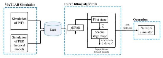
Figure 1.
Operation mode of the proposal.
More precisely, the main contributions of this work are summarized by:
- First, we present a brief survey of the main PER theoretical models found in the literature for AWGN channels and that work with the modulations used in IEEE 802.11p (BPSK, QPSK, 16QAM, 64QAM). Then, using MATLAB, we compare the theoretical models to a complete implementation of the IEEE 802.11p PHY named PhySim-11p [16].
- Second, we analyze the effect of the high Peak to Average Power Ratio (PAPR) problem, which is a main disadvantage of the OFDM technique used in the IEEE 802.11p/bd PHY. Using MATLAB simulations, we present the impact over the PER when a non-linear High Power Amplifier (HPA) is used in the IEEE 802.11p transmitter.
- Third, we propose a curve fitting algorithm, which is able to obtain an inexpensive and accurate approximation of other PER models. The curve fitting algorithm uses simulated data as input and outputs the coefficients of a simple model that offers a very accurate approximation of the original PER.
- Lastly, we obtained adjusted models of the surveyed theoretical PER models and simulation results with the non-linear HPA. Then, these models are implemented in the ns-3 network simulator to improve their realism and tested in a simple scenario to study the effect of the different PER models over the Packet Loss Rate (PLR).
In a nutshell, this paper provides an inexpensive implementation of PER models in ns-3 thanks to a proper fitting procedure. This work laid on PhySim [16], a PHY simulation in MATLAB that aims to facilitate the study of different physical layer phenoms, and extends the results presented in [17], by implementing fitted formulas in ns-3 of a whole set of PER models, including a highly realistic model with PAPR conditions, not available before, all this without extending simulation times.
The rest of this paper is organized as follows: Section 2 presents the related work. Next, Section 3 summarizes the main PER theoretical models found in the literature and compares them with a MATLAB simulation. Then, Section 4 discusses the problems associated with the usage of a non-linear amplifier in the transmitter and presents MATLAB simulation results of its effect over the PHY of IEEE 802.11p. In Section 5, the curve fitting algorithm is presented. Then, Section 6 presents the results of the ns-3 implementation of the fitted models. Finally, Section 7 presents the conclusions obtained from this work.
2. Related Work
The research community has made several efforts to produce reliable network simulations, maintaining the computational cost to be as low as possible. In this regard, the two goals of network simulators are to provide realism and efficiency, where physical layer simulation has a significant role in realism. When it comes to 802.11 PHY layer modeling, the authors of [18] presented Yet Another network simulator (YANS), using Tracing APIs to speed up internal processes. This is achieved by calculating the packet error probability as a function of the cumulative Signal to Interference-Plus-Noise Ratio (SINR), the BER equation, an Additive White Gaussian Noise (AWGN) channel and a hard-decoding Viterbi approach using the first event error probability. In another work, the authors of [15] proposed the NIST model, relying on the same information as the YANS model, except for the difference between the equations of the BER, which uses a Chernoff upper bound. The SINR of the NIST model does not consider the ratio of used-to-total subcarriers in the SINR calculation. Taking into consideration the optimistic Yans model and the pessimistic NIST model, a more realistic model was proposed by the authors of [19], comparing the two models by tuning (i) the SINR equation to consider pilots and cyclic prefix, and (ii) the Viterbi decoder performance by considering the number of erroneous nonzero information bits when an incorrect path is selected. This proposal was shown to more accurately match the MATLAB simulation results of the 802.11a PHY layer.
The IEEE 802.11p VANET communications are being evaluated by several research groups using network simulations. As mentioned above, network simulators must provide high accuracy and realism at the physical layer. In this sense, the reviewed works are focused on analyzing the problems presented by the network simulators to represent the PER, the propagation loss models, error modeling schemes, and the channel models. On the one hand, the authors of [20] highlighted that physical layer variation (in time and/or frequency) should be considered for designing protocols at higher layers. Although this can lead to a higher computing cost for some PHY models, the model is more accurate and more similar to realistic networks. They demonstrated how different the results of the ns-3 simulation are with constant PER compared with a simulator that uses a PER variable. In another work, the authors of [21] presented a comprehensive review of IEEE 802.11 OFDM WLAN PHY WLAN to analyze the problems of ns-3 in the PER and reception process. Then, a multistage reception process is proposed to enhance the realism of the simulation.
On the other hand, a set of propagation loss models is provided by the ns-3 network simulator, which can be used to deploy realistic VANET scenarios. In [13], typical values for propagation and fading loss models are provided to normalize VANET simulations allowing investigators a comparison of their research work. A different paper by the authors of [22] studies the Vehicle-to-Infrastructure (V2I) and Vehicle-to-Vehicle (V2V) scenarios employing real equipment, comparing the results with those obtained in the ns-3 simulator. The conclusion is that simulation models of ns-3 have yet to mature. In [23], the authors incorporated V2V communication into the Ohio State University Vehicle and Traffic simulator (VaTSim) with the ns-3 simulator. The authors state that V2V and V2I urban scenarios present many challenges. Therefore, a propagation model for the urban environment is presented, and the model is validated with experimental data from a test track.
In [24], a survey of different error modeling schemes for wireless communications over fading channels, taking a look at PHY layer error modeling via bit error rate (BER), is presented. Nevertheless, they do not address PER as a useful error modeling parameter nor give mathematical models for it. In another work, the authors of [25] assessed the PHY performance of a VANET by evaluating BER, packet latency, and throughput at different speeds. However, they do not consider the PER in the PHY. In the context of Rate Adaptation Algorithms, the authors of [26] introduce several Rate Adaptation Algorithms for vehicular networks and test them on a vehicular mobility model in OMNET++ and MATLAB. Note that the study focuses on vehicular networks and only considers the problem of rate adaptation without packet loss.
The implementation of more realistic channel models in ns-3 has been addressed by other studies. For example, the authors of [27] presented two error models with bursty behavior for Indoor WLAN channels. Their paper addressed the implementation of a feature that is lacking in ns-3, which is the bursty nature that is characteristic of real wireless channels. In addition, an implementation of the TGn channel is presented in [28] to improve PHY with fading support and which is also suitable for Multiple Input Multiple Output (MIMO) systems. ns-3 is improved for OFDM-MIMO, but at the expense of a considerable increase in computation time. However, they also propose a statistical model to reduce the computation time. In addition, the work of [29] presented the implementation of a spatial channel model for the 0.5–100 GHz spectrum. This work intends to improve PHY by modeling MIMO and other frequency bands for next-generation wireless networks.
There are several papers concerning PER analysis, but it is important to note that first, we focused on PER models for AWGN channels and second, we selected PER models that work with the modulations used in IEEE 802.11p (BPSK, QPSK, 16QAM, 64QAM). For instance, the works in [30,31,32] are focused on BPSK modulation and thus are limited to only two of the IEEE 802.11 data rates. The work in [33] only presents the uncoded PER; therefore, it cannot be applied to IEEE 802.11p, which uses convolutional coding. Additionally, the works in [30,31,32,33,34] are focused on fading channel, while our focus is on the AWGN channel. Finally, the work in [35] is a very small survey of the PER models and is focused on fading channels.
This work is based on the work presented in [17], but this current manuscript includes important contributions that differ in several aspects: (i) we include a brief survey of the main theoretical PER models; (ii) we have combined more PER models with different BER models if feasible; (iii) we have performed a deeper analysis of the results, where we have analyzed the complexity of the models and also evaluated their performance in terms of packet losses. In particular, we have evaluated the leading PER models in MATLAB, demonstrating that our fitted models have a low computational cost. Next, we implemented these models in the ns-3 network simulator to improve the realism of the physical layer.
3. Theoretical PER Models
A search for PER theoretical models that could be applied to vehicular environments in AWGN channels for BPSK, QPSK, 16QAM, 64QAM and convolutional coding was performed. We looked for these models so we could compare them to simulations of the complete IEEE 802.11p PHY. Many of the following PER models are computed from a BER value, which may or may not be given in the corresponding literature in a closed form; therefore, where the BER is a parameter, we use various BER theoretical models to provide different results.
3.1. Fundamentals
The BER is a measure of the received bits that are different from the corresponding transmitted bits (i.e., failed bits) regarding the total amount of bits sent. It is the mathematical, adimensional ratio that can be expressed in decibels. It is defined as:
where is the number of failed bits and is the total number of transmitted bits. A bit is considered erroneous if its value at reception is different from its value at transmission.
The PER is an analogous parameter to the BER in that it is a measure of the amount of failed packets (controlled arrangement of bits) that arrive at the receptor. It is defined as:
where is the number of failed packets at reception, and is the total number of transmitted packets. A packet is considered failed if at least one bit in it is erroneous.
The Signal-to-Noise Ratio (SNR) is the ratio between the signal power and the noise power. The parameter is the energy of the bit over the spectral noise density, and its relation to the SNR is given as [36]:
where is the transmission bandwidth, and is the transmission speed.
In the following sections, we will use the following common terminology:
- for the BER.
- for the SNR.
- L for the packet length in bits.
- for the Q function [37,38].
Additional notation will be explained where presented.
3.2. Classic PER Model
Taking into consideration that a packet is an arrangement of bits, we find the classical relation between PER and BER as [39]:
This expression considers that the probability of successful reception of each bit is independent of the rest in the packet and equal to . Its derivation comes from this fact and is fairly straightforward.
3.3. Abrate et al. PER Model
In [40], a simple mathematical parametric model for PER calculation is presented. It depends on the SNR and the length of the packet, and it takes eight parameters, which are represented in a table, a row for each transmission speed of the standard. The model is formulated as:
where and are intermediate parameters defined as:
The parameters and () are defined for each of the eight transmission speeds allowed by the standard. An 8 × 8 table is presented in [40] containing the values of these parameters. The constant c is an adjustment parameter the authors introduced to more closely fit the model to the empirical data, which considers transmissions in vehicular networks.
This model is of particular interest, as the formulation lets us use it to perform further curve fitting for other models. Indeed, this model is the one that will be used to fit the other models presented in this work.
3.4. Mahmood and Janti PER Model
In [39], the authors provide, through an Extreme Value Theory (EVT) approach, a PER model that takes into account the structure of the BER definition. In the paper, they specify a standard definition for the BER as follows:
where and depend on the modulation scheme. Then, the PER model is given as:
where and are defined as:
where is the inverse error function, and e is Euler’s number.
This model considers arbitrary modulated transmissions over an Additive White Gaussian Noise (AWGN) channel.
3.5. Song and Choi PER Model
In [36], the authors propose an upper bound for PER in OFDM systems. The PER model is given by the following inequality:
where is the free distance of a convolutional code, is the number of paths in the trellis of length d, and is a parameter defined as:
where is the BER for the modulation scheme .
Notice how the structure of the PER bound is the same as the classic PER model (Equation (4)); however, in this case, we have a different term in place of the term. The sum term is related to the convolutional encoding of the OFDM system. It describes how likely it is to have a bit error for the modulation scheme considering a convolutional code with free distance .
Here it is helpful to consider error rate parameters as probabilities of error occurrences, which is a valid way of looking at them, considering them as predictors for errors. In other words, the sum term describes the likelihood that an error occurs for every code distance d greater than the free distance (the smallest distance in the code between two codewords). This probability is obtained by multiplying the likelihood of an error for a codeword length d by the number of codewords of length d (paths of length d in the trellis ). The likelihood of a bit error for a given value of d is given by .
The parameter adds up the different probabilities of cases where there are at least k errors in an array of d bits (codeword), with k going from half the value of d (half of the bits are erroneous) to the value of d (all of the bits are erroneous). This is achieved by a simple binomial distribution for each value of k with parameter since that is the probability of a single bit being erroneous. Then we add up the binomial distribution outputs for all the values of k considered, which is a measure of the likelihood of having an erroneous codeword of length d.
The authors also take into consideration a bit energy per noise density specific for OFDM systems , which is given by:
where is the bandwidth for the OFDM symbol, is the transmission speed, and M is the number of symbols per modulation scheme. The constant in the expression refers to the portion of the OFDM symbol, not considering the cyclic prefix. Since this model works for OFDM systems, every process involved is implied. The transmission goes over an AWGN channel.
In the ns-3 software, the Yans PER model is the same as the Song and Choi model, taking into account only the first two elements of the PER summation presented in Equation (12). This fact makes the ns-3 Yans model a less precise version of the Song and Choi model, so we will not consider it.
3.6. Khalili and Salamatian PER Model
In [41], the authors propose a PER model that considers residual physical layer errors after decoding the convolutional coded signal, stating that errors in different bits are not independent. The approach treats the convolutional code as a block code by using a code termination technique. Therefore, they analyze the error event distribution considering the convolutional code parameters.
The errors at the output of the convolutional decoding (typically by the Viterbi algorithm) are considered not to be uniform or independent, so the authors analyze the distribution of such errors. To simplify the analysis, they use a code termination technique on the convolutional code to simplify the analysis.
For a convolutional code of constraint length K, the code termination technique consists of cutting the output of the code after bits, where the last K bits are logical zeros (this forces the code to its initial state). Hence, the convolutional code can be seen as a block code of length , where n is the number of simultaneous output bits per k input bits from the convolutional code (the convolutional code rate r is given by ). The rate of the corresponding block code is now:
The Event Error Rate (EER) as a function of the SNR is given by:
where is the free distance of the code and is the number of paths of length in the trellis. Here, it is worth recalling that an error event is the number of bits that present a decoding path in the Trellis that is different from the corresponding coding path, plus K bits without error (i.e., bits that follow the same trellis path in the decoding process as is in the coding process).
The authors assume that the path length in the Trellis of a period without errors follows a geometric distribution of parameter . Therefore, the PER (i.e., the probability of having at least one bit error in a packet of length N) is the CDF of a geometric distribution of parameter for a number N of trials (bits in the packet). Then, the general PER model is given by:
which has the same structure as the classical PER model (Equation (4)); however, to obtain the value for , we go through the following derivation: we define as the mean length of an errorless period, which is given by
where is the length of a decoding epoch, which consists of an errorless period followed by an error event, and is the average error event length. Therefore, on the one hand, we have, because of the way the EER is defined:
and on the other hand, to define , the authors come to the following expression using the block code approximation:
is the inverse of the mean length of an errorless period; therefore, by using Equations (18,19,20), we come to the following expression:
This model only considers arbitrary convolutional coding for a BPSK modulation scheme.
3.7. ns-3 Software NIST PER Model
The ns-3 simulation software provides us with two PER models, which it uses in wifi scenarios: the Yans model and the NIST model. The NIST model, which is the most accurate of the two [15], is given by:
where is the free distance of a convolutional code, d values and the values are convolutional code parameters and b depends on the convolutional code also. The value of n is 17 for and 10 for the other allowed rates, this is because for every other value of is zero.
This model, similar to the one referenced in Section 3.5, tries to account for the errors due to the modulation and convolutional encoding.
Similarly to Equation (12) a sum is introduced in which it accounts for codeword lengths or path lengths in the Trellis d from the free distance onward; however, due to computational limitations, the sum does not go to infinity and instead does to a given value . The same idea holds that the sum will provide us with a measure of the likelihood that we will obtain an erroneous packet, which is computed by summing over that likelihood for each value of d multiplied by the number of paths of length d, in the Trellis.
In this case, the measure of that likelihood for each value of d is given by the expression .
3.8. BER Models
Many of the PER models make use of the BER for their calculations and there are several forms of obtaining the BER in the literature. The authors of [42] proposed a simple geometric approach for M-PSK and M-QAM BER Computation. The proposed approximations obtain similar results compared to Monte Carlo simulations. Therefore, we consider that these approximations would give a similar result to the closed-form formulas we selected and are explained in this subsection. The work in [43] proposes five new closed-forms and a novel lower bound of the Gaussian Q-function. Furthermore, it proposed the ASER for a fading channel, but in our work, we only consider an AWGN channel; therefore, it cannot be used. The work in [44] presents a closed-form average bit error rate calculation for the Nakagami-m fading channel, but it differs from our work in the channel considered. While the work in [44] proposes a BER expression for a Nakagami-m fading channel, our work uses BER expressions aimed at a coded AWGN channel.
We selected the BER equations presented in the following mainly because of two reasons. First, we wanted to compare the theoretical PER models against the NIST model used in ns-3 network simulator; thus, we selected the BER formulas used in the NIST model. Second, we selected BER formulas well known in the literature or from other works (such as Song and Choi [36]) so we could compare the results to other proposed PER models.
In [37], we can find theoretical models for BER derivation. Generally, for our modulation schemes of interest, the BER is provided by:
In [36], Song and Choi present their own models for BER derivation:
These equations consider an OFDM symbol adjusted given by (Equation (14)), but they can be used as general BER models by using the classic .
Finally, in [45,46], we have BER models given by:
which are exact and closed-form expressions of the BER for QAM modulations for an AWGN channel when gray code bit mapping is used.
3.9. MATLAB Simulation of PER Models
We implemented a MATLAB simulation of the PER models presented above combined with different BER models when possible. This was done to compare the theoretical PER models versus the PER of the complete IEEE 802.11p PHY, which was also implemented in MATLAB. A description of the implemented theoretical models is as follows:
For Models 1 to 10, the formulas presented in Section 3 were used to plot the PER vs. SNR figures. The PER using the IEEE 802.11p PHY was obtained by a Monte Carlo simulation (described in [16] using an AWGN channel with a linear response HPA, which is a common assumption in all simulators). Table 1 presents the parameters used for the IEEE 802.11p PHY simulation.

Table 1.
Parameters used in the IEEE 802.11p PHY simulation.
Figure 2 presents the results of the PER vs. SNR for a packet length of bytes and different data rates. The ten PER models are plotted in dashed lines. In contrast, the solid black line, called simulation, represents the PER using the IEEE 802.11p PHY simulation. In this figure, we can observe a similar shape of the PER curves (theoretical and simulation). Although, more strictly, models 7 and 8 are the ones more similar in shape to the simulation curve. These models use the classical PER model with similar BER models.
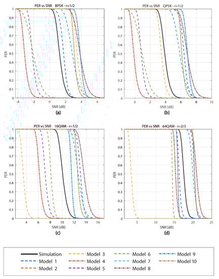
Figure 2.
PER vs. SNR comparison of the models with bytes for (a) 3 Mbps (BPSK R = ), (b) 6 Mbps (QPSK R = ), (c) 12 Mbps (16QAM R = ), (d) 24 Mbps (64QAM R = ).
We can also analyze how close the models are in terms of SNR. Compared with the simulation curve, we can observe that the models have different behaviors depending on the data rate used. Some models are closer to certain data rates but farther in others. The graphs show that model 7 is the closest to the simulation curve having a difference in SNR, which varies from 0 to a maximum of 2.6 dB. Although this difference in SNR is small, analyzing Figure 2c for an dB, model 7 would receive 30% of packets with error against 0% with the simulation curve. Therefore, small differences in SNR can cause a significant change in the PER.
Another interesting result is model 10, which has a difference in SNR varying from 1.5 to 2.5 dB for the different data rates. On the other hand, model 3 keeps getting farther from the simulation curve for higher speeds because model 3 is independent of the modulation scheme. We can also appreciate that models 1, 8, and 10 always behave as upper bounds, while models 4, 5, and 6 always behave as lower bounds. Among models 4, 5, and 6, which use the PER model from Song and Choi (Equation (12)), model 6 is the closer of the three to the simulation curve. Finally, considering models 7, 8, and 9, which use the Classical PER model (Equation (4)), model 7 is the best.
4. PER Simulation with Non-Linear HPA
4.1. Peak-to-Average Power Ratio (PAPR) Problem
Nowadays, OFDM is used in several standards, including the IEEE 802.11 family. The main advantages of OFDM are robustness against multipath fading, high data rate, and high spectral [47] efficiency. Nevertheless, it also has disadvantages such as the high PAPR problem of the time domain signal.
The high PAPR of the OFDM signal occurs when large signal peaks appear. Since the appearance of these peaks depends on the transmitted data, they cannot be predicted. When the high PAPR signals pass through the HPA, it causes interference and distortion due to its non-linear response.
The HPA is in charge of the amplification of the signal, and usually it has a non-linear response to obtain high efficiency. To obtain high efficiency, the non-linear HPA operates near its saturation zone, which is not adequate for a signal with high PAPR. When a large signal peak goes through the non-linear HPA, it surpasses the saturation zone, and thus, it is cut, affecting the signal. Therefore, the non-linear HPA causes non-linear distortions to the OFDM signal with high PAPR. These effects are: increased adjacent channel interference and out-band and in-band distortion.
Several PAPR reduction techniques have been proposed to reduce the effects of the usage of a non-linear HPA with an OFDM signal with high PAPR. Leading techniques include clipping, phase optimization, tone reservation, tone injection, constellation shaping, and selective mapping [48]. These techniques are able to reduce the PAPR but require (depending on the technique) extensive computation, transmission of side information to the receiver, or degradation of the system bit error rate.
4.2. Simulation Results
We also simulated the IEEE 802.11p PHY layer in MATLAB but considered a non-linear HPA. For modeling the HPA, a solid-state power amplifier (SSPA) was considered. The data rates, modulation and coding parameters used for the simulation are shown in Table 2.
Table 2.
Parameters used in the IEEE 802.11p data rates.
We use a non-linear HPA with an Input Back-Off (IBO) of 6 dB at the output of the PHY layer in the MATLAB simulation. Figure 3 presents the PER (in logarithmic scale) vs. the SNR for a packet length of 50 bytes and with linear (solid lines) and non-linear (dashed lines) HPA. The figure shows that for a data rate of 9 Mbps (blue lines), both the linear and non-linear HPA give similar PER. This is because the 9 Mbps data rate uses QPSK modulation, which is more robust against distortions caused by the non-linear HPA. For the 18 Mbps data rate (red lines), a small degradation of about 0.4 dB is caused when the non-linear HPA is used. For 24 Mbps (yellow lines), we can observe a variable degradation, which increases for smaller PER. The degradation is about 1.25 dB for PER = 0.1 and around 5 dB for PER = 0.01. For 27 Mbps (violet lines), we can observe an even bigger degradation. For PER = 0.1, the degradation is around 2.5 dB, while for PER = 0.01 is over 5 dB. Compared to the 9 and 18 Mbps, the 24 and 27 Mbps show a bigger degradation that increases for smaller PER. The reason of this behavior is that 24 and 27 Mbps use 64-QAM modulation, which gives a higher data rate but is less robust against distortions. Therefore, in 24 and 27 Mbps, the distortions caused by the non-linear HPA can not be mitigated by the 64-QAM modulation, causing a big degradation in the PER.
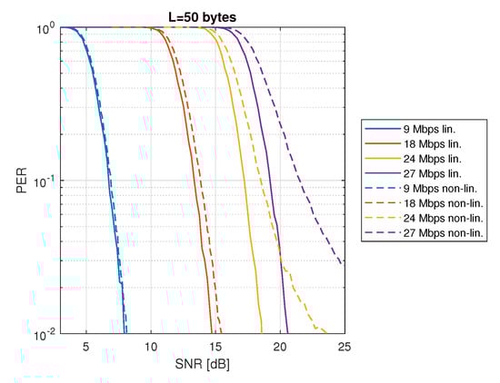
Figure 3.
PER vs. SNR with linear and non–linear HPA (IBO = 6 dB, bytes).
Figure 4 shows the results of using the Orthogonal Pilot Sequence (OPS) technique to reduce the PAPR, taking into account a non-linear HPA with an IBO of 6 dB with a packet length of bytes. The solid lines represent the PER for data rates of 18, 24, and 27 Mbps when the OPS technique is used, whereas the dashed lines show the PER for the same data rates when the PAPR reduction is not used. In the case of 18 Mbps (blue lines), we can observe a small improvement in the PER since in this data rate the effect of the non-linear HPA is also small (see Figure 3). Then, for 24 Mbps (red lines) and 27 Mbps (yellow lines), we can observe an important improvement when the OPS technique is used. In conclusion, the OPS technique, which is used for PAPR reduction, improves the PER, especially for the 24 and 27 Mbps data rates. This is because of the reduction in the signal distortion achieved by the OPS technique. Thus, less signal distortion implies less PER degradation when the less robust 64-QAM modulation is used (24 and 27 Mbps).
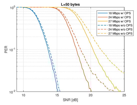
Figure 4.
PER vs. SNR with non–linear HPA (IBO = 6 dB) with and without OPS technique for PAPR reduction ( bytes).
5. Curve Fitting
In previous sections, we presented some theoretical PER models and also simulation results of the PER in the presence of non-linear HPA. To implement these models in the ns-3 simulator, we needed an alternative with low complexity but high accuracy. Additionally, we wanted to use only one model that could implement all other models. Therefore, a curve-fitting process was carried out for the PER curves of the models, which we call the fitted models. The PER data of the fitted models were obtained through simulations and used for the fitting.
From the simulation results of Section 3.9 and the analysis of the theoretical models, we found out that Model 1 (see Section 3.3) can give us high accuracy and low complexity; therefore, it is used for the curve fitting. In this model, there are eight fitting constants (, , , and , , , ) to be determined for each of the eight transmission speeds for each fitted model (we call this a case). That is to say, an 8 × 8 matrix of constants determines a fit. We use two intermediary fitting constants named and for each case in order to obtain the value of the eight constants per case. Since four fitting constants define and , respectively, as a function of the packet length, data for at least four packet lengths per case must be provided.
The fitting process is as follows:
- 1.
- We collect PER data for an SNR range of each case (a transmission speed for a fitted model) on a semi-logarithmic scale for the number of packet lengths chosen. We used eight packet lengths: 75, 250, 750, 1500, 4000, 6000, 9000, and 12,000 bits.
- 2.
- For each case, considering all the packet lengths applied, an automatic first stage fit is made to find the corresponding values for and .
- 3.
- For each case, considering the intermediary fitting constants defined by the packet lengths, a second stage fit is made to find the corresponding values for , , , and , , , .
The first stage fit consists of an automatic fit of the PER models for each of the packet lengths, considering and as the fitting parameters. In our approach, we use as the main adjustment variable and as corrector of the error produced by the fit made using . In this way, the optimization of the two parameters is achieved independently, following a coordinate descent approach. This is, at each iteration of the fitting (case and packet length fixed), we first find the principal component and then the error-corrector component to minimize further the error regarding the PER model. We perform this process by starting from the shortest packet length. As we move up in packet lengths, we enforce that and vary monotonically as a function of the packet length in order to obtain values for and that work well in the second stage fit. The automatic fitting algorithm—applied independently for each packet length of each case- —is shown in Algorithm 1. For a given packet length, we set the initial values and so that the fitting model for PER values corresponds rather well with the data of the PER fitted model within the SNR range. Then, an iterative process is carried out by introducing offsets and to tune parameters and . This is performed separately for each parameter because, as we have anticipated, we use coordinate descent. At each iteration, we update the offset and the initial point to into a Compute_parameter function to obtain a better value and then we do the same for the error component by updating offset and initial point to . Finally, after obtaining the values of and , we check for the differences between these values obtained with the previous iteration , ; if both differences are below the chosen threshold, we have reached convergence for the fitting parameters, and we may stop the process with the current iteration parameters. Otherwise, start the iterative processes once again. Effectively, we are performing an iteration to find convergence for the parameters, and within each of these iterations, we are finding the values of each of the parameters by iterating to find convergence for the CSE using Compute_parameter function (Algorithm 2). We establish a threshold .
| Algorithm 1: Curve Fitting Algorithm |
 |
| Algorithm 2: Compute_parameter |
 |
In a nutshell, Compute_parameter (Algorithm 2) performs the fitting process by updating the parameter at each iteration with the offset and keeping fixed . The algorithm stops in the i-th iteration when the relative difference between CSE and CSE is under the threshold (convergence for CSE).
Regarding the choice of offset values and in Algorithm 1, they have to be small enough to avoid divergence, but not too small as to make convergence slow. In principle, we prefer for them to be small, even if it slows down convergence, as long as it does not diverge. Therefore, at the initial iteration, we have to set a small value of both and considering the usual ranges of and . For the next iterations, the offsets and are set as a multiple of of the difference between the current values of and , and the values of the previous iteration and for avoiding divergence. That is:
We set , , and .
This iterative process is completed automatically for a given packet length L, starting from the lowest length. After the lowest length is done, we move to the next value of packet length. At this point, the tendency of our parameters over the packet lengths becomes relevant.
As stated previously, in order to have reasonable data for our second stage fit, we must ensure that both and are monotonic as the value of L increases (either increasing or decreasing). For this to be fulfilled, after the parameters had been found for two consecutive packet lengths, the algorithms compare those two sets of parameters and determine the tendency, either increasing or decreasing. Then, for the next packet length onward, another condition is introduced in the iteration, which is that the following values of the parameters must follow the tendency, e.g., if is increasing with L, the following value of can not go below the previous one.
The setting up of the initial values for and is completed with the help of a GUI with sliders for the values of and , which includes precision adjustment, parameter monotony check and data saving functionality. The GUI also allows us to automate the data gathering for all the packet lengths of all the cases for all models.
The second stage fit consists of an automatic fitting for the , , , and , , , constants from the and values obtained in the previous stage and the corresponding packet lengths. In this case, we used the MATLAB Curve Fitting Tool. In order to obtain the best fit possible, we iterate this fitting stage multiple times for different, randomized starting points and choose the one with the lowest root mean square error.
We repeat this whole two-stage fitting process for each case of each fitted model to obtain the 8 × 8 parameter matrices of each model. Using the fitting algorithm, we found out that the PER curves for the fitted models resemble the fitting model in sections; therefore, the fit gives a good approximation of a given PER model up to a point in the y-axis. After that point, the fit starts by not approaching the fitted data enough. With this consideration in mind, we take a two-matrix approach. This approach consists of fitting the curves two times: the first one from 0 dB to a threshold in the PER axis, and the second one from to a stopping point . Thus, there are two matrices generated per fit, once for each fitting stage.
The usage of the two-matrix fit is as follows:
- 1.
- Given the SNR value, compute the PER value using the first matrix.
- 2.
- Check if the computed PER value is equal or less than .
- 3.
- If this holds true, compute the PER value once again, this time using the second matrix.
- 4.
- If step two is false, do nothing.
- 5.
- Return the PER value.
We chose the values for and as −10 dB (0.1) and −30 dB (0.001), respectively, considering that these values give a fair fit for the curves.
5.1. Fitting Results
Here, we present the results of a simulation implemented in MATLAB to compare the theoretical models against the curve fitting algorithm presented in Section 5. Based on the analysis presented in Section 3.9, we selected these PER models for the simulation: Mahmood and Janti (model 2), Song and Choi (model 6), Classical PER model (model 7) and ns-3 NIST (model 10). Only these models are used because they are the more precise and for the sake of readability in the following figures.
Figure 5 presents graphs of the PER as a function of SNR for each model as dashed lines (labeled Simulated) and their two-matrix fit in continuous lines (labeled Fitted). Each graph compares the fitted and simulated models for the different modulation and coding rate combinations allowed by the IEEE 802.11p standard. We included only the graphs of Model 2 and Model 6 because of the similar results we obtained for the 10 models. Additionally, we included graphs with linear (a) and logarithmic (b) scales for analyzing the behavior in the low PER region. We can see that the fit approximates the theoretical models very well in both, linear and logarithmic scales. Although, when the PER is higher than 0.8, the curves show a slight difference in the linear scale. The effect of the two-matrix approach is noted in Model 6 (red curve BPSK 1/2) with the linear scale at PER around 0.1; there is a small jump in the PER due to the switch between the two matrices. Something similar can be observed in the logarithmic scale at a PER of around . Regardless of these small differences, for most of the PER range, the fit is very close for all configurations in both scales.
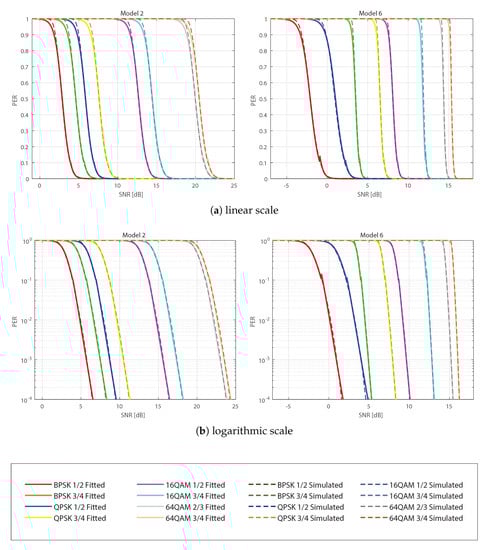
The simulation results show that a very good fit is obtained, and the closeness of the fit is made possible by the 2-matrix approach. These results validate the proposed curve fitting algorithm; therefore, in the next section, we will present the results of the ns-3 implementation of the models.
5.2. Complexity Analysis
A metric to compare the models is the complexity of their implementation. This refers to the maximum number of operations to compute a PER value. It is important to mention that the curve fitting process is performed offline and independently of the final model implementation. Thus, this subsection presents the complexity of the implementation of the two-matrix fit.
For the complexity analysis, we consider a range of operations such as value grabbing, adding, multiplying, exponential, powers and other mathematical functions for the worst case scenario of each model. In particular, integrals and infinite sums are considered to be truncated, where the number of sums performed is unknown and is represented by n. We also consider subtraction to be the addition of negatives, division to be the multiplication of inverses and roots to be the powers of fractional numbers. Hyperbolic tangents, by their exponential definition, can be considered as three multiplications, two exponentials, and two sums. Multiplications and sums are considered basic operations, while exponentials and powers are considered complex operations.
Table 3 summarizes the complexity results of the 10 PER models and the two-matrix fit (called fit). The number of operations shown in the table corresponds to the calculation of the PER for a single SNR value. It is worth noting that the complexity order refers to how the number of operations scales with the number of elements taken to compute the infinite sums or the integrals in each case, not with the SNR range or value.
Table 3.
Complexity analysis results.
An ordered sequence for the models according to their complexity is not apparent by looking at the table, in part because we are comparing functions that may have different implementations, which may lead to different internal complexities, and the number of operations for infinite sums or integrals is not determined. However, we can see that Models 1, 3, and the Fit have the lowest complexity because of having a relatively low number of operations and do not depend on infinite sums or integrals. Therefore, we can affirm that by using the proposed two-matrix fit model, we obtain one of the lowest complexities compared to the other theoretical models.
6. ns-3 Simulation
We implemented the two-matrix fit model in ns-3 to evaluate the ten theoretical PER models and the PER with non-linear HPA over scenarios that use IEEE 802.11p. It is worth noting that since the entire fitting process is performed offline and independently, there is no additional computational cost incurred in the ns-3 simulation. The only requirement is to compute Equation (5) twice for each packet received.
Figure 6 presents the ns-3 simulation scenario, which consists of a linear chain topology of static nodes separated at a certain fixed distance. This separation allows communication only with the next node and the source and sink nodes located at both ends. We have used the Optimized Link State Routing (OLSR) protocol to obtain the address of the next node for communication, although OLSR is unsuitable for VANETs, and furthermore, to obtain the routing table and send messages in our chain scenario, any routing protocol, even just CAM packets. The goal is to assess the PHY layer, not the network layer or the performance of any routing protocol. In addition, the code is available for use by the scientific community in [49].
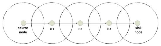
Figure 6.
Linear chain topology of five nodes. Source + 3 relays + sink.
The simulation parameters are summarized in Table 4.
Table 4.
Simulation settings.
6.1. PER of Theoretical Models
Figure 7 presents the Packet Loss Rate (PLR), which is obtained by dividing the number of packets not received by the total number of packets versus the distance for different data rates and theoretical models for a packet size of 50 bytes. For readability, only the results for Models 2, 4, 5, 6, 7, 8, and 9 are included. Figure 7a shows the PLR obtained in the last of a chain of two nodes for 18, 24, and 27 Mbps. For 18 Mbps, we can observe that the PLR varies drastically depending on the model. Considering a PLR of 0.5, the distance between nodes with Model 8 is around 215 m, while for Model 4, it is around 315 m. Thus, for the same scenario of two nodes and 18 Mbps, the distance between nodes for achieving a PLR of 0.5 can differ by around 100 m. When comparing the 18 and 24 Mbps data rates, we can see a similar trend in Models 2, 4, 5, 7, and 8; however, Models 6 and 9 have different results, which are explained due to the different impacts of modulation and coding rate over some models. Furthermore, for 24 Mbps and a PLR of 0.5, we can observe a difference of around 90 m for the most opposite models. Similarly, for 27 Mbps, we observe different results compared to the previous cases and a difference of around 70 m between the most opposite models. Figure 7b shows the PLR obtained in the last of a chain of three nodes for the same data rates explained previously. If we compare this case to the chain of two nodes, we observe a similar trend in the shape and position of the curves. The main difference is that with the chain of three nodes, the curves are shifted to the left; thus, for achieving the same PLR, the distance between nodes is reduced. In the case of Figure 7c, which considers a chain of four nodes, we can see a smaller difference in the distance compared to the three nodes case.
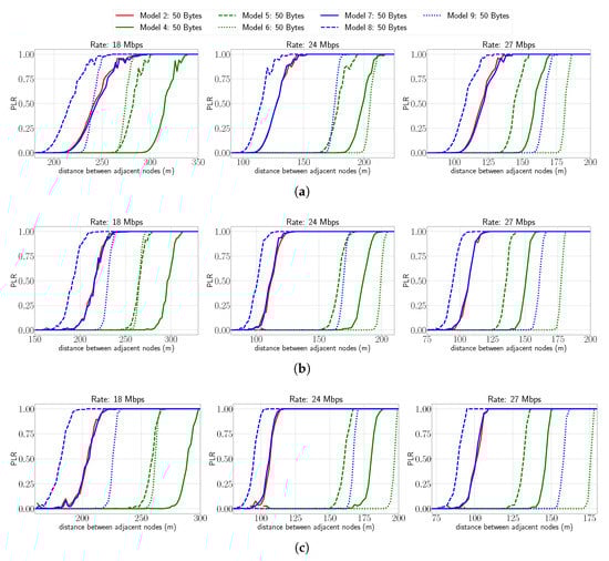
Figure 7.
PLR vs. distance for different rates and for different linear chain topologies. Approximation of theoretical models with packet size of 50 bytes. (a) Number of nodes: 2, (b) number of nodes: 3, (c) number of nodes: 4.
In the same way, Figure 8 presents the PLR versus the distance for different data rates and theoretical models for a packet size of 500 bytes. Compared to Figure 7, we can observe a very similar trend and shape of the curves for the different data rates and number of nodes. The only difference is a small shift of the curves to the left due to the increased packet size, which reduces the distance between nodes for a given PLR.
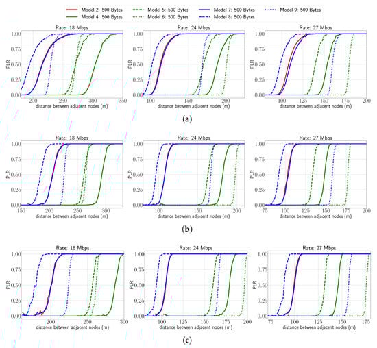
Figure 8.
PLR vs. distance for different rates and for different linear chain topologies. Approximation of theoretical models with packet size of 500 bytes. (a) Number of nodes: 2, (b) number of nodes: 3, (c) number of nodes: 4.
From these results, we can conclude that the impact of selecting different theoretical models of the PHY is not negligible in the PLR. We observed a difference as big as 100 m between the most opposite models for a given PLR.
6.2. PER with Non-Linear HPA
In this subsection, we present results obtained with the fitted models to analyze the impact of the non-linear HPA and to show that it is possible to transfer the behavior of the non-linear HPA into ns-3. In Figure 9, the PLR vs. distance for different models, data rates, and packet sizes is presented. The figure shows the curves of the NIST model in green, which is the default mode in ns-3 for modeling the PHY in the IEEE 802.11p. The results are presented in blue for the linear HPA, in magenta for the non-linear HPA, and red for the non-linear HPA using OPS for PAPR reduction (labeled HPA w/OPS). Additionally, the solid lines are the curves for 50 bytes packet size, while the dashed lines are for the 500 bytes case. Figure 9a depicts the PLR attained at the last of a two-node chain (the first node is the source and the second node is the sink) for 18, 24, and 27 Mbps. In the case of 18 Mbps, we can observe a similar PLR for the linear HPA, non-linear HPA and HPA with OPS. This correlates with the Matlab simulations, where we showed that the effect of the non-linear HPA is very small for this data rate. On the other hand, we can observe a big gap between the NIST model and the others, being the NIST model the one with the worst PLR. The results for 24 Mbps show the effect of the non-linear HPA causing degradation of the PLR. The degradation is small for the 50 bytes case, while for the 500 bytes packet size, the degradation is much more noticeable. Similarly to the 18 Mbps data rate, the NIST model gives the worst PLR. The results for 27 Mbps are similar to those obtained for 24 Mbps. However, a slightly higher difference is noticeable between the curves of the three models. In conclusion, for 24 and 27 Mbps, the PLR is significantly degraded when using a non-linear HPA at the transmitter. Furthermore, the PLR of the NIST model is shown to be very different and more pessimistic in most cases.
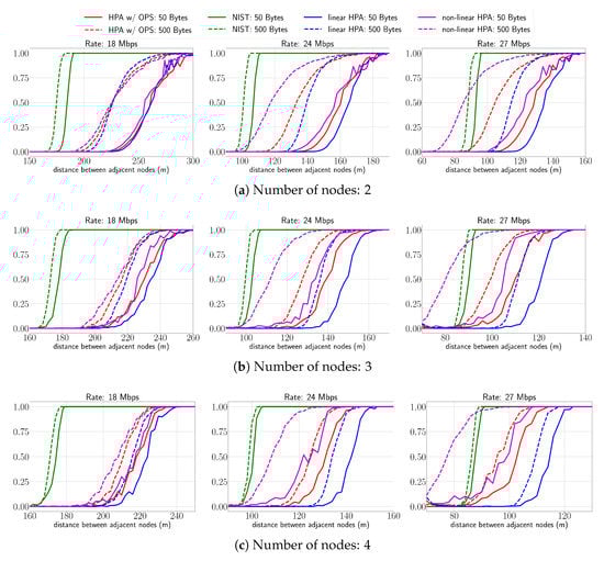
Figure 9.
PLR vs. distance for different rates and for different linear chain topologies. (a) Number of nodes: 2, (b) number of nodes: 3, (c) number of nodes: 4.
Figure 9b shows the PLR obtained at the last of a three-node chain for 18, 24, and 27 Mbps. Similarly to the two-node chain case (a), we can observe that for 18 Mbps the linear HPA, the non-linear HPA, and the HPA with OPS present a small PLR difference for the two packet sizes. For 24 Mbps, we can see a much bigger difference between the three models, the reason for this result being the additional node, which increases the total PLR. For the 27 Mbps, the results are similar to the 24 Mbps but with an increase in the PLR degradation. Finally, we can observe a tendency for all data rates where the worst PLR is obtained by the non-linear HPA and the best PLR for the linear HPA.
Figure 9c shows the PLR obtained in a four-node chain for 18, 24, and 27 Mbps. Compared to the three-node chain (b), we observe a small increase in the PLR, which translates into a decrease in the distance for a given PLR.
From the results presented in this subsection, we can conclude that the effect of using a non-linear HPA was successfully implemented into ns-3. The results showed that the worst PLR is obtained by the non-linear HPA followed by the non-linear HPA with OPS and, finally, the best PLR for the linear HPA. In other words, for 24 and 27 Mbps, the usage of a non-linear HPA can drastically reduce the distance between nodes to achieve a similar PLR.
7. Conclusions
We presented the main PER theoretical models found in the literature and found that their results can differ significantly between them, and none of the models have a PER similar to a simulation of the complete IEEE 802.11p PHY for all data rates. Then, we also analyzed the impact of the usage of a non-linear amplifier in the transmitter. The results showed a considerable degradation of the PER for 24 and 27 Mbps data rates, mainly for big SNR. Additionally, we showed that the degradation increases when the packet size is increased. These results highlighted the need for a way to implement several PER models for the PHY in network simulators.
Then, we presented a curve fitting algorithm that is able to obtain an inexpensive and accurate approximation of other PER models. The results showed that the algorithm obtains a very good approximation by using a two-matrix approach. The resulting matrices are used with a low complexity model; thus, a fast and accurate approximation can be implemented in network simulators.
The ns-3 implementation of the fitted models showed that the selection of different PER models can have a significant impact in the PLR. For instance, we showed that for a PLR of 0.5, the difference between the most opposite models can be as big as a 100 m distance between two adjacent nodes. Additionally, we implemented more realistic PER models that consider the effect of the non-linear HPA used commonly in the transmitter. A PLR increase was shown for the results for non-linear HPA, which is more considerable for 24 and 27 Mbps. This effect was also noticed when the distance between nodes and the total number of nodes were varied.
Compared to our previous work [17], we extended our results by implementing ten theoretical PER models in ns-3 with the aid of the curve fitting algorithm presented in this article. Moreover, we used the software offered in [16] for obtaining the simulated data, which is the input for the curve fitting algorithm.
In summary, we showed the importance of selecting the PER model and the need for the network simulators to offer several options so the user can select the one most suitable for his application. Furthermore, we proposed a fitting algorithm that obtains the parameters of a fast and accurate approximation implemented in the ns-3 simulator and can be used to implement different IEEE 802.11 PHY models in other network simulators. In future work, we plan to implement other more realistic and specific channel scenarios in ns-3, especially for 5G/6G communications, by using offline, inexpensive techniques, such as the one presented in this work, and compare it to other approaches that might be available in the literature.
Author Contributions
Writing—original draft preparation, D.J.R.-C., X.A.F.C. and J.P.A.L.; software, D.J.R.-C., X.A.F.C. and J.P.A.L.; conceptualization, M.C.P.P., P.A.L.M. and L.F.U.-A.; writing—review and editing, M.C.P.P., P.A.L.M. and L.F.U.-A. All authors have read and agreed to the published version of the manuscript.
Funding
This research received no external funding.
Data Availability Statement
Not applicable.
Acknowledgments
The authors gratefully acknowledge the financial support provided by the Escuela Politécnica Nacional for the development of the project PIGR-19-06-“Seguridad en comunicaciones móviles cooperativas de 5G usando tecnologías de capa física”.
Conflicts of Interest
The authors declare no conflict of interest.
References
- Khorov, E.; Kiryanov, A.; Lyakhov, A.; Bianchi, G. A Tutorial on IEEE 802.11ax High Efficiency WLANs. IEEE Commun. Surv. Tutorials 2019, 21, 197–216. [Google Scholar] [CrossRef]
- Wegener, A.; Piórkowski, M.; Raya, M.; Hellbrück, H.; Fischer, S.; Hubaux, J.P. TraCI: An Interface for Coupling Road Traffic and Network Simulators. In Proceedings of the 11th Communications and Networking Simulation Symposium, Ottawa, ON, Canada, 14–17 April 2008; Association for Computing Machinery: New York, NY, USA, 2008; pp. 155–163. [Google Scholar] [CrossRef]
- Paul, A.; Chilamkurti, N.; Daniel, A.; Rho, S. Chapter 1—Introduction: Intelligent vehicular communications. In Intelligent Vehicular Networks and Communications; Paul, A., Chilamkurti, N., Daniel, A., Rho, S., Eds.; Elsevier: Amsterdam, The Netherlands, 2017; pp. 1–20. [Google Scholar] [CrossRef]
- IEEE 802.11 Task Group p. IEEE P802.11p: Wireless Access in Vehicular Environments (WAVE); Draft Standard Ed.; IEEE Computer Society: Washington, DC, USA, 2006. [Google Scholar]
- Anwar, W.; Franchi, N.; Fettweis, G. Physical Layer Evaluation of V2X Communications Technologies: 5G NR-V2X, LTE-V2X, IEEE 802.11bd, and IEEE 802.11p. In Proceedings of the 2019 IEEE 90th Vehicular Technology Conference (VTC2019-Fall), Honolulu, HI, USA, 22–25 September 2019; pp. 1–7. [Google Scholar] [CrossRef]
- Naik, G.; Choudhury, B.; Park, J.M. IEEE 802.11bd 5G NR V2X: Evolution of Radio Access Technologies for V2X Communications. IEEE Access 2019, 7, 70169–70184. [Google Scholar] [CrossRef]
- Filippi, A.; Moerman, K.; Martinez, V.; Turley, A.; Haran, O.; Toledano, R. IEEE802.11p Ahead of LTE-V2V for Safety Applications; Autotalks: Netanya, Israel, 2017; Available online: https://www.auto-talks.com/wp-content/uploads/2017/09/Whitepaper-LTE-V2V-USletter-05.pdf (accessed on 1 September 2022).
- Grzybek, A.; Seredynski, M.; Danoy, G.; Bouvry, P. Aspects and trends in realistic VANET simulations. In Proceedings of the 2012 IEEE International Symposium on a World of Wireless, Mobile and Multimedia Networks (WoWMoM), San Francisco, CA, USA, 25–28 June 2012; pp. 1–6. [Google Scholar]
- Joerer, S.; Dressler, F.; Sommer, C. Comparing apples and oranges? Trends in IVC simulations. In Proceedings of the VANET ’12, Windermere, UK, 25 June 2012. [Google Scholar]
- Riley, G.F.; Henderson, T.R. The ns-3 Network Simulator. In Modeling and Tools for Network Simulation; Wehrle, K., Güneş, M., Gross, J., Eds.; Springer: Berlin/Heidelberg, Germany, 2010; pp. 15–34. [Google Scholar] [CrossRef]
- Martinez, F.J.; Toh, C.K.; Cano, J.C.; Calafate, C.T.; Manzoni, P. A survey and comparative study of simulators for vehicular ad hoc networks (VANETs). Wirel. Commun. Mob. Comput. 2011, 11, 813–828. Available online: http://xxx.lanl.gov/abs/https://onlinelibrary.wiley.com/doi/pdf/10.1002/wcm.859 (accessed on 1 September 2022). [CrossRef]
- Celes, C.; Silva, F.A.; Boukerche, A.; de Castro Andrade, R.M.; Loureiro, A.A.F. Improving VANET Simulation with Calibrated Vehicular Mobility Traces. IEEE Trans. Mob. Comput. 2017, 16, 3376–3389. [Google Scholar] [CrossRef]
- Benin, J.; Nowatkowski, M.; Owen, H. Vehicular Network simulation propagation loss model parameter standardization in ns-3 and beyond. In Proceedings of the 2012 Proceedings of IEEE Southeastcon, Orlando, FL, USA, 15–18 March 2012; pp. 1–5. [Google Scholar]
- Liu, W.; Wang, X.; Zhang, W.; Yang, L.; Peng, C. Coordinative simulation with SUMO and NS3 for Vehicular Ad Hoc Networks. In Proceedings of the 2016 22nd Asia-Pacific Conference on Communications (APCC), Yogyakarta, Indonesia, 25–27 August 2016; pp. 337–341. [Google Scholar]
- Pei, G.; Henderson, T.R. Validation of OFDM error rate model in ns-3. Boeing Res. Technol. 2010, 1–15. Available online: https://pdfs.semanticscholar.org/3f0a/b039b235bd0fa1e833876ba78e7ea99d9a04.pdf (accessed on 1 September 2022).
- Flores Cabezas, X.A.; Paredes Paredes, M.C.; Urquiza-Aguiar, L.F.; Reinoso-Chisaguano, D.J. PhySim-11p: Simulation model for IEEE 802.11p physical lay er in MATLAB. SoftwareX 2020, 12, 100580. [Google Scholar] [CrossRef]
- Reinoso-Chisaguano, D.J.; Astudillo León, J.P.; Paredes Paredes, M.C.; Lupera Morillo, P.A.; Urquiza-Aguiar, L.F. Improving the Realism of the Physical Layer of NS-3 by Considering the PAPR Problem of the IEEE 802.11 p Transmitter. In Proceedings of the 18th ACM Symposium on Performance Evaluation of Wireless Ad Hoc, Sensor, & Ubiquitous Networks, Alicante, Spain, 22–26 November 2021; pp. 9–16. [Google Scholar]
- Lacage, M.; Henderson, T.R. Yet Another Network Simulator. In Proceeding from the 2006 Workshop on Ns-2, the IP Network Simulator; Association for Computing Machinery: New York, NY, USA, 2006; p. 12-es. [Google Scholar] [CrossRef]
- Hepner, C.; Witt, A.; Muenzner, R. In Depth Analysis of the ns-3 Physical Layer Abstraction for WLAN Systems and Evaluation of its Influences on Network Simulation Results. In Proceedings of the BW-CAR|SINCOM Symposium on Information and Communication Systems, Konstanz, Germany, 13 November 2015. [Google Scholar]
- Bui, Q.A.; Houcke, S. Network simulator: Importance of an accurate model of the physical layer. In Proceedings of the 2010 International Conference on Advanced Technologies for Communications, Ho Chi Minh City, Vietnam, 20–22 October 2010; pp. 245–248. [Google Scholar]
- Safavi-Naeini, H.A.; Nadeem, F.; Roy, S. Investigation and Improvements to the OFDM Wi-Fi Physical Layer Abstraction in Ns-3. In Proceedings of the Workshop on Ns-3; Association for Computing Machinery: New York, NY, USA, 2016; pp. 65–70. [Google Scholar] [CrossRef]
- Almeida, T.T.; de C. Gomes, L.; Ortiz, F.M.; Júnior, J.R.; Costa, L.H.M.K. IEEE 802.11p Performance Evaluation: Simulations vs. Real Experiments. In Proceedings of the 2018 21st International Conference on Intelligent Transportation Systems (ITSC), Maui, HI, USA, 4–7 November 2018; pp. 3840–3845. [Google Scholar] [CrossRef]
- Biddlestone, S.; Redmill, K.; Miucic, R.; Ozguner, U. An Integrated 802.11p WAVE DSRC and Vehicle Traffic Simulator With Experimentally Validated Urban (LOS and NLOS) Propagation Models. IEEE Trans. Intell. Transp. Syst. 2012, 13, 1792–1802. [Google Scholar] [CrossRef]
- Bai, H.; Atiquzzaman, M. Error modeling schemes for fading channels in wireless communications: A survey. IEEE Commun. Surv. Tutor. 2003, 5, 2–9. [Google Scholar] [CrossRef][Green Version]
- Yin, J.; Elbatt, T.; Yeung, G.; Ryu, B.; Habermas, S.; Krishnan, H.; Talty, T. Performance evaluation of safety applications over DSRC vehicular ad hoc networks. In Proceedings of the 1st ACM International Workshop on Vehicular ad Hoc Networks, Philadelphia, PA, USA, 1 October 2004; pp. 1–9. [Google Scholar] [CrossRef]
- Nwizege, K.S.; Bottero, M. A Survey of Rate Adaptation Algorithms for Vehicular Network Simulation. In Proceedings of the 2014 Summer Simulation Multiconference, Society for Computer Simulation International, San Diego, CA, USA, 6–10 July 2014; pp. 66:1–66:7. [Google Scholar]
- Gomez, D.; Aguero, R.; Garcia-Arranz, M.; Munoz, L. Replication of the Bursty Behavior of Indoor WLAN Channels. In Proceedings of the 6th International ICST Conference on Simulation Tools and Techniques, Cannes, France, 5–7 March 2013. [Google Scholar] [CrossRef]
- Jin, S.; Roy, S.; Jiang, W.; Henderson, T.R. Efficient Abstractions for Implementing TGn Channel and OFDM-MIMO Links in Ns-3. In Proceedings of the 2020 Workshop on Ns-3; Association for Computing Machinery: New York, NY, USA, 2020; pp. 33–40. [Google Scholar] [CrossRef]
- Zugno, T.; Polese, M.; Patriciello, N.; Bojović, B.; Lagen, S.; Zorzi, M. Implementation of a Spatial Channel Model for Ns-3. In Proceedings of the 2020 Workshop on Ns-3; Association for Computing Machinery: New York, NY, USA, 2020; pp. 49–56. [Google Scholar] [CrossRef]
- Xi, Y.; Burr, A.; Wei, J.; Grace, D. A General Upper Bound to Evaluate Packet Error Rate over Quasi-Static Fading Channels. IEEE Trans. Wirel. Commun. 2011, 10, 1373–1377. [Google Scholar] [CrossRef]
- Marjanović, Z.; Milić, D.N.; Đorđević, G.T. On Numerical Evaluation of Packet-Error Rate for Binary Phase-Modulated Signals Reception over Generalized-K Fading Channels. Facta Univ. Ser. Math. Inform. 2018, 33, 203–215. [Google Scholar] [CrossRef]
- Liu, S.; Wu, X.; Xi, Y.; Wei, J. On the throughput and optimal packet length of an uncoded ARQ system over slow Rayleigh fading channels. IEEE Commun. Lett. 2012, 16, 1173–1175. [Google Scholar] [CrossRef]
- Mahmood, A.; Hossain, M.M.A.; Gidlund, M. Cross-layer optimization of wireless links under reliability and energy constraints. In Proceedings of the 2018 IEEE Wireless Communications and Networking Conference (WCNC), Barcelona, Spain, 15–18 April 2018; pp. 1–6. [Google Scholar] [CrossRef]
- Ferrand, P.; Gorce, J.M.; Goursaud, C. Approximations of the packet error rate under quasi-static fading in direct and relayed links. EURASIP J. Wirel. Commun. Netw. 2015, 2015, 12. [Google Scholar] [CrossRef][Green Version]
- Masnikosa, I.; Zogović, N.; Nešković, N. An Overview of Packet Error Rate Models for Wireless Communications. In Proceedings of the 2020 28th Telecommunications Forum (TELFOR), Belgrade, Serbia, 24–25 November 2020; pp. 1–4. [Google Scholar] [CrossRef]
- Song, Y.S.; Choi, H.K. Analysis of V2V Broadcast Performance Limit for WAVE Communication Systems Using Two-Ray Path Loss Model. ETRI J. 2017, 39, 213–221. [Google Scholar] [CrossRef]
- Simon, M.; Alouini, M.S. Digital Communication over Fading Channels: A Unified Approach to Performance Analysis; Wiley-Interscience: Hoboken, NJ, USA, 2000. [Google Scholar]
- Van Etten, W.C. Introduction to Random Signals and Noise; John Wiley & Sons, Ltd.: West Sussex, UK, 2005. [Google Scholar]
- Mahmood, A.; Jäntti, R. Packet Error Rate Analysis of Uncoded Schemes in Block-Fading Channels Using Extreme Value Theory. IEEE Commun. Lett. 2017, 21, 208–211. [Google Scholar] [CrossRef]
- Abrate, F.; Vesco, A.; Scopigno, R. An Analytical Packet Error Rate Model for WAVE Receivers. In Proceedings of the 2011 IEEE Vehicular Technology Conference (VTC Fall), San Francisco, CA, USA, 5–8 September 2011; pp. 1–5. [Google Scholar]
- Khalili, R.; Salamatian, K. A new analytic approach to evaluation of packet error rate in wireless networks. In Proceedings of the 3rd Annual Communication Networks and Services Research Conference (CNSR’05), Halifax, NS, Canada, 16–18 May 2005; pp. 333–338. [Google Scholar]
- Lu, J.; Letaief, K.; Chuang, J.I.; Liou, M. M-PSK and M-QAM BER computation using signal-space concepts. IEEE Trans. Commun. 1999, 47, 181–184. [Google Scholar] [CrossRef]
- Bouanani, F.E.; Mouchtak, Y.; Karagiannidis, G.K. New Tight Bounds for the Gaussian Q-Function and Applications. IEEE Access 2020, 8, 145037–145055. [Google Scholar] [CrossRef]
- Gvozdarev, A.S. The novel approach to the closed-form average bit error rate calculation for the Nakagami-m fading channel. Digit. Signal Process. 2022, 127, 103563. [Google Scholar] [CrossRef]
- Proakis, J.; Salehi, M. Digital Communications; McGraw-Hill: New York, NY, USA, 2008. [Google Scholar]
- Cho, K.; Yoon, D. On the general BER expression of one- and two-dimensional amplitude modulations. IEEE Trans. Commun. 2002, 50, 1074–1080. [Google Scholar]
- Wu, Y.; Zou, W.Y. Orthogonal frequency division multiplexing: A multi-carrier modulation scheme. IEEE Trans. Consum. Electron. 1995, 41, 392–399. [Google Scholar] [CrossRef]
- Wunder, G.; Fischer, R.F.; Boche, H.; Litsyn, S.; No, J.S. The PAPR Problem in OFDM Transmission: New Directions for a Long-Lasting Problem. IEEE Signal Process. Mag. 2013, 30, 130–144. [Google Scholar] [CrossRef]
- PIGR-19-06. Simulation Model for IEEE 802.11p Physical Layer in ns-3. 2022. Available online: https://github.com/jastudillol/ns-3-error-models (accessed on 10 November 2022).
Publisher’s Note: MDPI stays neutral with regard to jurisdictional claims in published maps and institutional affiliations. |
© 2022 by the authors. Licensee MDPI, Basel, Switzerland. This article is an open access article distributed under the terms and conditions of the Creative Commons Attribution (CC BY) license (https://creativecommons.org/licenses/by/4.0/).