Article

Machine Learning-Assisted Gas-Specific Fingerprint Detection/Classification Strategy Based on Mutually Interactive Features of Semiconductor Gas Sensor Arrays

1
Department of Materials Science and Engineering, Hongik University, Seoul 04066, Republic of Korea
2
Department of Mechanical Engineering, Hongik University, Seoul 04066, Republic of Korea
3
Department of Computer Engineering, Hongik University, Seoul 04066, Republic of Korea
4
Thin Film Materials Research Center, Korea Research Institute of Chemical Technology, Daejeon 34114, Republic of Korea
5
School of Electronic and Electrical Engineering, Hongik University, Seoul 04066, Republic of Korea
*
Authors to whom correspondence should be addressed.
These authors contributed equally to this work.
Electronics 2022, 11(23), 3884; https://doi.org/10.3390/electronics11233884
Submission received: 1 October 2022 / Revised: 18 November 2022 / Accepted: 21 November 2022 / Published: 24 November 2022

Abstract

:
A high-performance machine learning-assisted gas sensor strategy based on the integration of supervised and unsupervised learning with a gas-sensitive semiconductor metal oxide (SMO) gas sensor array is introduced. A 4-SMO sensor array was chosen as a test sensor system for detecting carbon monoxide (CO) and ethyl alcohol (C2H5OH) mixtures using 15 different combinations. Gas sensing detection/classification was performed with different numbers of gas sensor and machine learning algorithms. K-Means clustering was successfully employed to rationally identify the similarity features of targeted gases among 4 different groups, i.e., matrix gas, two single-component gases, and one two-gas mixture, based on only unlabeled voltage-based gas sensing information. Detailed classification was performed through a multitude of supervised algorithms, i.e., 2-layer artificial neural networks (ANNs), 4-layer deep neural networks (DNNs), 1-dimensional convolutional neural networks (1D CNNs), and 2-dimensional CNNs (2D CNNs). The numerical-based DNNs and image-based CNNs are shown to be excellent approaches for gas detection and classification, as indicated by the highest accuracy and lowest loss indicators. Through the analysis of the influence of the number of sensors on the arrayed gas sensor system, the application of machine learning methodology to an arrayed gas sensor system demonstrates four unique features, i.e., a data augmentation methodology, machine learning approach of combining K-means clustering and neural networks, and a systematic approach to optimized sensor combinations, potentially leading to the practical sensor networks based on chemical sensors. Even two SMO sensor combinations are shown to be highly effective in gas discrimination against diverse gas environments assisted through numeric-based DNNs and image-based 1D CNNs, overcoming the simple clustering proposed through the unsupervised K-means clustering.

1. Introduction

Sensors are employed via chemical and/or physical modes at domestic and industrial sites to perform a multitude of functions, such as prediction, forecasting, prognostics, remaining useful life estimation, anomaly detection, and trend analysis [1,2,3,4]. The chemical and physical modes incorporate gas-generated signals, pressure, shear, strain, torsion, temperature, humidity, illumination, electromagnetic radiation, sound, and vibration. Through the 4th industrial revolution, there has been a paradigm shift in data acquisition and interpretation in association with big data, the Internet of Things (IoT), robotics, 3D printing, and artificial intelligence. Specifically, diverse sensors play critical roles in data connection, followed by prediction and decision making. Big data, IoT, and artificial intelligence domains are mutually interconnected in a multidimensional manner, overwhelming human intuition in their analyses and decision making. Physical and/or chemical sensors are integrated into a unified complex network system through mediation of the incalculable number of sensors. In the IoT, physical/chemical sensor data are stored as a standard routine. Furthermore, multiple sensors have been integrated into a single chip as a microelectronic mechanical system (MEMS) [5,6,7]. Gas sensors can be categorized mainly as semiconductor metal oxide (SMO), electrochemical, or photo-ionization detection (PID) sensors. SMO sensors operates through adsorption and desorption of gas molecules onto/from semiconductor metal oxides and detect high power consumption. Time-dependent baseline shifts and poor selectivity despite long-life time and versatility. Typically electrochemical sensors are based on amperometric devices where the currents are related to gas concentration in the three-electrode configuration. Electrochemical sensors possess its unique benefits, i.e., excellent gas detection in harsh environment, high sensitivity, good selectivity, potential for miniaturization, and low power consumption and however, electrochemical sensors can be influenced by temperature ranges, in association with temperature-dependent electrochemical reaction, especially, in severe, cold environment. PID (Photoionization Detector) sensor are cost-effective and able to detect low VOC concentrations by ionizing the gas molecule exposed to ultraviolet light and measuring the charged-ions in proportion to the VOC concentration.
However, only a limited number of reports have considered chemical sensors in association with machine learning with the aim of enhancing gas classification [8,9,10]. Intelligent chemical sensors have attracted considerable attention for their abilities to detect harmful, toxic, or lethal invisible gases. However, most chemical sensors suffer from incomplete selectivity, leading to a variety of types of interactions between gas sensing materials and targeted gases [11,12,13]. Diagnosis and prognosis are critical analysis modes. Recently, data-driven prognosis has been progressing at an unprecedented rate, owing to the synergistic codevelopment of cloud-based data management, data acquisition methods, the IoT, and machine learning. Sensor networks have gained wide attention in domestic and industrial applications with the aim of guaranteeing an environmentally safe and clean atmosphere without any involvement from human factors. The rapidly developing computing power and communication technologies are being synergistically integrated with pre-existing physical/chemical sensor technologies, enabling innovative applications in engineering and science-associated domains.
Electronic noses have been proposed for an artificial olfactory system that simulates the mammalian olfactory function, including humans [14,15,16,17,18,19,20,21,22]. The electronic nose systems are fabricated based on an array of semiconducting metal oxide (SMO) gas sensors with the aim of obtaining a fingerprint response to a unknown gaseous substance, such as harmful gases, diverse type of volatile organic gases, odor, etc., and their identification/clustering/discriminations are performed through pattern recognition [19,20,21,22,23,24,25,26,27,28,29,30,31,32,33,34,35,36,37,38,39]. Pattern recognition technologies have been improved due to the ever-increasing contributions of machine learning domains, in the form of unsupervised learning and/or supervised learning [19,20,21,22,23,24,25,26,27,28,29,30,31,32,33,34,35,36,37,38,39]. The machine learning-based approaches have been studied as follows. We can extract the features of the materials through dimensionality reduction techniques such as principal component analysis (PCA) [23,24], linear discriminant analysis (LDA) [25,28], discriminant function analysis (DFA) [29], and stepwise discriminant analysis (SDA) [30]. Given the most relevant features, we can apply supervised learning techniques such as Random Forests (RF) [21], k-nearest neighbors (kNN) [27], partial least squares regression (PLSR) [31], generalized least squares regression (GLSR) [32], multiple linear regression (MLR) [33], and neural networks [17,19] in order to classify various materials. We can also group materials with similar features using k-means clustering [40]. Another way to classify the materials is to use a semi-supervised learning method based on support vector machines (SVMs) [25,26] that augments training datasets with unlabeled samples distinguished with maximum-margin hyperplanes or non-linear kernels.
In particular, deep learning or artificial intelligence has led to unprecedented innovations in gas sensor application domains [17,19,22,34,35,36,37,38,39]. The basic needs appear to be covered in sensor applications, including the optimized number of sensors and optimized deep learning algorithms, and gas sensor applications have been combined with deep learning algorithms [36,37,38,40,41,42]. However, there appears to be a highly limited understanding of deep learning tools with special emphases on gas sensors. Research and development in chemical sensors have applied various deep learning methodologies: artificial neural networks (ANNs), convolutional neutral networks (CNNs), recurrent neural networks (RNNs) and autoencoders.
There is an increased requirement for the effective implementation of reliable gas sensors in association with the increasing demand for stable operation in hostile environments involving harmful gases. Unlike sensitivity-based prediction, the current work reports exemplary work on mutually interacting commercial chemical sensors involving the whole range of sensor data points in association with deep learning algorithms in terms of sensor number and deep learning algorithms. The tested algorithms incorporate ANNs, DNNs, 1D CNNs, and 2D CNNs based on sensor data from one to four sensors. The deep learning performance and effectiveness are scrutinized in terms of accuracy, loss, and confusion matrix. The implications (or ramifications) of chemical sensors are discussed in conjunction with deep learning approaches. Furthermore, this work provides a realistic understanding of sensor-based classification using a multitude of chemical sensors: first, the relative comparison of K-means clustering- and neural network-based machine learning performances; second, the applicability of the gas sensing data format, i.e., numeric or image data format, to neural network-based analyses; and third, methodology for probing optimized sensor combinations acceptable to application sectors.

2. Materials and Methods

2.1. Gas Sensor Configuration

Four commercial semiconducting chemical sensors were employed to detect volatile organic compounds, carbon monoxide, alcohols, and nitrogen oxide (Model No GSBT11, GSET21, GSDT11, GSNT11 (Ogam Technologies, Jeollanam-do, Korea)). The four SMO sensors abbreviated sequentially by S0, S1, S2, and S3, respectively. To collect the large volume of gas sensor data, the gas mixing and sensor signal measurement units were controlled in the autonomous manner prescribed in our automatic software built through the LabVIEW language platform. The integrated gas sensor system configuration shown in Figure S1 in the Supporting Material allows systematic control of two mixing gases, in this work, carbon monoxide (100 ppm balanced by nitrogen) and ethyl alcohol (100 ppm balanced by nitrogen). The gas composition ratio was achieved using two end-members controlled through LabVIEW-based software in association with the controlled MFC modules attached to the corresponding gas species. The gas combinations in this work employed for the gas labeling experiments were prepared by mixing predefined ratios of CO and EtOH, as shown in Table 1, where a total of 15 classes (or labels) were employed, and the endmember gas constituents were diluted into the prescribed CO/alcohol ratio with nitrogen. After analyzing each combination given in Table 1, the semiconductor sensors were stabilized by purging the sensing chamber with air. The whole data acquisition system and gas-mixing control unit were controlled in an autonomous manner, eliminating lengthy/tedious human resource needs.
The sampling rate was set to 20 samples/second, and the total duration for the gas sensing experiments was fixed to 800 s, which included the gas supply/purge controls (400 s for the gas supply and purging stages). A total of 16,000 samples (or signals) per sensor were obtained in each full cycle, which constituted the test gas supply and purging. This gas sensing scheme was repeated 4 times per gas combination. Originally, the acquired voltage signals ranged from 0 to 5 V; however, to perform deep learning in connection with the gas labeling tasks, the original voltage data were normalized to between 0 and 1. After voltage signal normalization, only 3 sets were used: 2 sets for training and 1 set for testing, excluding the initial and last portions of the whole data set acquired using in-house LabVIEW software. To guarantee the data point requirements for use as inputs for machine learning, the initial and last portions of the whole dataset were not employed for machine learning, i.e., the remaining three datasets were used for training/validation/test procedures (see Supplementary Figure S1b).

2.2. Data Preprocessing and Machine Learning Application

The machine learning algorithms were implemented on a machine equipped with an Intel® Core™ i7-8565U CPU, Intel® UHD Graphics 620 GPU, and 16 GB of RAM memory. The gas sensor data were subjected to unsupervised learning to assess gas sensor similarity and to supervised learning for gas classification. The proposed approach is illustrated in Figure 1. The acquired sensor data were tested in terms of pattern similarity using K-means clustering, which was performed in the Scikit-learn library platform [41]. In parallel with the monitoring of gas sensor data by K-means clustering, neural network-based machine learning algorithms were applied using in-house written algorithms based on KERAS, i.e., a high-level neural network library written in Python [42]. To test the applicability of diverse deep learning algorithms to classification, a multitude of deep learning approaches were assessed: 2-layer ANNs, 4-layer DNNs, 1D CNNs, and 2D CNNs.

3. Results & Discussion

3.1. Data Augmentation for Deep Learning Applications

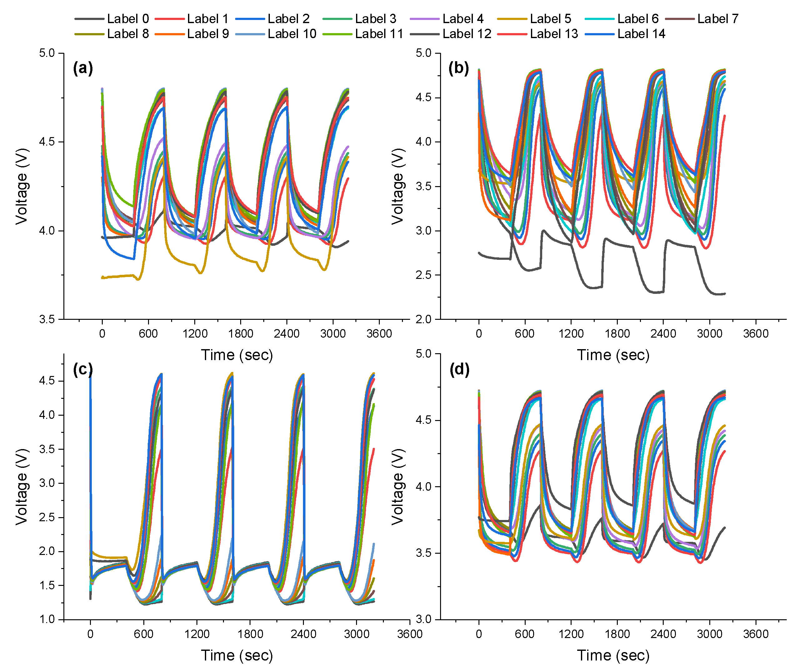
Based on the sampling rate of the sensor signals, i.e., 20 counts/s, one full cycle of gas sensing and purging constituted 16,000 data points, i.e., 8000 data points for a gas sensing time of 400 s and 8000 data points for a gas purging step of 400 s. Figure 2a–d show the whole sensor datasets acquired from four gas sensors according to the gas combinations listed in Table 1. Figure 2a–d demonstrate the sensing responses from the NOx sensor (denoted by S0), VOC sensor (denoted by S1), CO sensor (denoted by S2), and (d) alcohol sensor (denoted by S3). Each full sensor data set was composed of 16,000 data points, as shown in Figure S2 in the Supporting Material. For ANNs and DNNs, the basic set of deep learning input was assigned to 160 data points, which were periodically collected every two seconds producing 100 data sets per cycle, as shown in Figure S2b–f in the Supporting Information, where the corresponding graphs demonstrate the gas sensing information obtained from 160 points described above at the 1st, 21st, 41st, 61st, and 81st data sets (where the data sets are positioned with the interval of 0.02 s). This data sampling approach can be employed for data augmentation to overcome the limitation of data measurement sets encountered in practical sensor applications. Figure S2b–f, the data-augmented graphs based on data preprocessing, are not discernable to the naked eye. Taking into accounts the gas combinations and two cycles employed for training, a total of 3000 sets (100 × 2 × 15) were used to train the algorithms. Owing to the sampling rate of 20 counts/s, each set provided 1000 sets of data per gas combination (or equivalently gas labels) via data augmentation. After data augmentation on 15 gas labels obtained from 2 cycles, a total of 3000 sets were employed to train the deep learning algorithms, i.e., 2400 and 600 sets for training and validating the proposed algorithms, respectively. Based on one cycle of gas signals, 1500 data sets were employed for testing the proposed algorithms. The training time was ranged from several min to tens of min, which is acceptable for practical application.

3.2. Unsupervised Machine Learning: K-Means Clustering

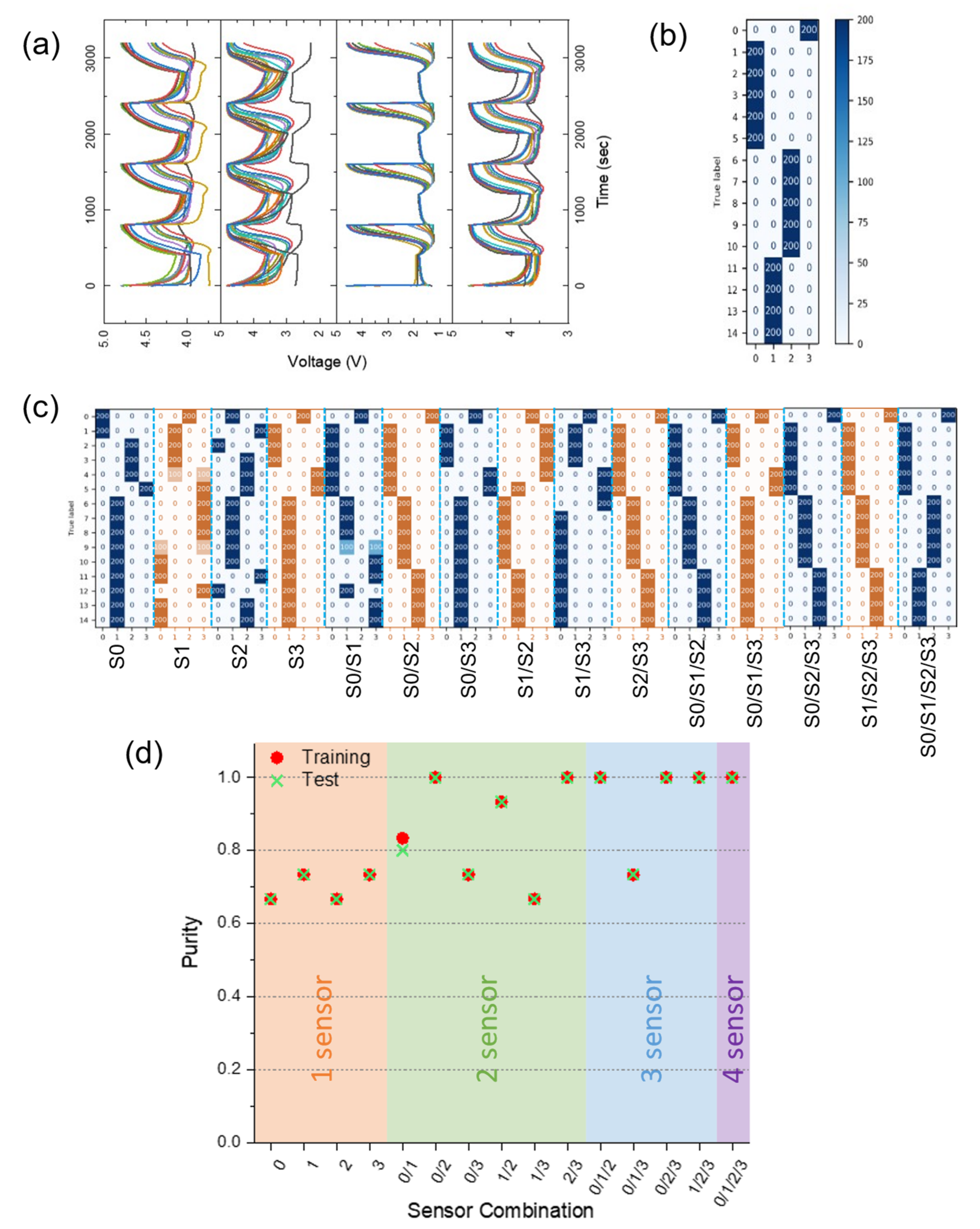
The original sensor data sets were subjected to K-means clustering, a well-known unsupervised learning technique, to evaluate the similarity among the acquired gas sensor data or between gas labels without any biased information. The number of clusters was 4, i.e., the number of gas mixture types employed in classification, i.e., N2, CO, EtOH, and CO/EtOH. Figure 3a shows the gas-sensing information plotted as a function of the gas mixture type, and Figure 3b denotes the cluster formation based on the type of gas mixture and gas combination using the 4-sensor arrays: gas mixtures are classified into four clusters, which are regrouped based on the original 15 gas combinations in Table 1. Figure 3c demonstrates the cluster formation obtained in terms of the sensor number combination. Proper cluster formations were found for the S0/S2, S2/S3, S0/S1/S2, S0/S2/S3, S1/S2/S3, and S0/S1/S2/S3 combinations. The purity function, defined by the following equation, was used to evaluate the relative belongingness of the data sets assigned to the proposed clusters:
U = i p i ( m a x j p i j p j )
where pi = ni/n, pj = nj/n, and pji = nij/n, where nij is the number of examples belonging to class i found in cluster j and ni and nj are the numbers of examples in clusters i and j, respectively [43].
As expected from Figure 3d, the purity information is excellent, with a value close to or equal to 1 in terms of gas mixture clustering. The purity was employed to evaluate the quality of the clusters obtained according to the gas mixture type and labeled gas combinations. Depending on the belongingness of the sensors, the purity ranged from 0 (impure) to 1. A purity of 1 indicates that the cluster includes labeled data from only one class. Conversely, a cluster is regarded as impure if the sensor data points belong to many different classes, leading to a low value. K-means clustering is especially advantageous in grouping data into clusters of similar gas molecule characteristics. This preliminary information can be exploited for subsequent neural network-based gas classification, which is more explicit with a high order of information to the user community. However, the proposed methodology requires further empirical and theoretical confirmation from a high volume of sensor data interpretation.

3.3. Supervised Machine Learning: Neural Network

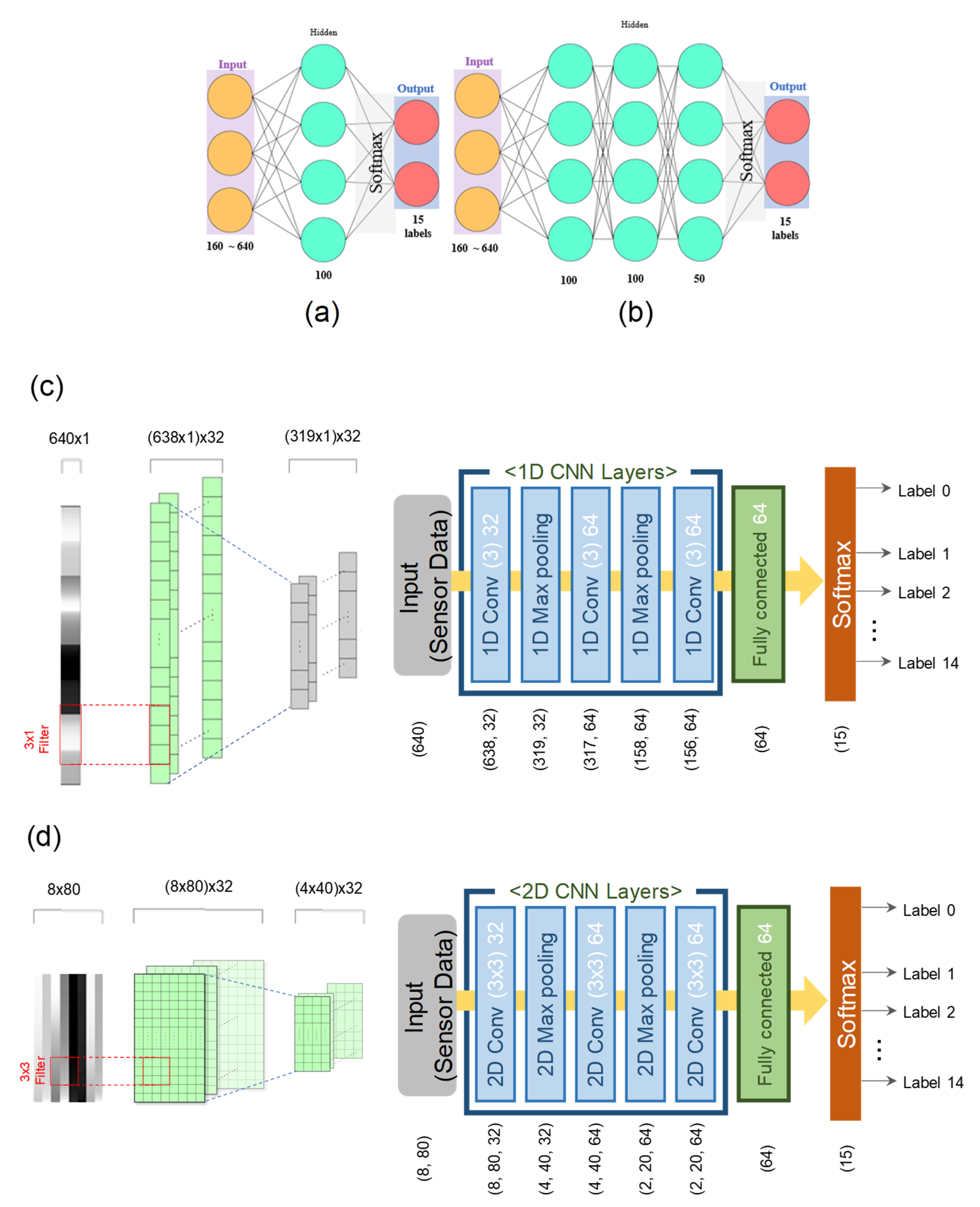
Using the data augmentation prescribed in the Experimental sections and Figure S2 in the Supporting Material, we employed a combined approach to understanding the performance of gas sensors in terms of the number of gas sensors and deep learning algorithms based on the original gas sensing information obtained from the customized 4-sensor array. The original 4-sensor data are reorganized for 1-sensor components, 2-sensor arrays, 3-sensor arrays, and 4-sensor arrays: based on the sensor number ranging from 0 to 3, the 1-sensor system constitutes the obtained data from the single sensors denoted by S0, S1, S2, and S3, treated independently. The 4-sensor system is represented by the original simultaneous measurement data acquired from concurrent measurements originating from the 4 sensors (denoted by S0/S1/S2/S3). The 2-sensor arrays include S0/S1, S0/S2, S0/S3, S1/S2, S1/S3, and S2/S3, and the 3-sensor arrays are S0/S1/S2, S0/S1/S3, S0/S2/S3, and S1/S2/S3. In addition to studying the effect of the number of sensors, we applied diverse deep learning algorithms in either numeric or image format, i.e., ANNs and DNNs for manipulating the sensor responses in numeric form and 1D CNNs and 2D CNNs for manipulating the sensor responses in image format, as illustrated in the detailed architectures of Figure 4 and Supplementary Figure S3 in the Supporting Information. The first two ANN and DNN architectures incorporated one hidden layer and three hidden layers, respectively, in addition to the ultimate output layer, which were composed of 50 or 100 neurons and incorporated filtering, and activation in the common output layers, as shown in Figure 4a,b. At the hidden layers, each node is subjected to the summation function, including all the inputs and bias, i.e., y =   ( w e i g h t i n p u t ) + b i a s and the activation function (ReLU(x) = max(x,0)). Figure 4c,d show the 1D CNN and 2D CNN: the 1D CNN employs 1D data composed of sensors repeating gas detection and gas purging; the 2D CNN data are constructed from the gas-detection signal and gas-purging information data in the different rows. As shown in Figure 4c,d, the 1D CNNs and 2D CNNs comprise 1 input layer, 3 convolutional layers with 2 max-pooling layers, and a fully connected layer followed by a softmax layer. Max pooling reduces the dimensionality in proportion to the number of input data points by performing downsampling from the preceding hidden layers. The softmax layers of the classification layer provide the final labeling information as a function of probability and the component labels (in this work, 15 labels), as defined by   f ( s i ) = exp ( s i ) / j = 1 C exp ( s j ) , where s i is the score calculated through the neural network for each class in C (C = 15). The 1D CNN applied a 3 × 1 window filter, and the 2D CNN applied a 3 × 3 window filter. Detailed information about the data formats is shown in Supplementary Figure S4 in the Supporting Materials. The above softmax functions are applied to the 1D CNN and 2D CNN approaches, in addition to the numeric-based ANN and DNN.
To optimize the deep learning algorithms, the effect of the hyperparameters on the deep learning performance was investigated in terms of the learning rate, number of neurons, and batch size, especially for the 4-sensor ANNs because there has been no report on these elementary issues, despite the basic checkpoints for the deep learning methodology and the significant roles of the parameters chosen. In this work, the learning rate was set to 0.01 for time- and performance-wise approaches: Figure S5 in the Supporting Information shows the training and validation optimization based on the accuracy and loss with the learning rate varying from 10−1 to 10−3. When the number of neurons in the hidden layer was 50, 100, and 200, there were no detectable changes in the corresponding accuracies and losses (see Figure S6 in the Supporting Information). The current neural networks employed 100 neurons. Last, the batch size was varied among 16, 32, 64, or 128. The smaller the batch size is, the longer the training time. The larger the batch size is, the greater the computational load. If the batch size is small, local minima can be avoided, leading to the global minimum and resulting in a longer training time. Conversely, if the batch size is large, the computational load becomes considerable, and the result sometimes remains at a local minima. Therefore, the batch size was set to 32 (see Figure S7 in the Supporting Information). The corresponding accuracies and losses were calculated at epoch 1000. Depending on the neural network architectures, the number of weights and biases vary significantly, as demonstrated in Supplementary Table S1. Image-based convolutional networks (1D CNN and 2D CNN) require much higher numbers of parameters than those based on numeric-based ANN and DNN. The 1D CNN architecture involved 167,183, 331,023, 494,863, and 658,703 parameters for the 1-sensor, 2-sensor, 3-sensor, and 4-sensor combination modes, respectively. Contrary to 1D CNN, the ANN architecture requires a smaller number of parameters at 17,615, 33,615, 49,615 and 65,615 for the 1-sensor, 2-sensor, 3-sensor, and 4-sensor combination modes, respectively.
Accuracy, recall, precision, and loss were employed to evaluate the performance of the proposed model or algorithm for gas classification. The loss values were calculated using cross entropy.
Accuracy = (TP + TN)/(TP + FP + TN + FN)
Recall = TP/(TP + FN)
Precision = TP/(TP + FP)
Loss ( Cross   entropy ) = i C t i log ( f ( s i ) )
where TP denotes true positive, TN denotes true negative, FP denotes false positive, FN denotes false negative, and ti denotes the ground truth score for each class (i) in C. A confusion matrix was employed to assess the gas sensing/labeling. Almost all the gas labeling results were in excellent agreement with the ground truth data information. Taking into accounts that 100 data sets were labeled for each class tested, the highest counts of ‘100′ assigned along the matrix diagonal indicates that the corresponding deep learning model accurately detected the targeted gas combination (see Figure S8 in the Supporting Material for the deep learning-based predictions in the 4-layered DNN and 1D CNN algorithms).
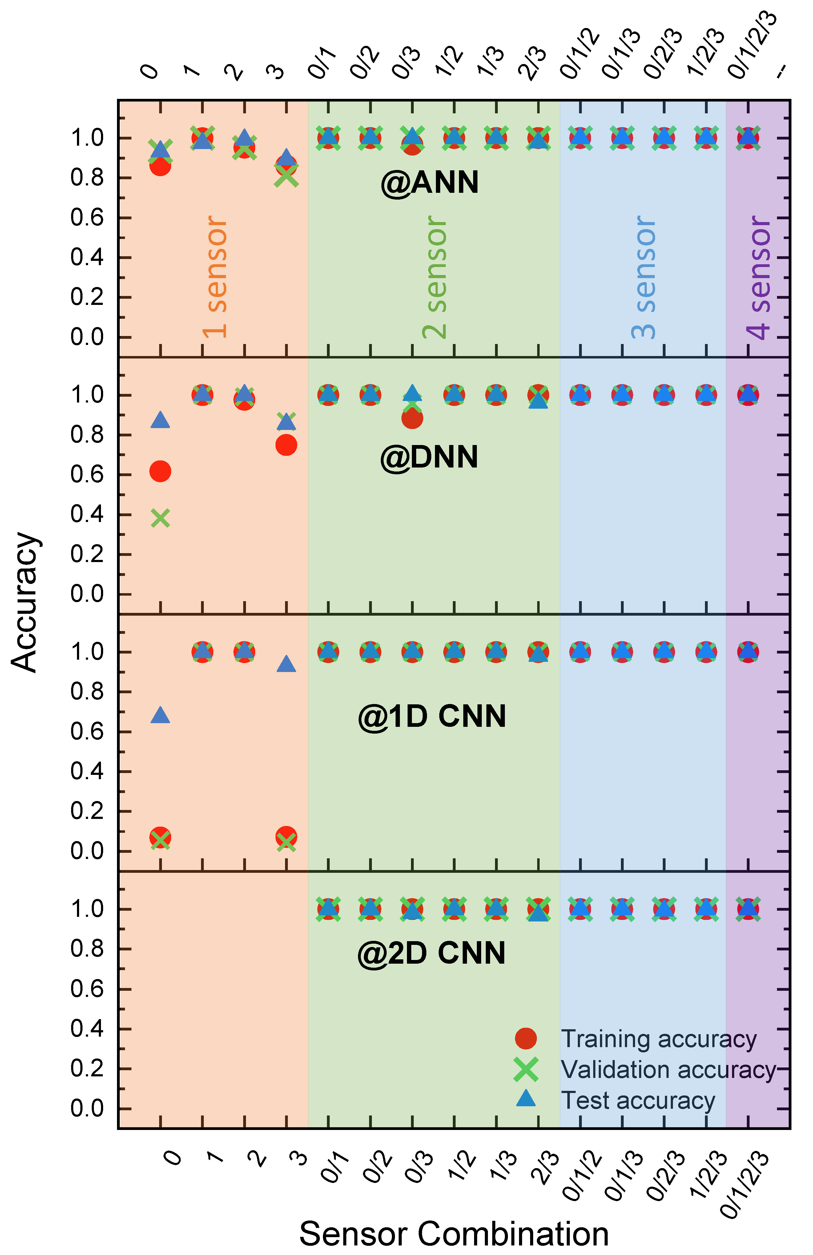
Supplementary Figures S9 and S10 in the Supporting Information illustrate the effect of the sensor combination on deep learning-based predictions in the 4-layered DNN and 1D CNN algorithms, along with the detailed numerical values (provided in Supplementary Tables S2–S5). Two sensors, S1 and S2, were key to classifying the gas labeling information, as concluded from the results of the single sensors and multiple sensor combinations. As evidenced in the paired accuracy and loss information obtained as a function of epoch, the accuracy converges to approximately 1. The deep learning-based effectiveness was evaluated based on the accuracy and loss and their fluctuating responses. In particular, image data converted from numeric data were most effective in terms of deep learning performance. Generally, the greater the number of sensors in a multiple sensor array, the more accurate the deep learning-based predictions. Nonetheless, a small number of key component sensors, S1 and S2, were identified. The two-sensor combination of S1 and S2 performed similarly to the 4-sensor arrays. Additionally, the S1/S2/S3 and S0/S1/S2 combinations performed well. Notably, poor performance was observed for most single sensors. In particular, the inferior features were found in the 1D CNN algorithms, and the similar finding was obtained for the 4-layered DNN algorithms.
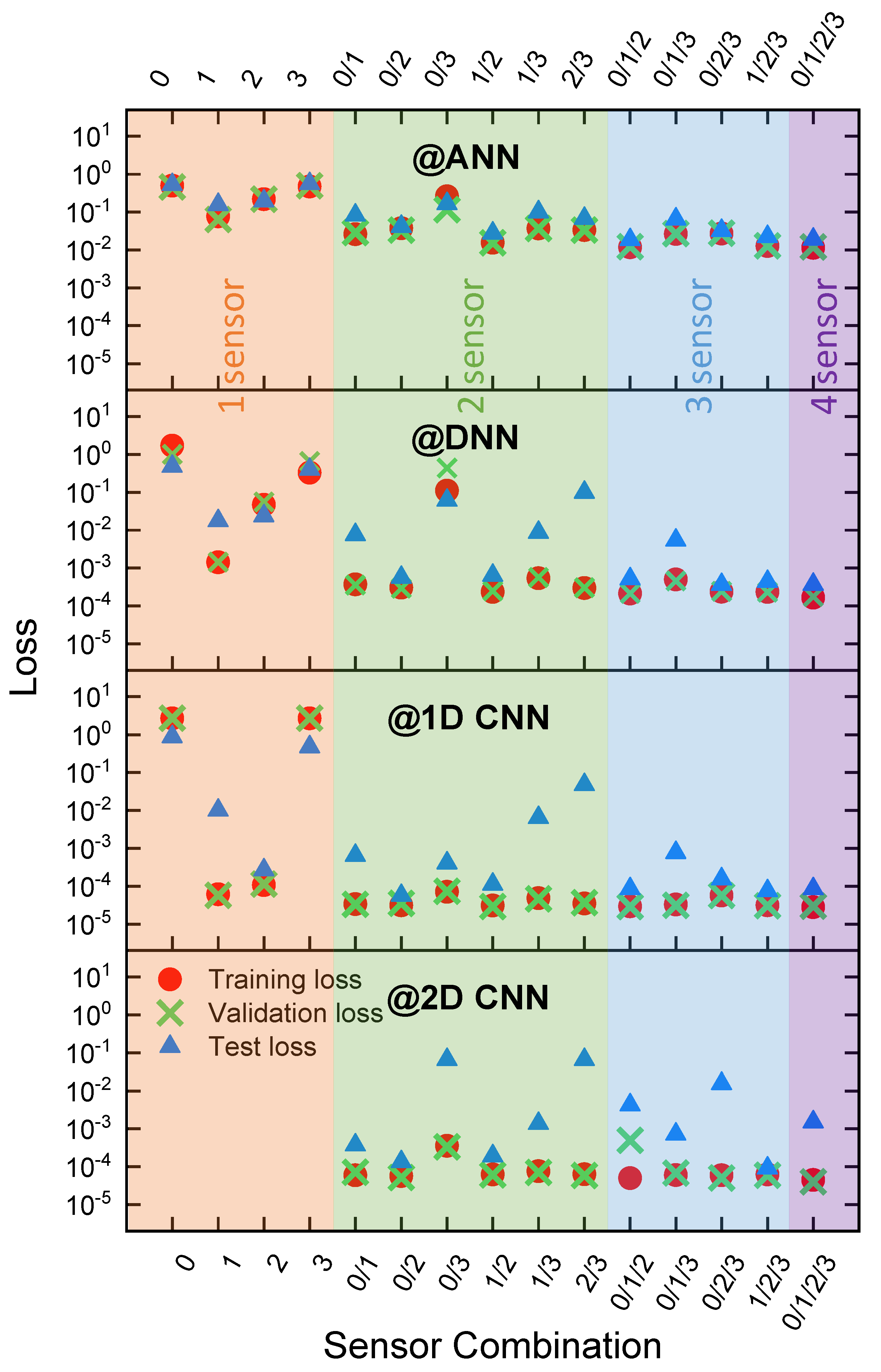
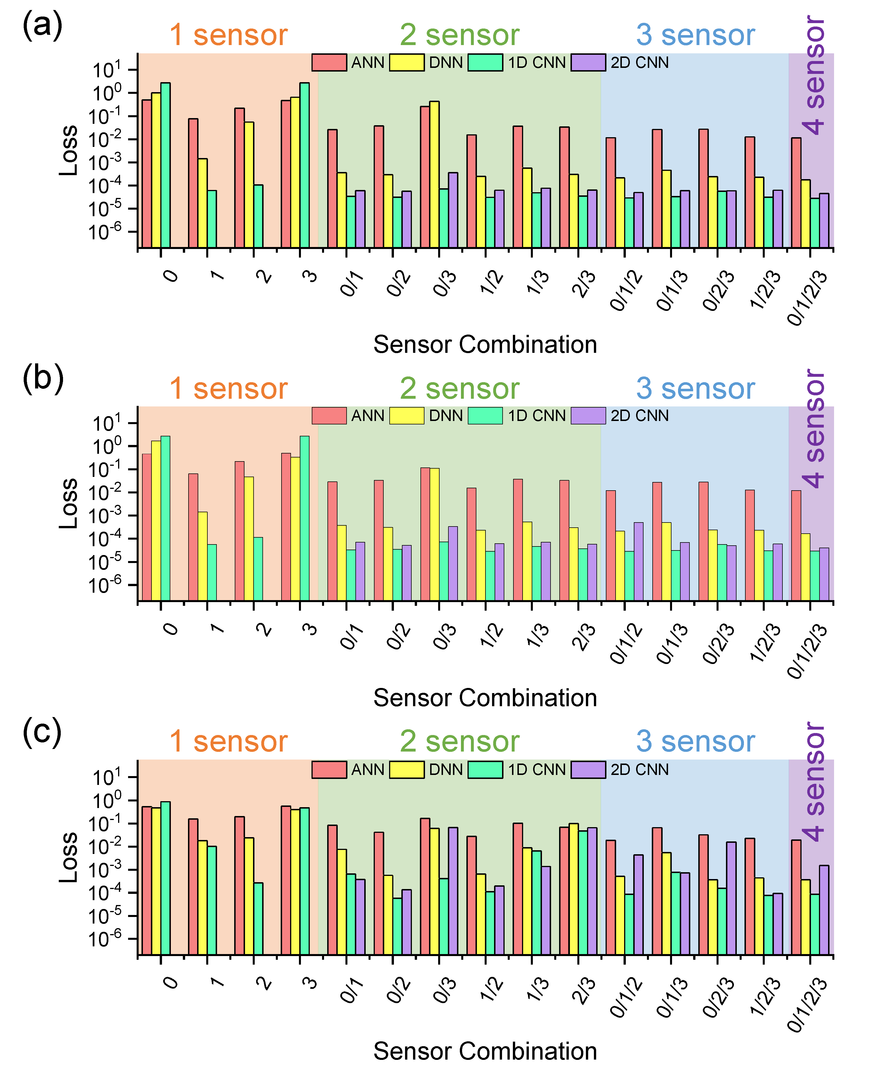
Figure 5 and Figure 6 exhibit the accuracy and loss information obtained through the application of ANN, DNN, 1D CNN and 2D CNN in the training, validation, and test stages for gas sensors in terms of 15 gas combination labels collected from 4-sensor array systems. For comparison, the minimum epoch was extracted for the specific loss value, i.e., 0.01 during the application of deep learning tools to gas sensor labeling, with special emphasis on two parameters, i.e., accuracy and loss. Image-based labeling methods, i.e., 1D CNN and 2D CNN, outperformed the 2-layer ANN and 4-layer DNN, which incorporate numeric-based inputs, demonstrating much lower losses at the fixed epoch, as shown in Supplementary Tables S2–S5: the CNN architecture is attributed to the higher feature-capturing capability from image-data format, unlike the simplified mathematical calculation based on the numeric data format in ANNs and DNNs. Furthermore, the DNN outperformed the ANN, due to the higher number of parameters in DNNs because the DNN includes 3 hidden layers whereas the ANN includes a single layer. The gas sensing data reflect the nonlinearity between variables (or, equivalently, neurons). Imperfectness of the neurons or variables (or weights), is observed in the 2-layer ANN; however, the addition of the hidden layer enhances the prediction capability of the 4-layered DNN architectures by increasing the variables (or weights).
Unsupervised machine learning methodologies have been reported widely: Banerjee et al. performed clustering of 400 black tea datasets [44] using PCA, and K-means clustering was applied to the clustering of indoor air quality analysis by setting K to 2 to 10 [40]. There have been recently reported deep learning-based applications involving diverse neural networks [19,35,45,46,47,48,49,50]. Kumar et al. applied two-layered artificial neural networks to gas sensor array drift datasets, leading to the classification of six pollutant gases with an accuracy of 86.77% [45]. Peng et al. employed convolutional neural networks made up of six convolutional block and three max pooling layers to classify four gases, leading to an accuracy of 95.2% and reported the benefits of the deep learning-based DCCN against support vector machine (SVM) and multilayer perceptron (MLP) with emphasis on methodology for gas classification [34]. Chu et al. used two-dimensional convolutional neural networks to classify 11 gas combinations composed of NO2 and CO gases, and obtained a deep learning accuracy of 94.55% [46]. Unlike previous works, recurrent neural networks were chosen to classify time-dependent gas information obtained from four different gas species, achieving an accuracy of 82% [47]. Chen et al. incorporated mixed-kernel variable-dimension memristive convolutional neural networks for electronic nose applications, i.e., one-dimensional CNNs and two-dimensional CNNs, which obtained accuracies of 98.75% and 98.61%, respectively [48]. For deep learning-based applications, the data inputs employed were grouped into two types, i.e., from the gas sensing transient [34] and from both the gas sensing transient and gas purge transient [46,49,50] in the neural networks, including ANNs and CNNs. There is limited information on direct comparison between numeric- and image-based approaches combined with appropriate data augmentation in terms of sensor combinations. Cho et al. applied the neural-network based approach, i.e., gated recurrent unit (GRU)-based autoencoders to metallic gas sensors, which enabled detection of hidden signals in sensors targeting at hydrogen gas species. Ref. [51] Yaqoob and Younis reviewed diverse gas sensors operating on chemresistive and FET features along with the potential of machine learning. Ref. [52] Kang et al. combined a batch-uniform fabrication strategy in SMO sensors with neural networks, CNN (convolutional neural networks), leading to high accuracy in real-time gas detection. Ref. [53] Kanaparth and Singh employed temperature-dependent comparisons of a single ZnO sensor with diverse machine learning techniques, i.e., Naïve Bayes, Support Vector Machine, Random Forest, and Logistic Regression classifiers [54]. In our work, we adopted neural network-based DNNs and 1-D CNNs in terms of numeric and image-based input format, respectively. Despite the simplicity of neural networks, the machine learning performance is proven to be significant by proposing the minimum number of sensors with the aim of discriminating the harmful gas species enough to cope with the real-time monitoring against harmful environments. The two-sensor combination can be exploited under hostile environments composed of harmful gas species. In contrast to previous work, this work focused on diverse types of deep learning algorithms and various numbers of sensors, which exploits the novel data augmentation strategy (of Supplementary Figure S2) and the simplified deep learning architectures (i.e., the number of hidden layers in DNNs and the number of convolutional layers in 1D CNNs and 2D CNNs) as shown in Figure 4 and Supplementary Figure S3. The greater the sensor number is, the better the classification performance. However, some single sensors and combinations of two or three sensors achieve good deep-learning performance almost equivalent to that achieved with the maximum number of sensors. The current approach employs different deep learning methods to conduct gas mixture labeling through a model experimental design, i.e., the input data formats can be numeric values, images, or time-dependent numeric values. CNN architectures were developed for image classification. Traditionally, CNNs were optimized to 2D CNNs for feature engineering. Moreover, a CNN can be adjusted to a 1D image, where sequential data are provided in a fixed length segment format. The 1D CNN can be exploited for deep learning with chemical gas sensors. Through the synergistic combination of K-Means clustering and neural network-based deep learning, a method for gas detection/classification is proposed for choosing the optimized sensor environment in support with machine learning, i.e., neural network-based schemes.
As demonstrated in Figure 6 and Figure 7, the presence of the high-selectivity sensors, i.e., sensors S1 and S2, enhances the prediction performance. The performances of the 1D CNN and 2D CNN are quite similar in the training and test stages. The 1D CNN is optimized for the current time-sequential sensing voltage-based gas sensing application. Based on the deep learning performance of Figure 5 and Figure 6, a relative ranking can be assigned to the sensor combinations employed for machine learning in Supplementary Tables S6–S8, showing that two superior sensors are sufficient for high-performance gas sensing/labeling; however, note that the greater the number of sensors employed for detection, the better the classification accuracy achieved by the deep learning algorithms. In addition to the optimized sensor combination, the different sensor combinations can be usefully exploited to cross-check the sensor performance periodically and/or artificially. The sensor combination performance table (as shown in Supplementary Tables S6–S8) will be proposed as a reference data sheet for practical monitoring tasks, even if a whole defect-free sensor combination is preferred for ideal sensing operations. In other words, we need a sensor replacement list for unexpected failures encountered in operation sites, i.e., out of order, malfunction, and degradation.
The current work aims to provide an elementary understanding of the application of deep learning to gas sensing labeling based on analog voltage signals (or resistances) obtained as a function of time. Although the gas combination and gas sensing of a multiarray sensor system is chosen as a model system, the confusion matrix is shown to be free from errors in deep learning-inferred predictions. The current work presented the unique features capable of expanding machine learning to sensor domains: (i) a data augmentation methodology that exploits high-sampling rate (20 points/sec) sensing data for high-volume deep learning management by producing many useful datasets for training, validation, and testing procedures; (ii) a machine learning approach that incorporates complementary K-Means clustering and neural network-based deep learning and confirms their performances of machine learning methodologies (four clusters in K-Means clustering vs. neural network-assisted gas discrimination (15 labels); and (iii) a systematic approach and supplementary information for optimized sensor combination for a super-sensor combination (which can provide the highest machine learning by adopting the minimized number of sensors instead of the unlimited full sensor configuration) combination instead of the whole sensor combination, (for example the two-sensor combination recommended can be exploited for the practical machine learning-assisted discrimination).
Future works will cover more challenging applications that incorporate the influence of degradation and the effect of relative humidity and/or time-dependent degradation on sensor performance, in addition to the applicability of unsupervised learning. Sensitivity, selectivity, and stability are essential issues to address in semiconductor sensors, in addition to response time, recovery time, and cost. The current work demonstrates that the effectively designed interactive sensor arrays can be exploited for superior performance, which includes high sensitivity, high selectivity, high stability, low response time and recovery time with low cost.

4. Conclusions

Machine learning-based classification was applied to gas sensing with the multiple SMO gas sensors as a function of mixtures of carbon monoxide and ethyl alcohol. The 4-sensor configuration data were subdivided into 3-, 2-, and 1-sensor formats to assess the effect of the number of sensors on deep learning-based predictions. The similarity features between data sets were clustered successfully using K-means clustering based on the chemical traits in direct association with the voltage responses to detect gas species. The sensor configuration format was combined with the counterpart of deep learning-based prediction algorithms, i.e., ANNs, DNNs, 1-D CNNs, and 2-D CNNs. The high data sampling rate allows for data augmentation, which is a prerequisite when exploiting deep learning algorithms based on supervised learning. The gas labeling capability ranked as follows: 1D CNN, 2D CNN, DNN, and ANN. Based on the accuracy and loss information, the respective validation indicates that the interactive features of semiconductor-type gas sensors can be exploited as fingerprints for gas classification (or labeling). The inherent disadvantages of chemical sensors can be synergistically employed to recognize hidden patterns that are not easily recognized by humans. By analyzing the effect on the proposed sensor combination on gas detection/classification performance based on the complete gas response data obtained from the gas sensing and gas purge transients, it is demonstrated that this optimized sensor combination can be implemented via deep learning algorithms for practical applications requiring high-performance gas detection/classification tasks. Since the current work was performed under the well-controlled gas sensing environment, the upcoming machine learning should probe the prediction capability encountered in application domains, along with the sensor-to-sensor variation and degradation issues.

Supplementary Materials

The following supporting information can be downloaded at: https://www.mdpi.com/article/10.3390/electronics11233884/s1, Figure S1: (a) Gas sensing data acquisition system for machine learning obtained from a gas sensor array system involving software-controlled gas mixture combinations. (b) Schematic description on gas sensing data sets acquired by the gas sensing data acquisition system for machine learning. (One full cycle is composed of gas sensing and gas purge transients.); Figure S2: Data preprocessing for deep learning analysis applied to gas sensing applications. (a) The original graph using 16,000 points, (b) the graph using 160 points selected from the first group, (c) the graph using 160 points selected from the 21th group, and (d) the graph that incorporates 160 points from the 41th point, (e) the graph using 160 points selected from the 61th group, and (f) the graph that incorporates 160 points from the 81th point. Figure S3: Detailed deep learning architectures employed for (a) 1D CNN and 2D CNN. Figure S4: Gas sensing data input formats subjected to deep learning algorithms for gas sensor classification, i.e., ANN, DNN, 1D CNN, 2D CNN, and RNN. (a) 1 sensor, (b) 2 sensors, (c) 3 sensors, and (d) four. Figure S5: Effect of learning rate on the training and validation performance of the 4-sensor DNN algorithm, monitored in terms of the accuracy and loss functions. (a) & (b) Accuracy and loss functions in the training stage and (c) & (d) accuracy and loss functions obtained from the validation stage. Figure S6: Effect of the number of neurons in the hidden layer on the training and validation performance of the 4-sensor DNN algorithm, monitored in terms of the accuracy and loss functions. (a) & (b) Accuracy and loss functions in the training stage and © & (d) accuracy and loss functions obtained from the validation stage. Figure S7: Effect of batch size on the training and validation performance in the 4-sensor DNN algorithm, monitored in terms of the accuracy and loss functions. (a) & (b) Accuracy and loss functions in the training step and (c) & (d) accuracy and loss functions obtained from the validation stage. Figure S8: Exemplary confusion matrix obtained from the deep learning-based predictions for gas sensor classification using the (a) 4-layered DNN and (b) 1D CNN algorithms in the S0/S1/S2/S3 combination mode. Figure S9: Example analysis information for the (a) accuracy and (b) loss functions obtained from the application of the 4-layer DNN algorithm to CO/C2H5OH-based gas detection/classification. Figure S10: Example analysis information for the (a) accuracy and (b) loss functions obtained from the application of the 1D CNN algorithm to CO/C2H5OH-based gas detection/classification. Table S1: Information on the total number of neural network weights and biases according to neural network architectures employed for the application of 4 sensor array system to machine learning-based gas detection/classification. Table S2. Deep learning performance as a function of gas sensor combinations in the training, validation, and test stages based on the 2-layer ANN algorithm (calculated at 1,000 epochs). Table S3. Deep learning performance as a function of gas sensor combinations in the training, validation, and test stages based on the 4-layered DNN algorithm (calculated at 1,000 epochs). Table S4. Deep learning performance as a function of gas sensor combinations in the training, validation, and test stages based on the 1D CNN algorithm (calculated at 1,000 epochs). Table S5. Deep learning performance as a function of gas sensor combinations in the training, validation, and test stages based on the 2D CNN algorithm (calculated at 1,000 epochs). Table S6. Ranking information based on accuracy and loss statistics (at 1,000 epochs) at training phases obtained from the application of ANN, DNN, 1D-CNN, and 2D-CNN to gas detection/classification. (Notes that the priority is given to the lowest loss values in the cases where the accuracies are equal. Table S7. Ranking information based on accuracy and loss statistics (at 1,000 epochs) at validation phases obtained from the application of ANN, DNN, 1D-CNN, and 2D-CNN to gas detection/classification. (Notes that the priority is given to the lowest loss values in the cases where the accuracies are equal. Table S8. Ranking information based on accuracy and loss statistics (at 1,000 epochs) at test phases obtained from the application of ANN, DNN, 1D-CNN, and 2D-CNN to gas detection/classification. (Notes that the priority is given to the lowest loss values in the cases where the accuracies are equal.

Author Contributions

Conceptualization, J.-O.L., K.-S.A. and Y.Y.; methodology, Y.N.; software, M.-I.L.; validation, M.-J.L. and W.K.; formal analysis, J.O. and H.H.; investigation, J.O.; resources, H.-W.S.; data curation, S.S.P.; writing—original draft preparation, Y.Y., J.L. and J.-H.H.; writing—review and editing, Y.Y., J.L. and J.-H.H.; visualization, J.O. and Y.N. supervision, J.-H.H.; project administration, J.-H.H.; funding acquisition, J.-H.H. All authors have read and agreed to the published version of the manuscript.

Funding

This research was supported by (New Project Breath Sensors) Nano Material Technology Development Program through the National Research Foundation of Korea (NRF) funded by Ministry of Science and ICT (NRF No. 2021M3H4A3A02086452), by the MSIT (Ministry of Science and ICT) Korea, under the Basic Science Research Programs through the National Research Foundation of Korea (NRF) (2020R1F1A104826411), by the National Research Foundation of Korea (NRF) grant funded by the Korea government (MSIT) (NRF-2022R1F1A1074526), and by the Ministry of Trade, Industry & Energy (MOTIE) and the Korea Institute for Advancement of Technology (KIAT), under Grants P0014268 Smart HVAC demonstration support.

Data Availability Statement

The raw data required to reproduce these findings cannot be shared at this time, as the data also form part of an ongoing study. The data are available from the corresponding author upon reasonable request.

Acknowledgments

All individuals included in this section have consented to the acknowledgement.

Conflicts of Interest

The authors declare no conflict of interest.

References

  1. Dey, A. Semiconductor metal oxide gas sensors: A review. Mater. Sci. Eng. B 2018, 229, 206–217. [Google Scholar] [CrossRef]
  2. Yeo, J.; Lim, C. Emerging flexible and wearable physical sensing platforms for healthcare and biomedical applications. Microsyst. Nanoeng. 2016, 2, 1–19. [Google Scholar] [CrossRef] [Green Version]
  3. Zhu, L.; Zeng, W. Room-temperature gas sensing of ZnO-based gas sensor: A review. Sens. Actuators A Phys. 2017, 267, 242–261. [Google Scholar] [CrossRef]
  4. Patel, S.; Park, H.; Bonato, P.; Chan, L.; Rodgers, M. A review of wearable sensors and systems with application in rehabilitation. J. Neuroeng. Rehabil. 2012, 9, 21. [Google Scholar] [CrossRef] [PubMed] [Green Version]
  5. Tanaka, M. An industrial and applied review of new MEMS devices features. Microelectron. Eng. 2007, 84, 1341–1344. [Google Scholar] [CrossRef]
  6. Yamazoe, N.; Shimanoe, K. New perspectives of gas sensor technology. Sens. Actuators B Chem. 2009, 138, 100–107. [Google Scholar] [CrossRef]
  7. Bhattacharyya, P. Technological journey towards reliable microheater development for MEMS gas sensors: A review. IEEE Trans. Device Mater. Reliab. 2014, 14, 589–599. [Google Scholar] [CrossRef]
  8. Hsieh, Y.C.; Yao, D.J. Intelligent gas-sensing systems and their applications. J. Micromech. Microeng. 2018, 28, 093001. [Google Scholar] [CrossRef]
  9. He, J.; Xu, L.; Wang, P.; Wang, Q. A high precise E-nose for daily indoor air quality monitoring in living environment. Integration 2017, 58, 286–294. [Google Scholar] [CrossRef]
  10. Bieganowski, A.; Jaromin-Glen, K.; Guz, Ł.; Łagód, G.; Jozefaciuk, G.; Franus, W.; Suchorab, Z.; Sobczuk, H. Evaluating soil moisture status using an e-nose. Sensors 2016, 16, 886. [Google Scholar] [CrossRef] [PubMed]
  11. Zeng, H.; Takahashi, T.; Kanai, M.; Zhang, G.; He, Y.; Nagashima, K.; Yanagida, T. Long-term stability of oxide nanowire sensors via heavily doped oxide contact. ACS Sens. 2017, 2, 1854–1859. [Google Scholar] [CrossRef] [PubMed]
  12. Wang, C.; Yin, L.; Zhang, L.; Xiang, D.; Gao, R. Metal oxide gas sensors: Sensitivity and influencing factors. Sensors 2010, 10, 2088–2106. [Google Scholar] [CrossRef] [Green Version]
  13. Geng, B.; Fang, C.; Zhan, F.; Yu, N. Synthesis of polyhedral ZnSnO3 microcrystals with controlled exposed facets and their selective gas-sensing properties. Small 2008, 4, 1337–1343. [Google Scholar] [CrossRef] [PubMed]
  14. Persaud, K.; Dodd, G. Analysis of discrimination mechanisms in the mammalian olfactory system using a model nose. Nature 1982, 299, 352–355. [Google Scholar] [CrossRef]
  15. Karakaya, D.; Ulucan, O.; Turkan, M. Electronic nose and its applications: A survey. Int. J. Autom. Comput. 2020, 17, 179–209. [Google Scholar] [CrossRef] [Green Version]
  16. Guntner, A.T.; Koren, V.; Chikkadi, K.; Righettoni, M.; Pratsinis, S.E. E-nose sensing of low-ppb formaldehyde in gas mixtures at high relative humidity for breath screening of lung cancer? ACS Sens. 2016, 1, 528–535. [Google Scholar] [CrossRef]
  17. Haugen, J.E.; Kvaal, K. Electronic nose and artificial neural network. Meat Sci. 1998, 49, S273–S286. [Google Scholar] [CrossRef]
  18. Brudzewski, K.; Osowski, S.; Markiewicz, T. Classification of milk by means of an electronic nose and SVM neural network. Sens. Actuators B Chem. 2004, 98, 291–298. [Google Scholar] [CrossRef]
  19. Benedetti, S.; Mannino, S.; Sabatini, A.G.; Marcazzan, G.L. Electronic nose and neural network use for the classification of honey. Apidologie 2004, 35, 397–402. [Google Scholar] [CrossRef] [Green Version]
  20. Rocha, L.A.; Dias, R.A.; Cretu, E.; Mol, L.; Wolffenbuttel, R.F. Auto-calibration of capacitive MEMS accelerometers based on pull-in voltage. Microsyst. Technol. 2011, 17, 429–436. [Google Scholar] [CrossRef]
  21. Liu, H.; Li, Q.; Yan, B.; Zhang, L.; Gu, Y. Bionic electronic nose based on MOS sensors array and machine learning algorithms used for wine properties detection. Sensors 2018, 19, 45. [Google Scholar] [CrossRef] [Green Version]
  22. Wei, G.; Li, G.; Zhao, J.; He, A. Development of a LeNet-5 gas identification CNN structure for electronic noses. Sensors 2019, 19, 217. [Google Scholar] [CrossRef] [Green Version]
  23. Capone, S.; Epifani, M.; Quaranta, F.; Siciliano, P.; Taurino, A.; Vasanelli, L. Monitoring of rancidity of milk by means of an electronic nose and a dynamic PCA analysis. Sens. Actuators B Chem. 2001, 78, 174–179. [Google Scholar] [CrossRef]
  24. Tian, X.Y.; Cai, Q.; Zhang, Y.M. Rapid classification of hairtail fish and pork freshness using an electronic nose based on the PCA method. Sensors 2011, 12, 260–277. [Google Scholar] [CrossRef] [Green Version]
  25. Mahmodi, K.; Mostafaei, M.; Mirzaee-Ghaleh, E. Detection and classification of diesel-biodiesel blends by LDA, QDA and SVM approaches using an electronic nose. Fuel 2019, 258, 116114. [Google Scholar] [CrossRef]
  26. Liao, Y.H.; Wang, Z.C.; Zhang, F.G.; Abbod, M.F.; Shih, C.H.; Shieh, J.S. Machine learning methods applied to predict ventilator-associated pneumonia with Pseudomonas aeruginosa infection via sensor array of electronic nose in intensive care unit. Sensors 2019, 19, 1866. [Google Scholar] [CrossRef] [PubMed] [Green Version]
  27. Yang, J.; Sun, Z.; Chen, Y. Fault detection using the clustering-kNN rule for gas sensor arrays. Sensors 2016, 16, 2069. [Google Scholar] [CrossRef] [PubMed] [Green Version]
  28. Xu, L.; Yu, X.; Liu, L.; Zhang, R. A novel method for qualitative analysis of edible oil oxidation using an electronic nose. Food Chem. 2016, 202, 229–235. [Google Scholar] [CrossRef]
  29. Goodner, K.L.; Dreher, J.G.; Rouseff, R.L. The dangers of creating false classifications due to noise in electronic nose and similar multivariate analyses. Sens. Actuators B Chem. 2001, 80, 261–266. [Google Scholar] [CrossRef]
  30. Ren, Y.; Ramaswamy, H.S.; Li, Y.; Yuan, C.; Ren, X. Classification of impact injury of apples using electronic nose coupled with multivariate statistical analyses. J. Food Process Eng. 2018, 41, e12698. [Google Scholar] [CrossRef]
  31. Aguilera, T.; Lozano, J.; Paredes, J.A.; Alvarez, F.J.; Suárez, J.I. Electronic nose based on independent component analysis combined with partial least squares and artificial neural networks for wine prediction. Sensors 2012, 12, 8055–8072. [Google Scholar] [CrossRef]
  32. Giungato, P.; Laiola, E.; Nicolardi, V. Evaluation of industrial roasting degree of coffee beans by using an electronic nose and a stepwise backward selection of predictors. Food Anal. Methods 2017, 10, 3424–3433. [Google Scholar] [CrossRef]
  33. Baskar, C.; Nesakumar, N.; Rayappan, J.B.B.; Doraipandian, M. A framework for analysing E-Nose data based on fuzzy set multiple linear regression: Paddy quality assessment. Sens. Actuators A Phys. 2017, 267, 200–209. [Google Scholar] [CrossRef]
  34. Peng, P.; Zhao, X.; Pan, X.; Ye, W. Gas classification using deep convolutional neural networks. Sensors 2018, 18, 157. [Google Scholar] [CrossRef] [Green Version]
  35. Zhao, X.; Wen, Z.; Pan, X.; Ye, W.; Bermak, A. Mixture gases classification based on multi-label one-dimensional deep convolutional neural network. IEEE Access 2019, 7, 12630–12637. [Google Scholar] [CrossRef]
  36. Chen, Z.; Chen, Z.; Song, Z.; Ye, W.; Fan, Z. Smart gas sensor arrays powered by artificial intelligence. J. Semicond. 2019, 40, 111601. [Google Scholar] [CrossRef]
  37. Jiang, P.; Hu, Z.; Liu, J.; Yu, S.; Wu, F. Fault diagnosis based on chemical sensor data with an active deep neural network. Sensors 2016, 16, 1695. [Google Scholar] [CrossRef] [Green Version]
  38. Liu, Q.; Hu, X.; Ye, M.; Cheng, X.; Li, F. Gas recognition under sensor drift by using deep learning. Int. J. Intell. Syst. 2015, 30, 907–922. [Google Scholar] [CrossRef]
  39. Ahn, J.; Shin, D.; Kim, K.; Yang, J. Indoor air quality analysis using deep learning with sensor data. Sensors 2017, 17, 2476. [Google Scholar] [CrossRef] [Green Version]
  40. Caron, A.; Redon, N.; Coddeville, P.; Hanoune, B. Identification of indoor air quality events using a K-means clustering analysis of gas sensors data. Sens. Actuators B Chem. 2019, 297, 126709. [Google Scholar] [CrossRef]
  41. Pedregosa, F.; Varoquaux, G.; Gramfort, A.; Michel, V.; Thirion, B.; Grisel, O.; Blondel, M.; Prettenhofer, P.; Weiss, R.; Dubourg, V.; et al. Scikit-learn: Machine learning in Python. J. Mach. Learn. Res. 2011, 12, 2825–2830. Available online: https://scikit-learn.org/stable/ (accessed on 10 November 2011).
  42. GitHub. Available online: https://github.com/fchollet/keras (accessed on 8 October 2019).
  43. Palacio-Niño, J.O.; Berzal, F. Evaluation metrics for unsupervised learning algorithms. arXiv 2019, arXiv:1905.05667. [Google Scholar] [CrossRef]
  44. Banerjee, M.B.; Roy, R.B.; Tudu, B.; Bandyopadhyay, R.; Bhattacharyya, N. Black tea classification employing feature fusion of E-Nose and E-Tongue responses. J. Food Eng. 2019, 244, 55–63. [Google Scholar] [CrossRef]
  45. Kumar, J.R.R.; Pandey, R.K.; Sarkar, B.K. Pollutant gases detection using the machine learning on benchmark research datasets. Procedia Comput. Sci. 2019, 152, 360–366. [Google Scholar] [CrossRef]
  46. Chu, J.; Li, W.; Yang, X.; Wu, Y.; Wang, D.; Yang, A.; Yuan, H.; Wang, X.; Li, Y.; Rong, M. Identification of gas mixtures via sensor array combining with neural networks. Sens. Actuators B Chem. 2021, 329, 129090. [Google Scholar] [CrossRef]
  47. Narkhede, P.; Walambe, R.; Mandaokar, S.; Chandel, P.; Kotecha, K.; Ghinea, G. Gas detection and identification using multimodal artificial intelligence based sensor fusion. Appl. Syst. Innov. 2021, 4, 3. [Google Scholar] [CrossRef]
  48. Chen, J.; Wang, L.; Duan, S. A mixed-kernel, variable-dimension memristive CNN for electronic nose recognition. Neurocomputing 2021, 461, 129–136. [Google Scholar] [CrossRef]
  49. Han, L.; Yu, C.; Xiao, K.; Zhao, X. A new method of mixed gas identification based on a convolutional neural network for time series classification. Sensors 2019, 19, 1960. [Google Scholar] [CrossRef] [Green Version]
  50. Chu, J.; Li, W.; Yang, X.; Yu, H.; Wang, D.; Fan, C.; Yang, A.; Li, Y.; Wang, X.; Rong, M. Quantitative detection of mixed gases by sensor array using c-means clustering and artificial neural network. In Proceedings of the IECON 2019-45th Annual Conference of the IEEE Industrial Electronics Society, Lisbon, Portugal, 14–17 October 2019; IEEE: Piscataway, NJ, USA, 2019; pp. 6748–6751. [Google Scholar] [CrossRef]
  51. Cho, S.; Lee, Y.; Lee, S.; Kang, H.; Kim, J.; Choi, J.; Ryu, J.; Joo, H.; Jung, H.; Kim, J. Finding Hidden Signals in Chemical Sensors Using Deep Learning. Anal. Chem. 2020, 92, 6529–6537. [Google Scholar] [CrossRef]
  52. Yaqoob, U.; Younis, M. Chemical gas sensors: Recent developments, challenges, and the potential of machine learning—A review. Sensors 2021, 21, 2877. [Google Scholar] [CrossRef] [PubMed]
  53. Kang, M.; Cho, I.; Park, J.; Jeong, J.; Lee, K.; Lee, B.; Del Orbe Henriquez, D.; Ahn, J.; Park, I. High Accuracy Real-Time Multi-Gas Identification by a Batch-Uniform Gas Sensor Array and Deep Learning Algorithm. ACS Sens. 2022, 7, 430–440. [Google Scholar] [CrossRef] [PubMed]
  54. Kanaparth, S.; Singh, S.G. Discrimination of gases with a single chemiresistive multi-gas sensor using temperature sweeping and machine learning. Sens. Actuators B Chem. 2021, 348, 130725. [Google Scholar] [CrossRef]
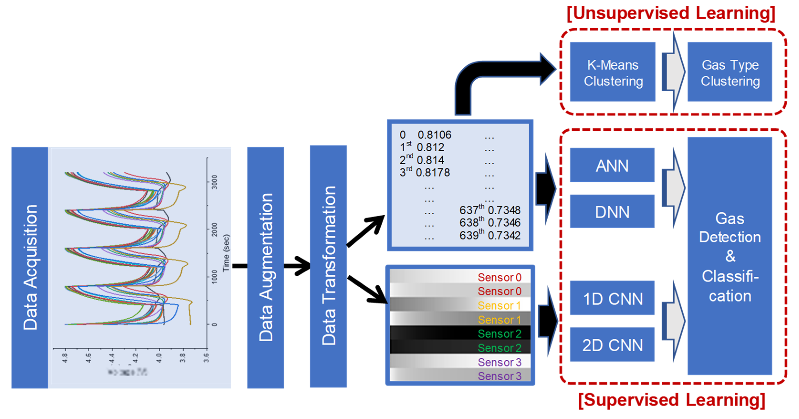
Figure 1. Machine learning approaches for gas classification that incorporate unsupervised learning via K-means clustering and supervised learning algorithms, namely, ANN, DNN, 1D CNN, and 2D CNN.
Electronics 11 03884 g001
Figure 2. Gas sensing responses obtained from four SMO gas sensors ((a) S0 for the NOx sensor; (b) S1 for the VOC sensor; (c) S2 for the CO sensor; (d) S3 for the alcohol sensor), according to artificially designed gas mixture combinations tuned to deep learning-assisted gas detection/classification are described in Table 1. (Note that the total number of gas mixtures is 15).
Electronics 11 03884 g002
Figure 3. (a) Gas sensing data replotted as a function of gas mixture type, i.e., N2, CO, alcohol, and CO/alcohol; (b) example of cluster formation of 4 clusters obtained from a 4-sensor array combination; (c) cluster formation of 4 clusters as a function of sensor combination from 4 single sensors to a single 4-sensor mode; (d) purity information obtained from labeled gas combination sensor data from various sensor combinations using K = 4.
Electronics 11 03884 g003
Figure 4. Architecture of machine learning algorithms employed in gas detection/classification: (a) ANN (2-layer structure), (b) DNN (4-layer structure), (c) 1D CNN, and (d) 2D CNN.
Electronics 11 03884 g004
Figure 5. Accuracy information obtained as a function of the number of sensors and deep learning algorithms employed in gas detection/classification (based on the calculation at 1000 epochs): ANN (2-layer structure), DNN (4-layer structure), 1D CNN, and 2D CNN.
Electronics 11 03884 g005
Figure 6. Loss information evaluated as a function of the number of sensors and deep learning algorithms employed in gas detection/classification (based on the calculation at 1000 epochs): ANN (2-layer structure), DNN (4-layer structure), 1D CNN, and 2D CNN.
Electronics 11 03884 g006
Figure 7. Summarized comparison of neural network–based prediction performances for evaluating the applicability of deep learning algorithms for gas detection/classification in terms of various sensor combinations and machine learning algorithms. (a) loss information at training phases, (b) loss information at validation phases, and (c) loss information at test phases. (The loss evaluations were assessed as a function of the algorithms (ANN, DNN, 1D CNN, and 2D CNN) and the number of sensors, ranging from 4 single sensors to 4-array sensor configurations, with the total of 15 labeled combinations).
Electronics 11 03884 g007
Table 1. Gas combination labels employed to assess the applicability of machine learning to gas sensing classification of CO and C2H5OH gas mixtures with matrix gas N2.
Label
Number
CO
Flow Rate
[sccm]
C2H5OH
Flow Rate
[sccm]
N2
Flow Rate
[sccm]
CO
Concentration
[ppm]
C2H5OH
Concentration
[ppm]
Mixture
Type
000500000N2
(Group I)
150004500200CO
(Group II)
2100004000400CO
(Group II)
3150003500600CO
(Group II)
4200003000800CO
(Group II)
52500025001000CO
(Group II)
6010004000020C2H5OH
(Group III)
7020003000040C2H5OH
(Group III)
8030002000060C2H5OH
(Group III)
9040001000080C2H5OH
(Group III)
100500000100C2H5OH
(Group III)
1150040005002080CO/C2H5OH
(Group IV)
121000300010004060CO/C2H5OH
(Group IV)
131500200015006040CO/C2H5OH
(Group IV)
142000100020008020CO/C2H5OH
(Group IV)
Publisher’s Note: MDPI stays neutral with regard to jurisdictional claims in published maps and institutional affiliations.