
Comprehensive Analysis of Knowledge Graph Embedding Techniques Benchmarked on Link Prediction


Abstract
1. Introduction
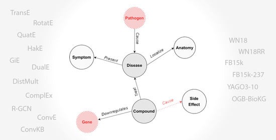
A knowledge graph is a multi-relational graph composed of entities and relations that are regarded as nodes and different types of edges, respectively.
- We compare 13 highly representative encoders belonging to diverse taxonomical families. Following the success of KG representation learning in encoding structural information, such models map entities and relations into a dense space following various strategies, namely translation, semantic matching, and neural network-based.
- We consider six of the most commonly employed datasets taken from four KGs with distinct relational properties.
- We evaluate predictions using a panoply of metrics and criteria, including mean rank, mean reciprocal rank, Hits@n, parameter number, training/evaluation time, and memory consumption.
- Besides considering more quality dimensions, we conduct new experiments for those techniques and datasets not yet covered in the literature, also offering hints in terms of software libraries for practical implementation—an aspect never dealt with by previous works.
- We publicly release all code, datasets, and hyperparameters to ensure maximum reproducibility and foster future research in this area.
2. Literature Survey
3. Materials and Methods
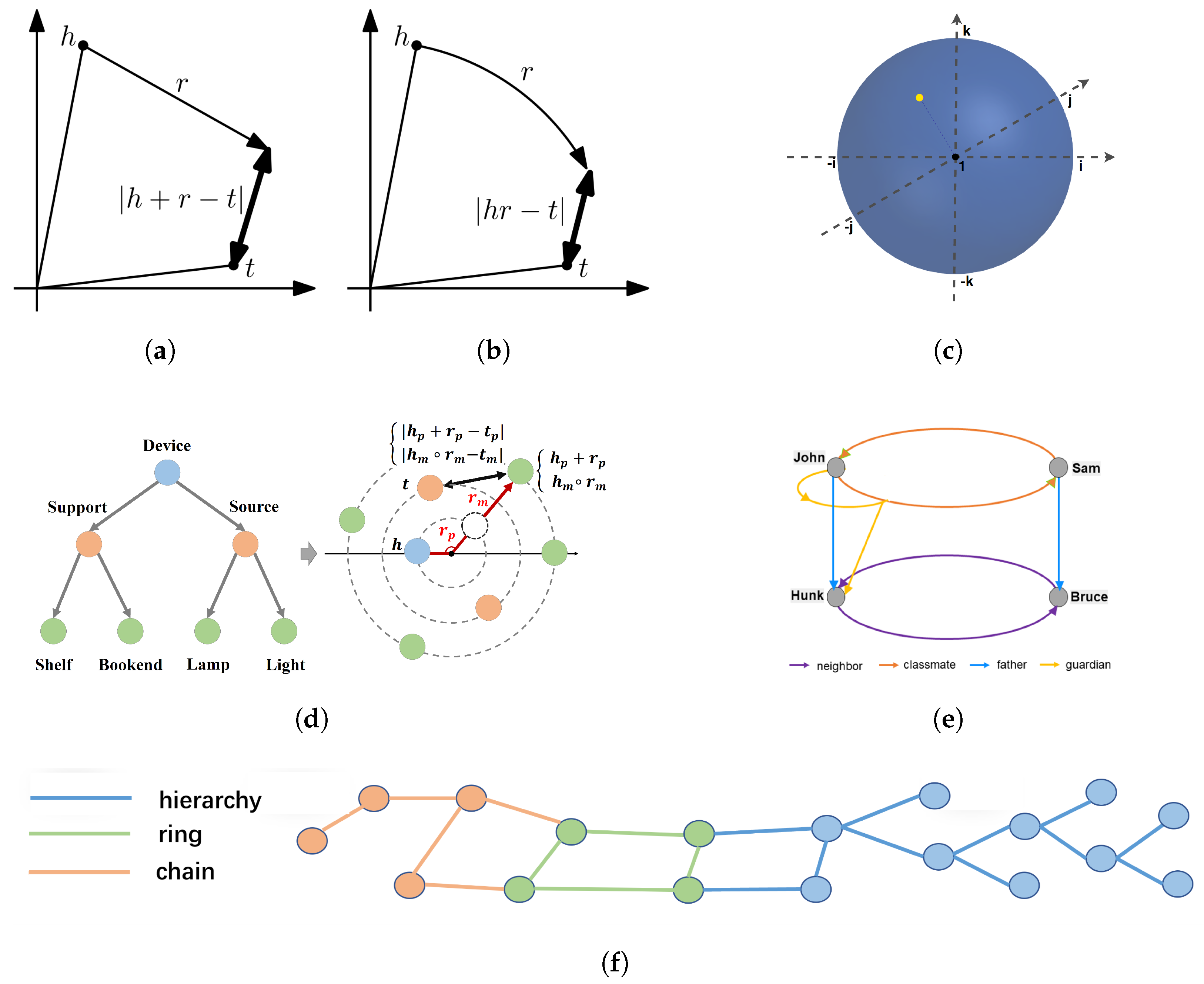
3.1. Relation Patterns
- Symmetry: a relation r is symmetric if ; e.g., “marriage”.
- Antisymmetry: a relation r is antisymmetric if ; e.g., “capital of”.
- Inversion: a relation is inverse to relation if ; e.g.,“has seller” and “is a seller for”.
- Composition: a relation is composed of relation and relation if ; e.g., “my niece is my sister’s daughter”.
3.2. Models
3.2.1. Translation-Based Models
3.2.2. Semantic Matching-Based Models
3.2.3. Based on Neural Networks
3.3. Datasets
3.4. Software Libraries
4. Experimental Setup
4.1. Hardware Settings
4.2. Implementation Details
4.3. Hyperparameters
4.4. Training and Evaluation Protocols
4.5. Evaluation Metrics
5. Results
5.1. Effectiveness
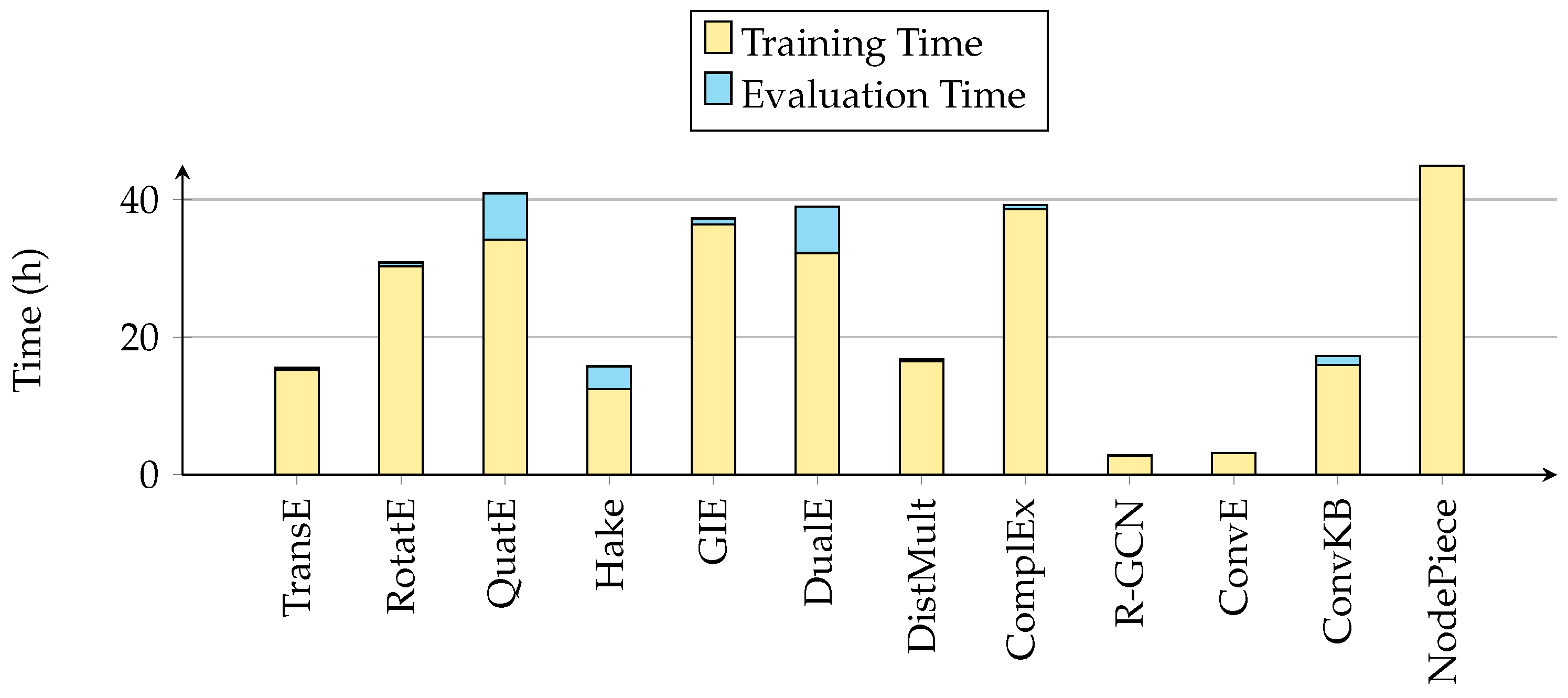
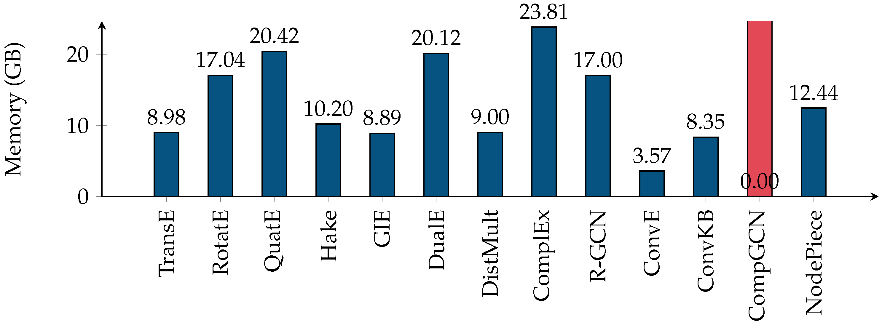
5.2. Efficiency
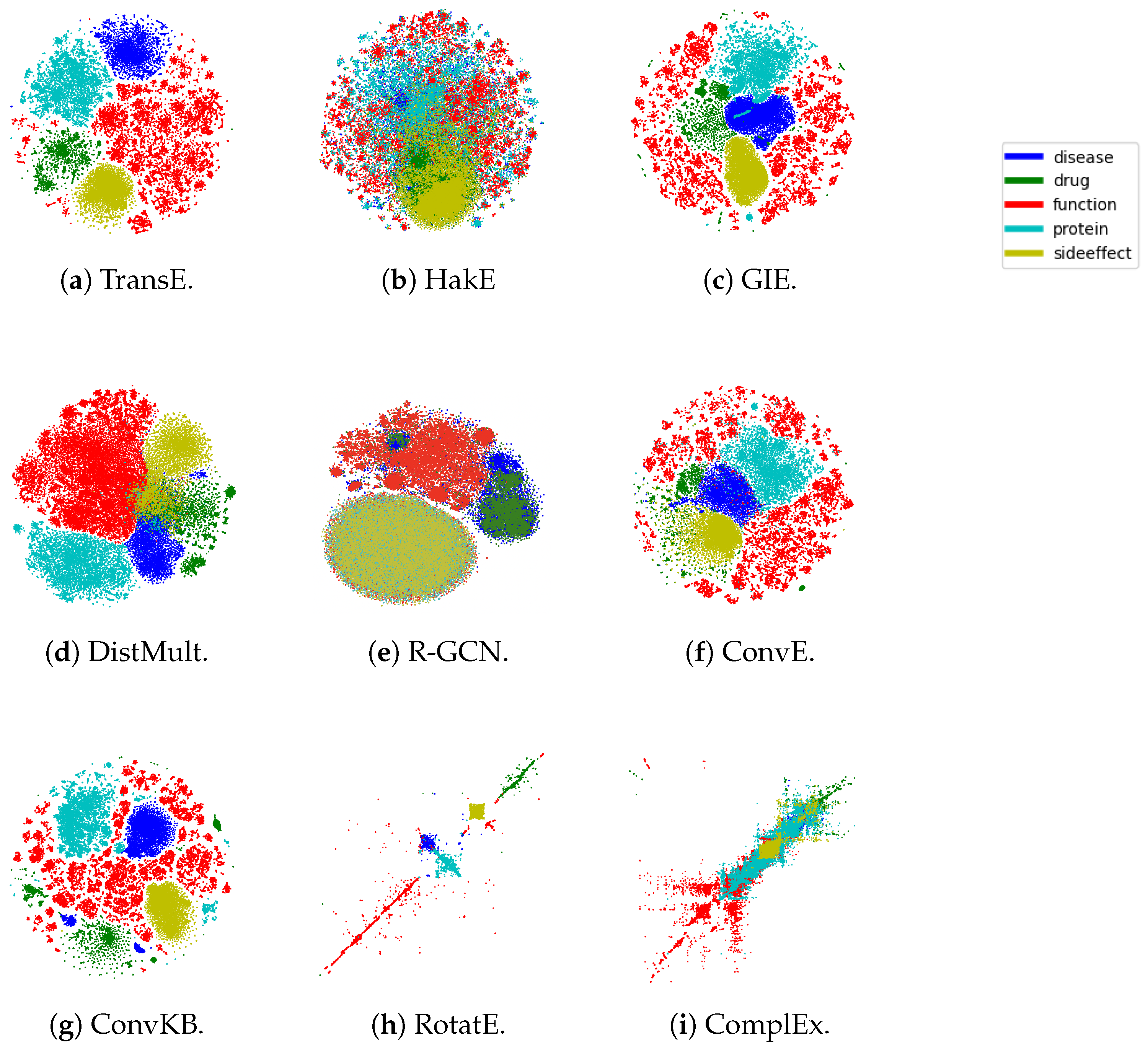
5.3. Embedding Visualization
6. Discussion
7. Conclusions
7.1. Limitations and Future Directions
7.1.1. More Recent Models
7.1.2. Embedding with Auxiliary Information
7.1.3. Data Augmentation
7.1.4. Transfer Learning
7.1.5. Scalability
7.1.6. Dynamic Knowledge
7.1.7. Link Prediction on Semantic Parsing Graphs
Author Contributions
Funding
Institutional Review Board Statement
Informed Consent Statement
Data Availability Statement
Conflicts of Interest
Abbreviations
| GNN | Graph Neural Network |
| GCN | Graph Convolutional Network |
| R-GCN | Relational Graph Convolutional Network |
| KG | Knowledge Graph |
| KGE | Knowledge Graph Embedding |
| LP | Link Prediction |
Appendix A

| Model | Dataset | Hyperparams |
|---|---|---|
| TransE [27] | WN18RR [25] | B:256, Ep:{3000∗, 1000}, D:50, LR:LR:{5 }, :5 |
| FB15K-237 [3] | B: 256, Ep:{3000∗, 1000}, D:{100∗, 50}, LR:{5 ∗, 0.01, 0.1},:1 | |
| YAGO3-10 [5] | B:256, Ep:3000, D:100, LR:{5 ∗, 5 }, :5 | |
| OGB-BIOKG [26] | B:512, Ep:100, D:2000, NSS:128, LR: 5 , :20, AdvTemp:1.0 | |
| RotatE [28] | OGB-BIOKG [26] | B:512, Ep:100, D:2000, NSS:128, LR: 5 , :20, AdvTemp:1.0 |
| QuatE [30] | YAGO3-10 [5] | B:{512∗, 9300}, Ep:1000, D:{100∗, 200}, LR: 0.1, : 1.0, :0.1 |
| OGB-BIOKG [26] | B:512, Ep:100, D:1000, NSS:128, LR: 5 , :20 | |
| HakE [29] | WN18 [25] | B:1024, Steps:180000, D:500, NSS:128, LR:0.0002, :24.0, AdvTemp:1.0, Mod:1.0, Phase:0.5 |
| FB15K [3] | B:1024, Steps:180000, D:500, NSS:128, LR:0.0002, :24.0, AdvTemp:1.0, Mod:1.0, Phase:0.5 | |
| OGB-BIOKG [26] | B:512, Steps:300000, D:2000, NSS:128, LR:0.0002, :24.0, AdvTemp:1.0, Mod:1.0, Phase:0.5 | |
| GIE [32] | WN18 [25] | B:2000, Ep:100, D:2000, LR:0.01, Opt:Adagrad, Reg:N3, RegWeight: 0.1 |
| FB15K [3] | B:2000, Ep:100, D:2000, LR:0.01, Opt:Adagrad, Reg:N3, RegWeight: 0.1 | |
| OGB-BIOKG [26] | B:2000, Ep:100, D:2000, LR:0.01, Opt:Adagrad, Reg:N3, RegWeight: 5 | |
| DualE [31] | YAGO3-10 [5] | B:512, Ep:1000, D:100, LR: 0.1, Opt:adagrad, : 1.0, :0.25 |
| OGB-BIOKG [26] | B:512, Ep:100, D:1000, NSS:128, LR:5 , : 20.0, :0.1 | |
| DistMult [33] | OGB-BIOKG [26] | B:512, Ep:100, D:2000, NSS:128, LR:0.001 :{500∗,1}, AdvTemp:{1.0∗, 0} |
| ComplEx [34] | OGB-BIOKG [26] | B:512, Ep:100, D:2000, NSS:128, LR:0.001, :500, AdvTemp:1.0 |
| R-GCN [37] | FB15K [3] | Ep:50, D:500, LR:0.01, :0.1, Drop:{h:0.2} |
| WN18 [25] | Ep:50, D:500, LR:0.01, :0.1, Drop:{h:0.2} | |
| WN18RR [25] | B:512, Ep:1000, D:150, LR:0.001, :0.0001, Reg:L3, Drop:{h:0.2} | |
| FB15K-237 [3] | Ep:50, D:500, LR:0.01, :0.1, Drop:{h:0.2} | |
| YAGO3-10 [5] | B:512, Ep:1000, D:150, LR:0.001, :0.0001, Reg:L3, Drop:{h:0.2} | |
| OGB-BIOKG [26] | B:65536, Ep:100, D:500, LR:0.001, NSS:1000, Drop:{h:0.2} | |
| ConvE [35] | OGB-BIOKG [26] | B:512, Ep:100, D:2000, NSS:128, LR:0.0001, :20, AdvTemp:1.0, Drop:{in:0.1;h:0.2;feat:0.2} |
| ConvKB [36] | WN18 [25] | B:256, Ep:100, D:50, LR:0.0001, K:64, Drop:{h:0.5} |
| FB15K [3] | B:256, Ep:100, D:50, LR:0.0001, K:{64 ∗, 50}, Drop:{h:{0.5 ∗, 0} | |
| OGB-BIOKG [26] | B:512, Ep:100, D:2000, NSS:128, LR:0.0001, :20, AdvTemp:1.0, K:64, Drop:{h:0.5} | |
| CompGCN [38] | WN18 [25] | B:512, Ep:200, D:200, LR:0.001, :40, N:2, Drop:{h:0.1} |
| FB15K [3] | B:512, Ep:200, D:200, LR:0.001, :40, N:2, Drop:{h:0.1} | |
| YAGO3-10 [5] | B:2048, Ep:100, D:200, LR:0.001, :40, N:2, Drop:{h:0.1} | |
| NodePiece [39] | WN18 [25] | B:512, D: 200, Ep:600, LR:{0.00025∗,0.0005}, NSS: 10, :50, AdvTemp:1.0, Drop:{h:0.1}, :{1000∗,500}, k:{20∗,50}, m:{5∗,4} |
| FB15K [3] | B:512, D: 200, Ep:500, LR:{0.00025∗,0.0005}, NSS: 10, :{50∗,15}, AdvTemp:1.0, Drop:{h:0.1}, :1000, k:20, m:{5∗,15} | |
| OGB-BIOKG [26] | B:512, D: 200, Ep:500, LR:0.0001, NSS: 128, :50, AdvTemp:1.0, Drop:{h:0.1}, :100, k:10, m:6 |
References
- Ji, S.; Pan, S.; Cambria, E.; Marttinen, P.; Philip, S.Y. A survey on knowledge graphs: Representation, acquisition, and applications. IEEE Trans. Neural Netw. Learn. Syst. 2021, 33, 494–514. [Google Scholar] [CrossRef] [PubMed]
- Auer, S.; Bizer, C.; Kobilarov, G.; Lehmann, J.; Cyganiak, R.; Ives, Z. Dbpedia: A nucleus for a web of open data. In The Semantic Web; Springer: Berlin/Heidelberg, Germany, 2007; pp. 722–735. [Google Scholar]
- Bollacker, K.; Evans, C.; Paritosh, P.; Sturge, T.; Taylor, J. Freebase: A collaboratively created graph database for structuring human knowledge. In Proceedings of the 2008 ACM SIGMOD International Conference on Management of Data, Vancouver, BC, Canada, 10–12 June 2008; pp. 1247–1250. [Google Scholar]
- Vrandečić, D.; Krötzsch, M. Wikidata: A Free Collaborative Knowledgebase. Commun. ACM 2014, 57, 78–85. [Google Scholar] [CrossRef]
- Suchanek, F.M.; Kasneci, G.; Weikum, G. Yago: A core of semantic knowledge. In Proceedings of the WWW, Banff, AB, Canada, 8–12 May 2007; ACM: New York, NY, USA, 2007; pp. 697–706. [Google Scholar]
- West, R.; Gabrilovich, E.; Murphy, K.; Sun, S.; Gupta, R.; Lin, D. Knowledge base completion via search-based question answering. In Proceedings of the 23rd International Conference on World Wide Web, Seoul, Republic of Korea, 7–11 April 2014; pp. 515–526. [Google Scholar]
- Krompaß, D.; Baier, S.; Tresp, V. Type-Constrained Representation Learning in Knowledge Graphs. In Proceedings of the ISWC (1); Lecture Notes in Computer Science; Springer: Berlin/Heidelberg, Germany, 2015; Volume 9366, pp. 640–655. [Google Scholar]
- Abbas, K.; Abbasi, A.; Dong, S.; Niu, L.; Yu, L.; Chen, B.; Cai, S.M.; Hasan, Q. Application of network link prediction in drug discovery. BMC Bioinform. 2021, 22, 187. [Google Scholar] [CrossRef]
- Chen, X.; Hu, Z.; Sun, Y. Fuzzy Logic Based Logical Query Answering on Knowledge Graphs. In Proceedings of the AAAI, Virtually, 22 February–1 March 2022; AAAI Press: Palo Alto, CA, USA, 2022; pp. 3939–3948. [Google Scholar]
- Yasunaga, M.; Bosselut, A.; Ren, H.; Zhang, X.; Manning, C.D.; Liang, P.; Leskovec, J. Deep Bidirectional Language-Knowledge Graph Pretraining. In Proceedings of the Neural Information Processing Systems (NeurIPS), New Orleans, LA, USA, 28 November 2022. [Google Scholar]
- Dai, Y.; Wang, S.; Xiong, N.N.; Guo, W. A Survey on Knowledge Graph Embedding: Approaches, Applications and Benchmarks. Electronics 2020, 9, 750. [Google Scholar] [CrossRef]
- Wang, M.; Qiu, L.; Wang, X. A survey on knowledge graph embeddings for link prediction. Symmetry 2021, 13, 485. [Google Scholar] [CrossRef]
- Sharma, A.; Talukdar, P.; Guo, W. Towards understanding the geometry of knowledge graph embeddings. In Proceedings of the 56th Annual Meeting of the Association for Computational Linguistics (Volume 1: Long Papers), Melbourne, Australia, 15–20 July 2018; pp. 122–131. [Google Scholar]
- Akrami, F.; Saeef, M.S.; Zhang, Q.; Hu, W.; Li, C. Realistic re-evaluation of knowledge graph completion methods: An experimental study. In Proceedings of the 2020 ACM SIGMOD International Conference on Management of Data, Portland, OR, USA, 14–19 June 2020; pp. 1995–2010. [Google Scholar]
- Kadlec, R.; Bajgar, O.; Kleindienst, J. Knowledge base completion: Baselines strike back. arXiv 2017, arXiv:1705.10744. [Google Scholar]
- Tran, H.N.; Takasu, A. Analyzing knowledge graph embedding methods from a multi-embedding interaction perspective. arXiv 2019, arXiv:1903.11406. [Google Scholar]
- Wang, Q.; Mao, Z.; Wang, B.; Guo, L. Knowledge graph embedding: A survey of approaches and applications. IEEE Trans. Knowl. Data Eng. 2017, 29, 2724–2743. [Google Scholar] [CrossRef]
- Chen, Z.; Wang, Y.; Zhao, B.; Cheng, J.; Zhao, X.; Duan, Z. Knowledge graph completion: A review. IEEE Access 2020, 8, 192435–192456. [Google Scholar] [CrossRef]
- Choudhary, S.; Luthra, T.; Mittal, A.; Singh, R. A survey of knowledge graph embedding and their applications. arXiv 2021, arXiv:2107.07842. [Google Scholar]
- Garg, S.; Roy, D. A Birds Eye View on Knowledge Graph Embeddings, Software Libraries, Applications and Challenges. arXiv 2022, arXiv:2205.09088. [Google Scholar]
- Hamilton, W.L.; Ying, R.; Leskovec, J. Representation Learning on Graphs: Methods and Applications. IEEE Data Eng. Bull. 2017, 40, 52–74. [Google Scholar]
- Lin, Y.; Han, X.; Xie, R.; Liu, Z.; Sun, M. Knowledge Representation Learning: A Quantitative Review. arXiv 2018, arXiv:1812.10901. [Google Scholar]
- Rossi, A.; Barbosa, D.; Firmani, D.; Matinata, A.; Merialdo, P. Knowledge graph embedding for link prediction: A comparative analysis. ACM Trans. Knowl. Discov. Data (TKDD) 2021, 15, 14. [Google Scholar] [CrossRef]
- Zamini, M.; Reza, H.; Rabiei, M. A Review of Knowledge Graph Completion. Information 2022, 13, 396. [Google Scholar] [CrossRef]
- Miller, G.A. WordNet: A lexical database for English. Commun. ACM 1995, 38, 39–41. [Google Scholar] [CrossRef]
- Hu, W.; Fey, M.; Zitnik, M.; Dong, Y.; Ren, H.; Liu, B.; Catasta, M.; Leskovec, J. Open graph benchmark: Datasets for machine learning on graphs. Adv. Neural Inf. Process. Syst. 2020, 33, 22118–22133. [Google Scholar]
- Bordes, A.; Usunier, N.; Garcia-Duran, A.; Weston, J.; Yakhnenko, O. Translating embeddings for modeling multi-relational data. Adv. Neural Inf. Process. Syst. 2013, 26, 2787–2795. [Google Scholar]
- Sun, Z.; Deng, Z.H.; Nie, J.Y.; Tang, J. Rotate: Knowledge graph embedding by relational rotation in complex space. arXiv 2019, arXiv:1902.10197. [Google Scholar]
- Zhang, Z.; Cai, J.; Zhang, Y.; Wang, J. Learning hierarchy-aware knowledge graph embeddings for link prediction. In Proceedings of the AAAI Conference on Artificial Intelligence, New York, NY, USA, 7–12 February 2020; Volume 34, pp. 3065–3072. [Google Scholar]
- Zhang, S.; Tay, Y.; Yao, L.; Liu, Q. Quaternion knowledge graph embeddings. Adv. Neural Inf. Process. Syst. 2019, 32. [Google Scholar]
- Cao, Z.; Xu, Q.; Yang, Z.; Cao, X.; Huang, Q. Dual quaternion knowledge graph embeddings. In Proceedings of the AAAI Conference on Artificial Intelligence, Virtually, 2–9 February 2021; Volume 35, pp. 6894–6902. [Google Scholar]
- Cao, Z.; Xu, Q.; Yang, Z.; Cao, X.; Huang, Q. Geometry Interaction Knowledge Graph Embeddings. In Proceedings of the AAAI Conference on Artificial Intelligence, Vancouver, BC, Canada, 28 February–1 March 2022. [Google Scholar]
- Yang, B.; Yih, W.T.; He, X.; Gao, J.; Deng, L. Embedding entities and relations for learning and inference in knowledge bases. arXiv 2014, arXiv:1412.6575. [Google Scholar]
- Trouillon, T.; Welbl, J.; Riedel, S.; Gaussier, É.; Bouchard, G. Complex embeddings for simple link prediction. In Proceedings of the International Conference on Machine Learning, PMLR, New York, NY, USA, 20–22 June 2016; pp. 2071–2080. [Google Scholar]
- Dettmers, T.; Minervini, P.; Stenetorp, P.; Riedel, S. Convolutional 2d knowledge graph embeddings. In Proceedings of the AAAI Conference on Artificial Intelligence, New Orleans, LA, USA, 2–7 February 2018; Volume 32. [Google Scholar]
- Nguyen, D.Q.; Nguyen, T.D.; Nguyen, D.Q.; Phung, D. A novel embedding model for knowledge base completion based on convolutional neural network. arXiv 2017, arXiv:1712.02121. [Google Scholar]
- Schlichtkrull, M.; Kipf, T.N.; Bloem, P.; Berg, R.v.d.; Titov, I.; Welling, M. Modeling relational data with graph convolutional networks. In Proceedings of the European Semantic Web Conference, Crete, Greece, 3–7 June 2018; Springer: Berlin/Heidelberg, Germany, 2018; pp. 593–607. [Google Scholar]
- Vashishth, S.; Sanyal, S.; Nitin, V.; Talukdar, P. Composition-based multi-relational graph convolutional networks. arXiv 2019, arXiv:1911.03082. [Google Scholar]
- Galkin, M.; Denis, E.; Wu, J.; Hamilton, W.L. NodePiece: Compositional and Parameter-Efficient Representations of Large Knowledge Graphs. In Proceedings of the International Conference on Learning Representations, Virtually, 25–29 April 2022. [Google Scholar]
- Mikolov, T.; Chen, K.; Corrado, G.; Dean, J. Efficient Estimation of Word Representations in Vector Space. In Proceedings of the ICLR (Workshop Poster), Scottsdale, AZ, USA, 2–4 May 2013. [Google Scholar]
- Wang, Z.; Zhang, J.; Feng, J.; Chen, Z. Knowledge Graph Embedding by Translating on Hyperplanes. In Proceedings of the AAAI, Quebec City, QC, USA, 27–31 July 2014; AAAI Press: Palo Alto, CA, USA, 2014; pp. 1112–1119. [Google Scholar]
- Lin, Y.; Liu, Z.; Sun, M.; Liu, Y.; Zhu, X. Learning Entity and Relation Embeddings for Knowledge Graph Completion. In Proceedings of the AAAI, Austin, TX, USA, 25–30 January 2015; AAAI Press: Palo Alto, CA, USA, 2015; pp. 2181–2187. [Google Scholar]
- Ji, G.; He, S.; Xu, L.; Liu, K.; Zhao, J. Knowledge Graph Embedding via Dynamic Mapping Matrix. In Proceedings of the ACL (1); The Association for Computer Linguistics: New York, NY, USA, 2015; pp. 687–696. [Google Scholar]
- Lodi, S.; Moro, G.; Sartori, C. Distributed data clustering in multi-dimensional peer-to-peer networks. In Proceedings of the Database Technologies 2010, Twenty-First Australasian Database Conference (ADC 2010), Proceedings; CRPIT. Brisbane, Australia, 18–22 January 2010; Shen, H.T., Bouguettaya, A., Eds.; Australian Computer Society: Sydney, Australia, 2010; Volume 104, pp. 171–178. [Google Scholar]
- Cerroni, W.; Moro, G.; Pirini, T.; Ramilli, M. Peer-to-Peer Data Mining Classifiers for Decentralized Detection of Network Attacks. In Proceedings of the Twenty-Fourth Australasian Database Conference, ADC 2013, CRPIT. Adelaide, Australia, 29 January–1 February 2013; Wang, H., Zhang, R., Eds.; Australian Computer Society: Sydney, Australia, 2013; Volume 137, pp. 101–108. [Google Scholar]
- Gilmer, J.; Schoenholz, S.S.; Riley, P.F.; Vinyals, O.; Dahl, G.E. Neural message passing for quantum chemistry. In Proceedings of the International Conference on Machine Learning, PMLR, Sydney, Australia, 6–11 August 2017; pp. 1263–1272. [Google Scholar]
- Han, X.; Cao, S.; Lv, X.; Lin, Y.; Liu, Z.; Sun, M.; Li, J. Openke: An open toolkit for knowledge embedding. In Proceedings of the 2018 Conference on Empirical Methods in Natural Language Processing: System Demonstrations, Brussels, Belgium, 31 October–4 November 2018; pp. 139–144. [Google Scholar]
- Yu, S.Y.; Rokka Chhetri, S.; Canedo, A.; Goyal, P.; Faruque, M.A.A. Pykg2vec: A Python Library for Knowledge Graph Embedding. arXiv 2019, arXiv:1906.04239. [Google Scholar]
- Zhu, Z.; Xu, S.; Tang, J.; Qu, M. Graphvite: A high-performance cpu-gpu hybrid system for node embedding. In Proceedings of the The World Wide Web Conference, San Francisco, CA, USA, 13–17 May 2019; pp. 2494–2504. [Google Scholar]
- Lerer, A.; Wu, L.; Shen, J.; Lacroix, T.; Wehrstedt, L.; Bose, A.; Peysakhovich, A. Pytorch-biggraph: A large scale graph embedding system. Proc. Mach. Learn. Syst. 2019, 1, 120–131. [Google Scholar]
- Zheng, D.; Song, X.; Ma, C.; Tan, Z.; Ye, Z.; Dong, J.; Xiong, H.; Zhang, Z.; Karypis, G. DGL-KE: Training Knowledge Graph Embeddings at Scale. In Proceedings of the 43rd International ACM SIGIR Conference on Research and Development in Information Retrieval (SIGIR ’20), Xi’an, China, 25–30 July 2020; Association for Computing Machinery: New York, NY, USA, 2020; pp. 739–748. [Google Scholar]
- Broscheit, S.; Ruffinelli, D.; Kochsiek, A.; Betz, P.; Gemulla, R. LibKGE—A Knowledge Graph Embedding Library for Reproducible Research. In Proceedings of the 2020 Conference on Empirical Methods in Natural Language Processing: System Demonstrations, Online, 16–20 November 2020; pp. 165–174. [Google Scholar]
- Boschin, A. TorchKGE: Knowledge Graph Embedding in Python and PyTorch. In Proceedings of the International Workshop on Knowledge Graph: Mining Knowledge Graph for Deep Insights, 2020, Virtual Event, 24 August 2020. [Google Scholar]
- Ali, M.; Berrendorf, M.; Hoyt, C.T.; Vermue, L.; Sharifzadeh, S.; Tresp, V.; Lehmann, J. PyKEEN 1.0: A Python Library for Training and Evaluating Knowledge Graph Embeddings. J. Mach. Learn. Res. 2021, 22, 1–6. [Google Scholar]
- Luo, X.; Sun, Z.; Hu, W. μKG: A Library for Multi-source Knowledge Graph Embeddings and Applications. In Proceedings of the ISWC, Hangzhou, China, 23–27 October 2022. [Google Scholar]
- Zhang, W.; Chen, X.; Yao, Z.; Chen, M.; Zhu, Y.; Yu, H.; Huang, Y.; Xu, Y.; Zhang, N.; Xu, Z.; et al. NeuralKG: An Open Source Library for Diverse Representation Learning of Knowledge Graphs. arXiv 2022, arXiv:2202.12571. [Google Scholar]
- Zhang, H.; Yu, Z.; Dai, G.; Huang, G.; Ding, Y.; Xie, Y.; Wang, Y. Understanding gnn computational graph: A coordinated computation, io, and memory perspective. Proc. Mach. Learn. Syst. 2022, 4, 467–484. [Google Scholar]
- Van der Maaten, L.; Hinton, G. Visualizing data using t-SNE. J. Mach. Learn. Res. 2008, 9, 2579–2605. [Google Scholar]
- Zhou, Z.; Wang, C.; Feng, Y.; Chen, D. JointE: Jointly utilizing 1D and 2D convolution for knowledge graph embedding. Knowl.-Based Syst. 2022, 240, 108100. [Google Scholar] [CrossRef]
- Le, T.; Le, N.; Le, B. Knowledge Graph Embedding by Relational Rotation and Complex Convolution for Link Prediction. Expert Syst. Appl. 2022, 214, 119–122. [Google Scholar] [CrossRef]
- Shen, J.; Wang, C.; Gong, L.; Song, D. Joint language semantic and structure embedding for knowledge graph completion. arXiv 2022, arXiv:2209.08721. [Google Scholar]
- Gesese, G.A.; Biswas, R.; Sack, H. A Comprehensive Survey of Knowledge Graph Embeddings with Literals: Techniques and Applications. In Proceedings of the DL4KG@ESWC, CEUR-WS.org, CEUR Workshop, Portoroz, Slovenia, 2 June 2019; Volume 2377, pp. 31–40. [Google Scholar]
- Luo, D.; Cheng, W.; Yu, W.; Zong, B.; Ni, J.; Chen, H.; Zhang, X. Learning to drop: Robust graph neural network via topological denoising. In Proceedings of the 14th ACM International Conference on Web Search and Data Mining, Jerusalem, Israel, 8–12 March 2021; pp. 779–787. [Google Scholar]
- Cai, L.; Ji, S. A multi-scale approach for graph link prediction. In Proceedings of the AAAI Conference on Artificial Intelligence, New York, NY, USA, 7–12 February 2020; Volume 34, pp. 3308–3315. [Google Scholar]
- Wang, J.; Ilievski, F.; Szekely, P.; Yao, K.T. Augmenting Knowledge Graphs for Better Link Prediction. arXiv 2022, arXiv:2203.13965. [Google Scholar]
- Zhao, T.; Liu, G.; Wang, D.; Yu, W.; Jiang, M. Learning from counterfactual links for link prediction. In Proceedings of the International Conference on Machine Learning, PMLR, Baltimore, MD, USA, 17–23 July 2022; pp. 26911–26926. [Google Scholar]
- Wu, X.; Zhang, Y.; Yu, J.; Zhang, C.; Qiao, H.; Wu, Y.; Wang, X.; Wu, Z.; Duan, H. Virtual data augmentation method for reaction prediction. Sci. Rep. 2022, 12, 17098. [Google Scholar] [CrossRef]
- Ding, K.; Xu, Z.; Tong, H.; Liu, H. Data augmentation for deep graph learning: A survey. arXiv 2022, arXiv:2202.08235. [Google Scholar]
- Nayyeri, M.; Cil, G.M.; Vahdati, S.; Osborne, F.; Rahman, M.; Angioni, S.; Salatino, A.; Recupero, D.R.; Vassilyeva, N.; Motta, E.; et al. Trans4E: Link prediction on scholarly knowledge graphs. Neurocomputing 2021, 461, 530–542. [Google Scholar] [CrossRef]
- Baek, J.; Lee, D.B.; Hwang, S.J. Learning to extrapolate knowledge: Transductive few-shot out-of-graph link prediction. Adv. Neural Inf. Process. Syst. 2020, 33, 546–560. [Google Scholar]
- Han, X.; Huang, Z.; An, B.; Bai, J. Adaptive transfer learning on graph neural networks. In Proceedings of the 27th ACM SIGKDD Conference on Knowledge Discovery & Data Mining, Singapore, 14–18 August 2021; pp. 565–574. [Google Scholar]
- Dai, D.; Zheng, H.; Luo, F.; Yang, P.; Chang, B.; Sui, Z. Inductively representing out-of-knowledge-graph entities by optimal estimation under translational assumptions. arXiv 2020, arXiv:2009.12765. [Google Scholar]
- Domeniconi, G.; Moro, G.; Pasolini, R.; Sartori, C. Cross-domain Text Classification through Iterative Refining of Target Categories Representations. In Proceedings of the KDIR 2014–Proceedings of the International Conference on Knowledge Discovery and Information Retrieval, Rome, Italy, 21–24 October 2014; Fred, A.L.N., Filipe, J., Eds.; SciTePress: Setubal, Portugal, 2014; pp. 31–42. [Google Scholar] [CrossRef]
- Domeniconi, G.; Moro, G.; Pagliarani, A.; Pasolini, R. Markov Chain based Method for In-Domain and Cross-Domain Sentiment Classification. In Proceedings of the KDIR 2015—International Conference on Knowledge Discovery and Information Retrieval, Part of the 7th International Joint Conference on Knowledge Discovery, Knowledge Engineering and Knowledge Management (IC3K 2015), Lisbon, Portuga, 12–14 November 2015; Fred, A.L.N., Dietz, J.L.G., Aveiro, D., Liu, K., Filipe, J., Eds.; SciTePress: Setubal, Portugal, 2015; Volume 1, pp. 127–137. [Google Scholar] [CrossRef]
- Domeniconi, G.; Masseroli, M.; Moro, G.; Pinoli, P. Cross-organism learning method to discover new gene functionalities. Comput. Methods Programs Biomed. 2016, 126, 20–34. [Google Scholar] [CrossRef]
- Domeniconi, G.; Moro, G.; Pagliarani, A.; Pasolini, R. On Deep Learning in Cross-Domain Sentiment Classification. In Proceedings of the 9th International Joint Conference on Knowledge Discovery, Knowledge Engineering and Knowledge Management, Funchal, Madeira, Portugal, 1–3 November 2017; Fred, A.L.N., Filipe, J., Eds.; SciTePress: Setubal, Portugal, 2017; Volume 1, pp. 50–60. [Google Scholar] [CrossRef]
- Moro, G.; Pagliarani, A.; Pasolini, R.; Sartori, C. Cross-domain & In-domain Sentiment Analysis with Memory-based Deep Neural Networks. In Proceedings of the IC3K 2018, Seville, Spain, 18–20 September 2018; SciTePress: Setubal, Portugal, 2018; Volume 1, pp. 127–138. [Google Scholar] [CrossRef]
- Frisoni, G.; Moro, G.; Balzani, L. Text-to-Text Extraction and Verbalization of Biomedical Event Graphs. In Proceedings of the 29th International Conference on Computational Linguistics, Gyeongju, Republic of Korea, 12–17 October 2022; International Committee on Computational Linguistics: Gyeongju, Republic of Korea, 2022; pp. 2692–2710. [Google Scholar]
- Nickel, M.; Rosasco, L.; Poggio, T. Holographic embeddings of knowledge graphs. In Proceedings of the AAAI Conference on Artificial Intelligence, Phoenix, AZ, USA, 12–17 February 2016; Volume 30. [Google Scholar]
- Zhang, Y.; Chen, X.; Yang, Y.; Ramamurthy, A.; Li, B.; Qi, Y.; Song, L. Efficient probabilistic logic reasoning with graph neural networks. arXiv 2020, arXiv:2001.11850. [Google Scholar]
- Domeniconi, G.; Masseroli, M.; Moro, G.; Pinoli, P. Discovering New Gene Functionalities from Random Perturbations of Known Gene Ontological Annotations; INSTICC Press: Lisboa, Portugal, 2014; pp. 107–116. [Google Scholar] [CrossRef]
- Fabbri, M.; Moro, G. Dow Jones Trading with Deep Learning: The Unreasonable Effectiveness of Recurrent Neural Networks. In Proceedings of the 7th International Conference on Data Science, Technology and Applications, DATA 2018, Porto, Portugal, 26–28 July 2018; Bernardino, J., Quix, C., Eds.; SciTePress: Setubal, Portugal, 2018; pp. 142–153. [Google Scholar] [CrossRef]
- Cai, B.; Xiang, Y.; Gao, L.; Zhang, H.; Li, Y.; Li, J. Temporal Knowledge Graph Completion: A Survey. arXiv 2022, arXiv:2201.08236. [Google Scholar]
- Moro, G.; Sartori, C. Incremental maintenance of multi-source views. In Proceedings of the Twelfth Australasian Database Conference, ADC2001, Bond University, Queensland, Australia, 29 January–1 February 2001; Orlowska, M.E., Roddick, J.F., Eds.; IEEE Computer Society: Washington, DC, USA, 2001; pp. 13–20. [Google Scholar] [CrossRef]
- Domeniconi, G.; Moro, G.; Pasolini, R.; Sartori, C. Iterative Refining of Category Profiles for Nearest Centroid Cross-Domain Text Classification. In Proceedings of the IC3K 2014, Rome, Italy, 21–24 October 2014; Revised Selected Papers. Springer: Berlin/Heidelberg, Germany, 2014; Volume 553, pp. 50–67. [Google Scholar] [CrossRef]
- Domeniconi, G.; Semertzidis, K.; López, V.; Daly, E.M.; Kotoulas, S.; Moro, G. A Novel Method for Unsupervised and Supervised Conversational Message Thread Detection. In Proceedings of the DATA 2016—5th International Conference on Data Science and Its Applications, Lisbon, Portugal, 24–26 July 2016; SciTePress: Setubal, Portugal, 2016; pp. 43–54. [Google Scholar] [CrossRef]
- Domeniconi, G.; Moro, G.; Pasolini, R.; Sartori, C. A Comparison of Term Weighting Schemes for Text Classification and Sentiment Analysis with a Supervised Variant of tf.idf. In Proceedings of the DATA (Revised Selected Papers); Springer: Berlin/Heidelberg, Germany, 2015; Volume 584, pp. 39–58. [Google Scholar] [CrossRef]
- Moro, G.; Valgimigli, L. Efficient Self-Supervised Metric Information Retrieval: A Bibliography Based Method Applied to COVID Literature. Sensors 2021, 21, 6430. [Google Scholar] [CrossRef]
- Domeniconi, G.; Moro, G.; Pagliarani, A.; Pasini, K.; Pasolini, R. Job Recommendation from Semantic Similarity of LinkedIn Users’ Skills. In Proceedings of the ICPRAM 2016, Rome, Italy, 24–26 February 2016; SciTePress: Setubal, Portugal, 2016; pp. 270–277. [Google Scholar] [CrossRef]
- Frisoni, G.; Moro, G.; Carbonaro, A. Learning Interpretable and Statistically Significant Knowledge from Unlabeled Corpora of Social Text Messages: A Novel Methodology of Descriptive Text Mining. In Proceedings of the DATA 2020—Proc. 9th International Conference on Data Science, Technology and Applications, Online, 7–9 July 2020; SciTePress: Setubal, Portugal, 2020; pp. 121–134. [Google Scholar]
- Frisoni, G.; Moro, G. Phenomena Explanation from Text: Unsupervised Learning of Interpretable and Statistically Significant Knowledge. In Proceedings of the DATA (Revised Selected Papers); Springer: Berlin/Heidelberg, Germany, 2020; Volume 1446, pp. 293–318. [Google Scholar] [CrossRef]
- Frisoni, G.; Moro, G.; Carbonaro, A. Towards Rare Disease Knowledge Graph Learning from Social Posts of Patients. In Proceedings of the RiiForum, Athens, Greece, 15–17 April 2020; Springer: Berlin/Heidelberg, Germany, 2020; pp. 577–589. [Google Scholar] [CrossRef]
- Frisoni, G.; Moro, G.; Carbonaro, A. Unsupervised Descriptive Text Mining for Knowledge Graph Learning. In Proceedings of the IC3K 2020—12th International Joint Conference on Knowledge Discovery, Knowledge Engineering and Knowledge Management, Budapest, Hungary, 2–4 November 2020; SciTePress: Setubal, Portugal, 2020; Volume 1, pp. 316–324. [Google Scholar]
- Banarescu, L.; Bonial, C.; Cai, S.; Georgescu, M.; Griffitt, K.; Hermjakob, U.; Knight, K.; Koehn, P.; Palmer, M.; Schneider, N. Abstract meaning representation for sembanking. In Proceedings of the 7th Linguistic Annotation Workshop and Interoperability with Discourse, Sofia, Bulgaria, 8–9 August 2013; pp. 178–186. [Google Scholar]
- Frisoni, G.; Moro, G.; Carbonaro, A. A Survey on Event Extraction for Natural Language Understanding: Riding the Biomedical Literature Wave. IEEE Access 2021, 9, 160721–160757. [Google Scholar] [CrossRef]
- Oepen, S.; Kuhlmann, M.; Miyao, Y.; Zeman, D.; Cinková, S.; Flickinger, D.; Hajic, J.; Uresova, Z. Semeval 2015 task 18: Broad-coverage semantic dependency parsing. In Proceedings of the 9th International Workshop on Semantic Evaluation (SemEval 2015), Denver, CO, USA, 4–5 June 2015; pp. 915–926. [Google Scholar]
- Abend, O.; Rappoport, A. Universal conceptual cognitive annotation (UCCA). In Proceedings of the 51st Annual Meeting of the Association for Computational Linguistics (Volume 1: Long Papers), Sofia, Bulgaria, 4–9 August 2013; pp. 228–238. [Google Scholar]
- Frisoni, G.; Carbonaro, A.; Moro, G.; Zammarchi, A.; Avagnano, M. NLG-Metricverse: An End-to-End Library for Evaluating Natural Language Generation. In Proceedings of the 29th International Conference on Computational Linguistics, Gyeongju, Republic of Korea, 12–17 October 2022; International Committee on Computational Linguistics: Gyeongju, Republic of Korea, 2022; pp. 3465–3479. [Google Scholar]
- Colon-Hernandez, P.; Havasi, C.; Alonso, J.; Huggins, M.; Breazeal, C. Combining pre-trained language models and structured knowledge. arXiv 2021, arXiv:2101.12294. [Google Scholar]
- Yin, Y.; Meng, F.; Su, J.; Zhou, C.; Yang, Z.; Zhou, J.; Luo, J. A novel graph-based multi-modal fusion encoder for neural machine translation. arXiv 2020, arXiv:2007.08742. [Google Scholar]
- Xu, M.; Li, L.; Wong, D.; Liu, Q.; Chao, L.S. Document graph for neural machine translation. arXiv 2020, arXiv:2012.03477. [Google Scholar]
- Song, L.; Gildea, D.; Zhang, Y.; Wang, Z.; Su, J. Semantic neural machine translation using AMR. Trans. Assoc. Comput. Linguist. 2019, 7, 19–31. [Google Scholar] [CrossRef]
- Huang, L.; Wu, L.; Wang, L. Knowledge Graph-Augmented Abstractive Summarization with Semantic-Driven Cloze Reward. In Proceedings of the 58th Annual Meeting of the Association for Computational Linguistics, ACL 2020, Online, 5–10 July 2020; Jurafsky, D., Chai, J., Schluter, N., Tetreault, J.R., Eds.; Association for Computational Linguistics: Stroudsburg, PA, USA, 2020; pp. 5094–5107. [Google Scholar] [CrossRef]
- Zhu, C.; Hinthorn, W.; Xu, R.; Zeng, Q.; Zeng, M.; Huang, X.; Jiang, M. Enhancing Factual Consistency of Abstractive Summarization. In Proceedings of the 2021 Conference of the North American Chapter of the Association for Computational Linguistics: Human Language Technologies, NAACL-HLT 2021, Online, 6–11 June 2021; Toutanova, K., Rumshisky, A., Zettlemoyer, L., Hakkani-Tür, D., Beltagy, I., Bethard, S., Cotterell, R., Chakraborty, T., Zhou, Y., Eds.; Association for Computational Linguistics: Stroudsburg, PA, USA, 2021; pp. 718–733. [Google Scholar] [CrossRef]
- An, C.; Zhong, M.; Chen, Y.; Wang, D.; Qiu, X.; Huang, X. Enhancing Scientific Papers Summarization with Citation Graph. In Proceedings of the Thirty-Fifth AAAI Conference on Artificial Intelligence, AAAI 2021, Thirty-Third Conference on Innovative Applications of Artificial Intelligence, IAAI 2021, The Eleventh Symposium on Educational Advances in Artificial Intelligence, EAAI 2021, Virtual Event, 2–9 February 2021; AAAI Press: Palo Alto, CA, USA, 2021; pp. 12498–12506. [Google Scholar]
- Ji, X.; Zhao, W. SKGSUM: Abstractive Document Summarization with Semantic Knowledge Graphs. In Proceedings of the International Joint Conference on Neural Networks, IJCNN 2021, Shenzhen, China, 18–22 July 2021; IEEE: Piscataway, NJ, USA, 2021; pp. 1–8. [Google Scholar] [CrossRef]
- Moro, G.; Ragazzi, L. Semantic Self-Segmentation for Abstractive Summarization of Long Legal Documents in Low-Resource Regimes. In Proceedings of the Thirty-Sixth AAAI Conference on Artificial Intelligence, AAAI 2022, Virtual Event, 22 February–1 March 2022; AAAI Press: Palo Alto, CA, USA, 2022; pp. 1–9. [Google Scholar]
- Moro, G.; Ragazzi, L.; Valgimigli, L.; Freddi, D. Discriminative Marginalized Probabilistic Neural Method for Multi-Document Summarization of Medical Literature. In Proceedings of the 60th Annual Meeting of the Association for Computational Linguistics (Volume 1: Long Papers), Dublin, Ireland, 22–27 May 2022; Association for Computational Linguistics: Dublin, Ireland, 2022; pp. 180–189. [Google Scholar] [CrossRef]
- Frisoni, G.; Italiani, P.; Boschi, F.; Moro, G. Enhancing Biomedical Scientific Reviews Summarization with Graph-based Factual Evidence Extracted from Papers. In Proceedings of the 11th International Conference on Data Science, Technology and Applications, DATA 2022, Lisbon, Portugal, 11–13 July 2022; Cuzzocrea, A., Gusikhin, O., van der Aalst, W.M.P., Hammoudi, S., Eds.; SciTePress: Setubal, Portugal, 2022; pp. 168–179. [Google Scholar] [CrossRef]
- Han, J.; Cheng, B.; Wang, X. Open domain question answering based on text enhanced knowledge graph with hyperedge infusion. In Proceedings of the Findings of the Association for Computational Linguistics: EMNLP 2020, Online, 16–20 November 2020; pp. 1475–1481. [Google Scholar]
- Feng, Y.; Chen, X.; Lin, B.Y.; Wang, P.; Yan, J.; Ren, X. Scalable multi-hop relational reasoning for knowledge-aware question answering. arXiv 2020, arXiv:2005.00646. [Google Scholar]
- Yasunaga, M.; Ren, H.; Bosselut, A.; Liang, P.; Leskovec, J. QA-GNN: Reasoning with language models and knowledge graphs for question answering. arXiv 2021, arXiv:2104.06378. [Google Scholar]
- Ying, R.; He, R.; Chen, K.; Eksombatchai, P.; Hamilton, W.L.; Leskovec, J. Graph convolutional neural networks for web-scale recommender systems. In Proceedings of the 24th ACM SIGKDD International Conference on Knowledge Discovery & Data Mining, London, UK, 19–23 August 2018; pp. 974–983. [Google Scholar]
- Guo, Z.; Wang, H. A deep graph neural network-based mechanism for social recommendations. IEEE Trans. Ind. Inform. 2020, 17, 2776–2783. [Google Scholar] [CrossRef]
- Chen, C.; Zhang, M.; Ma, W.; Liu, Y.; Ma, S. Jointly non-sampling learning for knowledge graph enhanced recommendation. In Proceedings of the 43rd International ACM SIGIR Conference on Research and Development in Information Retrieval, Xi’an, China, 25–30 July 2020; pp. 189–198. [Google Scholar]
- Frisoni, G.; Moro, G.; Carlassare, G.; Carbonaro, A. Unsupervised Event Graph Representation and Similarity Learning on Biomedical Literature. Sensors 2022, 22, 3. [Google Scholar] [CrossRef] [PubMed]
- Wu, L.; Chen, Y.; Shen, K.; Guo, X.; Gao, H.; Li, S.; Pei, J.; Long, B. Graph neural networks for natural language processing: A survey. arXiv 2021, arXiv:2106.06090. [Google Scholar]


| Model Families | Datasets | Evaluation | |||||||||||||||
|---|---|---|---|---|---|---|---|---|---|---|---|---|---|---|---|---|---|
| Translation | Semantic Matching | CNN, RNN, Capsule | GNN | WN18 [25] | WN18RR [25] | FB15K [3] | FB15K-237 [3] | YAGO3-10 [5] | OGB-BioKG [26] | LP Metrics | Time Analysis | Memory Analysis | Carbon Footprint | Qualitative Analysis | Unified Dev Framework | Public Code | |
| Lin et al. [23] | ✓(x6) | ✓(x3) | ✓(x1) | ✓ | ✓ | ✓ | ✓ | ✓ | |||||||||
| Rossi et al. [23] | ✓(x5) | ✓(x6) | ✓(x5) | ✓ | ✓ | ✓ | ✓ | ✓ | ✓ | ✓ | ✓ | ||||||
| Wang et al. [12] | ✓(x2) | ✓(x6) | ✓(x2) | ✓(x1) | ✓ | ✓ | ✓ | ✓ | ✓ | ||||||||
| Zamini et al. [24] | ✓(x8) | ✓(x3) | ✓(x8) | ✓(x11) | ✓ | ✓ | ✓ | ||||||||||
| Ours | ✓(x6) | ✓(x2) | ✓(x2) | ✓(x3) | ✓ | ✓ | ✓ | ✓ | ✓ | ✓ | ✓ | ✓ | ✓ | ✓ | ✓ | ✓* | ✓ |
| Model | Entity Embedding | Relation Embedding | Space Complexity |
|---|---|---|---|
| TransE [27] | |||
| RotatE [28] | |||
| QuatE [30] | |||
| HakE [29] | |||
| GIE [32] | - | ||
| DualE [31] | |||
| DistMult [33] | |||
| ComplEx [34] | |||
| R-GCN [37] | |||
| ConvE [35] | |||
| ConvKB [36] | |||
| CompGCN [38] | |||
| NodePiece [39] | - | - | - |
| Triples | Properties | |||||||
|---|---|---|---|---|---|---|---|---|
| Dataset | #Entity | #Relation | #Train | #Valid | #Test | Reified | Test Leakage | Multiple Domains |
| WN18 [25] | 40,943 | 18 | 141,442 | 5000 | 5000 | ✓ | ||
| WN18RR [25] | 40,943 | 11 | 86,835 | 3034 | 3134 | |||
| FB15k [3] | 14,951 | 1345 | 483,142 | 50,000 | 59,071 | ✓ | ✓ | ✓ |
| FB15k-237 [3] | 14,541 | 237 | 272,115 | 17,535 | 20,466 | ✓ | ✓ | |
| YAGO3-10 [5] | 123,182 | 37 | 1,079,040 | 5000 | 5000 | ✓ | ||
| OGB-BioKG [26] | 93,773 | 51 | 4,762,677 | 162,870 | 162,886 | |||
| Library | #Models | #Datasets | HPO | ES | MGPU | DTR | Framework |
|---|---|---|---|---|---|---|---|
| OpenKE [47] | 10 9 | 8 | - | - | - | - | PyTorch TensorFlow |
| Pykg2vec (v0.0.52) [48] | 29 | 10 | ✓ | ✓ | - | - | PyTorch TensorFlow |
| GraphVite (v0.2.2) [49] | 6 | 5 | - | - | ✓ | - | PyTorch |
| PyTorch-BigGraph (v1.0.0) [50] | 4 | 1 | - | - | ✓ | ✓ | PyTorch |
| DGL-KE (v0.1.1) [51] | 6 | 5 | - | - | ✓ | ✓ | PyTorch MXNet |
| LibKGE [52] | 10 | 9 | ✓ | ✓ | - | - | PyTorch |
| TorchKGE (v0.17.5) [53] | 11 | 7 | - | - | - | - | PyTorch |
| PyKEEN (v1.9.0) [54] | 44 | 36 | ✓ | ✓ | * | - | PyTorch PyTorch Lighting |
| muKG [55] | 13 | 14 | - | ✓ | ✓ | ✓ | PyTorch TensorFlow |
| NeuralKG [56] | 19 | 4 | - | - | PyTorch Lighting |
| Datasets | WN18 [25] | FB15K [3] | ||||||||
|---|---|---|---|---|---|---|---|---|---|---|
| Metric | Mean | MRR | Hits@n (%) | Mean | MRR | Hits@n (%) | ||||
| Rank | 1 | 3 | 10 | Rank | 1 | 3 | 10 | |||
| TransE [27] | - | 0.495 | 11.3 | 88.8 | 94.3 | - | 0.463 | 29.7 | 57.8 | 74.9 |
| RotatE [28] | 184 | 0.947 | 93.8 | 95.3 | 96.1 | 32 | 0.699 | 58.5 | 78.8 | 87.2 |
| QuatE [30] | 388 | 0.949 | 94.1 | 95.4 | 96.0 | 41 | 0.770 | 70.0 | 82.1 | 87.8 |
| HakE [29] | 304 | 0.934 | 91.9 | 94.7 | 95.7 | 128 | 0.714 | 63.9 | 76.8 | 83.4 |
| GIE [32] | - | 0.943 | 93.1 | 94.9 | 96.2 | - | 0.805 | 75.2 | 84.1 | 89.4 |
| DualE [31] | 156 | 0.952 | 94.6 | 95.6 | 96.2 | 21 | 0.813 | 76.6 | 85.0 | 89.6 |
| DistMult [33] | 655 | 0.822 | 72.8 | 91.4 | 93.6 | 42 | 0.524 | 54.6 | 73.3 | 82.4 |
| ComplEx [34] | - | 0.941 | 93.6 | 94.5 | 94.7 | - | 0.692 | 59.9 | 75.9 | 84.0 |
| R-GCN [37] | - | 0.819 | 69.7 | 92.9 | 96.4 | - | 0.651 | 54.1 | 73.6 | 82.5 |
| ConvE [35] | 504 | 0.942 | 93.5 | 94.7 | 95.5 | 64 | 0.745 | 67.0 | 80.1 | 87.3 |
| ConvKB [36] | 516 | 0.824 | 74.3 | 89.6 | 94.5 | 109 | 0.567 | 46.2 | 62.9 | 76.2 |
| CompGCN [38] | 539 | 0.676 | 51.8 | 81.6 | 92.1 | 69 | 0.419 | 27.0 | 49.8 | 71.2 |
| NodePiece [39] | 633 | 0.435 | 26.3 | 48.6 | 64.7 | 420 | 0.148 | 7.83 | 15.8 | 28.8 |
| Datasets | WN18RR [25] | FB15K-237 [3] | ||||||||
|---|---|---|---|---|---|---|---|---|---|---|
| Metric | Mean | MRR | Hits@n (%) | Mean | MRR | Hits@n (%) | ||||
| Rank | 1 | 3 | 10 | Rank | 1 | 3 | 10 | |||
| TransE [27] | 2775 | 0.2173 | 3.6 | 36.4 | 49.6 | 334 | 0.218 | 5.52 | 25.7 | 40.7 |
| RotatE [28] | 3277 | 0.476 | 42.8 | 49.2 | 57.1 | 185 | 0.338 | 20.5 | 32.8 | 48.0 |
| QuatE [30] | 3472 | 0.481 | 43.6 | 50.0 | 56.4 | 176 | 0.311 | 22.1 | 34.2 | 49.5 |
| HakE [29] | - | 0.497 | 45.2 | 51.6 | 58.2 | - | 0.346 | 25.0 | 38.1 | 54.2 |
| GIE [32] | - | 0.491 | 45.2 | 50.5 | 57.5 | - | 0.362 | 27.1 | 40.1 | 55.2 |
| DualE [31] | 2270 | 0.492 | 44.4 | 51.3 | 58.4 | 91 | 0.365 | 26.8 | 40.0 | 55.9 |
| DistMult [33] | 5100 | 0.437 | 39 | 44 | 49 | 254 | 0.241 | 15.5 | 26.3 | 41.9 |
| ComplEx [34] | 5261 | 0.436 | 41.0 | 46 | 51 | 339 | 0.247 | 15.8 | 27.5 | 42.8 |
| R-GCN [37] | - | 0.39 | 33.8 | 43.1 | 49 | - | 0.248 | 15.3 | 25.8 | 41.4 |
| ConvE [35] | 5277 | 0.46 | 39.0 | 43.0 | 48.0 | 246 | 0.316 | 23.9 | 35.0 | 49.1 |
| ConvKB [36] | 2554 | 0.248 | - | - | 52.5 | 257 | 0.396 | - | - | 51.7 |
| CompGCN [38] | 3533 | 0.479 | 44.3 | 49.4 | 54.6 | 197 | 0.355 | 26.4 | 39.0 | 53.5 |
| NodePiece [39] | - | 0.403 | - | - | 51.5 | - | 0.256 | - | - | 42.0 |
| Datasets | YAGO3-10 [5] | ||||
|---|---|---|---|---|---|
| Metric | Mean | MRR | Hits@n (%) | ||
| Rank | 1 | 3 | 10 | ||
| TransE [27] | 1156 | 0.118 | 6.7 | 12.8 | 21.2 |
| RotatE [28] | 1767 | 0.495 | 40.2 | 55.0 | 67.0 |
| QuatE [30] | 1281 | 0.260 | 7.5 | 38.5 | 57.6 |
| HakE [29] | - | 0.545 | 46.2 | 59.6 | 69.4 |
| GIE [32] | - | 0.579 | 50.5 | 61.8 | 70.9 |
| DualE [31] | 2068 | 0.280 | 9.6 | 41.6 | 59.1 |
| DistMult [33] | 5926 | 0.340 | 24.0 | 38.0 | 54.0 |
| ComplEx [34] | 6351 | 0.360 | 26.0 | 40.0 | 55.0 |
| R-GCN [37] | - | 0.12 | 6 | 11.3 | 21.1 |
| ConvE [35] | 2792 | 0.520 | 45.0 | 56.0 | 66.0 |
| ConvKB [36] | 2626 | 0.419 | 32.3 | 47.9 | 58.6 |
| CompGCN [38] | 1591 | 0.227 | 12.6 | 25.6 | 44.2 |
| NodePiece [39] | - | 0.247 | - | - | 48.8 |
| Datasets | OGB-BIOKG [26] | ||||
|---|---|---|---|---|---|
| Metric | Mean | MRR | Hits@n (%) | ||
| Rank | 1 | 3 | 10 | ||
| TransE [27] | 222 | 0.154 | 4.9 | 17.7 | 37.1 |
| RotatE [28] | 146 | 0.296 | 13.9 | 37.6 | 60.8 |
| QuatE [30] | 2664 | 0.270 | 21.5 | 29.4 | 37.4 |
| HakE [29] | 333 | 0.290 | 16.2 | 33.8 | 56.4 |
| GIE [32] | - | 0.431 | 31.7 | 48.4 | 65.9 |
| DualE [31] | 502 | 0.336 | 9.1 | 20.5 | 54.5 |
| DistMult [33] | 824 | 0.103 | 2.4 | 11.6 | 26.3 |
| ComplEx [34] | 1964 | 0.219 | 12.8 | 24.8 | 41.2 |
| R-GCN [37] | - | 0.636 | 51.1 | 71.3 | 88.4 |
| ConvE [35] | 444 | 0.276 | 17.2 | 31.8 | 48.9 |
| ConvKB [36] | 476 | 0.206 | 12.5 | 22.3 | 37.1 |
| CompGCN [38] | - | - | - | - | - |
| NodePiece [39] | 201 | 0.230 | 13.4 | 34.3 | 58.7 |
| #params OGBBioKG | TransE [27] | RotatE [28] | QuatE [29] | HakE [30] | GIE [32] | DualE [31] |
|---|---|---|---|---|---|---|
| 187,648,000 | 375,296,000 | 750,242,000 | 375,602,306 | 93,849,502 | 750,242,000 | |
| DistMult [33] | Complex [34] | |||||
| 187,648,000 | 375,296,000 | |||||
| R-GCN [37] | ConvE [35] | ConvKB [36] | CompGCN [38] | NodePiece [39] | ||
| 52,513,000 | 20,943,359 | 187,776,257 | 18,986,250 | 2,761,400 |
| Emissions (g e) | TransE [27] | RotatE [28] | QuatE [29] | HakE [30] | GIE [32] | DualE [31] |
|---|---|---|---|---|---|---|
| 2960 | 5802 | 8216 | 2165 | 6740 | 7472 | |
| DistMult [33] | Complex [34] | |||||
| 3223 | 7384 | |||||
| R-GCN [37] | ConvE [35] | ConvKB [36] | CompGCN [38] | NodePiece [39] | ||
| 505 | 82 | 3943 | - | 9451 |
Publisher’s Note: MDPI stays neutral with regard to jurisdictional claims in published maps and institutional affiliations. |
© 2022 by the authors. Licensee MDPI, Basel, Switzerland. This article is an open access article distributed under the terms and conditions of the Creative Commons Attribution (CC BY) license (https://creativecommons.org/licenses/by/4.0/).
Share and Cite
Ferrari, I.; Frisoni, G.; Italiani, P.; Moro, G.; Sartori, C. Comprehensive Analysis of Knowledge Graph Embedding Techniques Benchmarked on Link Prediction. Electronics 2022, 11, 3866. https://doi.org/10.3390/electronics11233866
Ferrari I, Frisoni G, Italiani P, Moro G, Sartori C. Comprehensive Analysis of Knowledge Graph Embedding Techniques Benchmarked on Link Prediction. Electronics. 2022; 11(23):3866. https://doi.org/10.3390/electronics11233866
Chicago/Turabian StyleFerrari, Ilaria, Giacomo Frisoni, Paolo Italiani, Gianluca Moro, and Claudio Sartori. 2022. "Comprehensive Analysis of Knowledge Graph Embedding Techniques Benchmarked on Link Prediction" Electronics 11, no. 23: 3866. https://doi.org/10.3390/electronics11233866
APA StyleFerrari, I., Frisoni, G., Italiani, P., Moro, G., & Sartori, C. (2022). Comprehensive Analysis of Knowledge Graph Embedding Techniques Benchmarked on Link Prediction. Electronics, 11(23), 3866. https://doi.org/10.3390/electronics11233866