Cost-Sensitive Multigranulation Approximation in Decision-Making Applications

Abstract

A multigranulation rough set (MGRS) model is an expansion of the Pawlak rough set, in which the uncertain concept is characterized by optimistic and pessimistic upper/lower approximate boundaries, respectively. However, there is a lack of approximate descriptions of uncertain concepts by existing information granules in MGRS. The approximation sets of rough sets presented by Zhang provide a way to approximately describe knowledge by using existing information granules. Based on the approximation set theory, this paper proposes the cost-sensitive multigranulation approximation of rough sets, i.e., optimistic approximation and pessimistic approximation. Their related properties were further analyzed. Furthermore, a cost-sensitive selection algorithm to optimize the multigranulation approximation was performed. The experimental results show that when multigranulation approximation sets and upper/lower approximation sets are applied to decision-making environments, multigranulation approximation produces the least misclassification costs on each dataset. In particular, misclassification costs are reduced by more than 50% at each granularity on some datasets.

1. Introduction

As a human-inspired paradigm, granular computing (GrC) solves complex problems by utilizing multiple granular layers [1,2,3,4]. Zadeh [1] noted that information in granules refer to pieces, classes, and groups, into which complex information is divided in accordance with the characteristics and processes of understanding and decision-making. From the different views, GrC models mainly cover four types: fuzzy sets [5], rough sets [6], quotient spaces [7], and cloud models [8]. As representative models of GrC, rough sets describe uncertain concepts by upper and lower approximation boundaries, which have been applied to data mining [9,10], medical systems [11], attribute reductions [12,13], decision systems [14,15], and machine learning [16].

Regarding similarity, Zhang [17,18,19,20] presented the approximation set of rough sets, vague sets, rough fuzzy sets, rough vague sets, etc. These approximation models were developed by utilizing the existing equivalence classes to describe uncertain concepts. The approximation model has a higher similarity with the target concept than the upper/lower approximations. Furthermore, the approximation model has been applied in attribute reduction [21], image segmentation [22], the optimization algorithm [23], etc. Based on the approximation set theory, Yang [24,25] developed the approximation model of rough sets based on misclassification costs. In the process of cost-sensitive learning, the smaller misclassification costs will help to improve the decision-making qualities in real applications. Recently, from the perspective of three-way decisions [26,27,28,29], Yao [30] constructed a symbol–meaning–value (SMV) model for data analysis. In the three-way decision model, the equivalence classes in a boundary region will produce misclassification costs when they are used as approximation sets. Hence, the approximation model that is constructed from the perspective of similarity is no longer applicable to cost-sensitive scenarios. To minimize the misclassification costs of constructing the approximation set, we proposed the multigranulation approximation, i.e., the optimistic approximation model and pessimistic approximation model. Moreover, to search the optimal approximation layer for multigranulation rough sets [31] under the constraints, the algorithm of the cost-sensitive multigranulation approximation selection is further proposed to be applied to decision-making environments.

The following sections are arranged as follows: Section 2 presents the related works. Section 3 introduces the relevant definitions of the multigranulation rough set and approximation set. Section 4 introduces an approximate representation of the rough sets. Section 5 presents the cost-sensitive multigranulation approximations of rough sets and further introduces the optimal multigranulation approximation algorithm. To verify the availability of the proposed model, the related experiments and discussion are presented in Section 6. Ultimately, in Section 7, the conclusions are presented.

2. Literature Review

Rough sets are typically constructed based on a single binary relation. However, in many cases, they may be described in multiple granularity structures. In order to extend single granularity to multi-granularity in rough approximations, Qian [31] proposed the multigranulation rough set model (MGRS), where the upper/lower approximations were defined by multi-equivalence relations (multiple granulations) in the universe [32,33]. For the lower approximation of optimistic MGRS, at least one granular space was obtained, such that objects completely belonged to the target concept. For the lower approximation of pessimistic MGRS, objects completely belong to target concepts in each granular space. MGRS has two advantages: (1) In the process of decision-making applications, the decision of each decision maker may be independent of the same project (or an element) in the universe [34]. In this situation, the intersection operations between any two granularity structures will be redundant for decision-making [35]. (2) Extract decision rules from distributive information systems and groups of intelligent agents by using rough set approaches [34,36].

There are many works [33,34,35,37,38,39,40,41,42] on multigranulation rough sets. To extend the MGRS to the neighborhood information system, Hu [43,44] presented matrix-based incremental approaches to update knowledge about neighborhood information systems by changing the granular structures. From the perspective of uncertainty measure, Sun [39] proposed a feature selection based on fuzzy neighborhood multigranulation rough sets. Xu [38] proposed a dynamic approximation update mechanism of a multigranulation neighborhood rough set from a local viewpoint. Liu [35] introduced a parameter-free multi-granularity attribute reduction scheme, which is more effective for microarray data than other well-established attribute reductions. Based on the three-way decision theory, She [40] presented a five-valued logic approach for the multigranulation rough set model. From the above, however, the method of approximately describing the target concept with existing information granules is not given, which limits the application of the multigranulation rough set theory. Li [41] presented two kinds of local multigranulation rough set models in the ordered decision system by extending the single granulation environment to a multigranulation case. Zhang [42] constructed hesitant fuzzy multigranulation rough sets to handle the hesitant fuzzy information and group decision-making for person–job fit.

3. Preliminaries

In this section, some necessary definitions related to the multigranulation rough set and approximation set are reviewed to facilitate the framework of this paper. Let $S=(U,C\cup D,V,f)$ be a decision information table, where U is a non-empty finite set of objects, C is a non-empty finite set of condition attributes, D is a set of decision attributes, V is the set of all attribute values, and $f:U\times C$ is an information function.

Definition 1 

((Rough Sets) [6]). Let $S=(U,C\cup D,V,f)$ be a decision information table, $A\subseteq C$ and $X\subseteq U$, the lower and upper approximation sets of X are given as follows:

$$\begin{array}{cc}\hfill & \underline{A}\left(X\right)=\{\left.x\in U\right|{\left[x\right]}_A\subseteq X\},\hfill \\ \hfill & \overline{A}\left(X\right)=\{\left.x\in U\right|{\left[x\right]}_A\cap X\ne \varphi \}.\hfill \end{array}$$

where ${\left[x\right]}_A$ denotes the equivalence class induced by $U/\phantom{UA}A$, namely, $U/\phantom{UA}A=\left\{{\left[x\right]}_R\right\}=\{{\left[x\right]}_1,{\left[x\right]}_2,\cdots ,{\left[x\right]}_l\}$.

Based on the lower and upper approximations, the universe U can be divided into three disjoint regions, which are expressed as follows:

$$\begin{array}{cc}\hfill & PO{S}_A\left(X\right)=\underline{A}\left(X\right),\hfill \\ \hfill & BN{D}_A\left(X\right)=\overline{A}\left(X\right)-\underline{A}\left(X\right),\hfill \\ \hfill & NE{G}_A\left(X\right)=U-\overline{A}\left(X\right).\hfill \end{array}$$

Definition 2 

((Optimistic multigranulation rough sets) [36]). Let $S=(U,C\cup D,V,f)$ be a decision information table, $A_1,A_2,\dots ,A_m\subseteq C$ and $X\subseteq U$, then the lower and upper approximation sets of X related to $A_1,A_2,\dots ,A_m$ are given as follows:

$$\begin{array}{cc}\hfill & \underline{\sum _{i=1}^m{A}_i^O}\left(X\right)=\{\left.x\right|{\left[x\right]}_{A_1}\subseteq X\vee {\left[x\right]}_{A_2}\subseteq X\vee \dots \vee {\left[x\right]}_{A_m}\subseteq X,x\in U\},\hfill \end{array}$$

(1)

$$\begin{array}{cc}\hfill & \overline{\sum _{i=1}^m{A}_i^O}\left(X\right)=\sim \underline{\sum _{i=1}^m{A}_i^O}(\sim X).\hfill \end{array}$$

(2)

Then, $(\underline{{\displaystyle \sum _{i=1}^m}{A}_i^O}\left(X\right),\overline{{\displaystyle \sum _{i=1}^m}{A}_i^O}\left(X\right))$ is called optimistic multigranulation rough sets. The lower and upper approximation sets of X in optimistic multigranulation rough sets are presented by multiple independent approximation spaces. The boundary regions are defined as follows:

$$\begin{array}{cc}\hfill & BN{D}_{{\displaystyle \sum _{i=1}^m}{A}_i}^O\left(X\right)=\overline{{\displaystyle \sum _{i=1}^m}{A}_i^O}\left(X\right)-\underline{{\displaystyle \sum _{i=1}^m}{A}_i^O}\left(X\right).\hfill \end{array}$$

(3)

Definition 3 

((Pessimistic multigranulation rough sets) [36]). Let $S=(U,C\cup D,V,f)$ be a decision information table, $A_1,A_2,\dots ,A_m\subseteq C$, and $X\subseteq U$. The lower and upper approximation sets of X related to $A_1,A_2,\dots ,A_m$ are given as follows:

$$\begin{array}{cc}\hfill & \underline{\sum _{i=1}^m{A}_i^P}\left(X\right)=\{\left.x\right|{\left[x\right]}_{A_1}\subseteq X\wedge {\left[x\right]}_{A_2}\subseteq X\wedge \dots \wedge {\left[x\right]}_{A_m}\subseteq X,x\in U\},\hfill \end{array}$$

(4)

$$\begin{array}{cc}\hfill & \overline{\sum _{i=1}^m{A}_i^P}\left(X\right)=\sim \underline{\sum _{i=1}^m{A}_i^P}(\sim X).\hfill \end{array}$$

(5)

Then, $(\underline{{\displaystyle \sum _{i=1}^m}{A}_i^P}\left(X\right),\overline{{\displaystyle \sum _{i=1}^m}{A}_i^P}\left(X\right))$ is called pessimistic multigranulation rough sets. The lower and upper approximation sets of X in pessimistic multigranulation rough sets are presented by multiple independent approximation spaces. However, the strategy is different from optimistic multigranulation rough sets. The boundary region is defined as follows:

$$\begin{array}{cc}\hfill & BN{D}_{\sum _{i=1}^m{A}_i}^P\left(X\right)=\overline{\sum _{i=1}^m{A}_i^P}\left(X\right)-\underline{\sum _{i=1}^m{A}_i^P}\left(X\right).\hfill \end{array}$$

(6)

Definition 4 

((Approximation of rough sets) [17]). Let $S=(U,C\cup D,V,f)$ be a decision information table, $A\subseteq C$ and $X\subseteq U$. $U/\phantom{UA}A=\{{\left[x\right]}_1,{\left[x\right]}_2,\cdots ,{\left[x\right]}_l\}$ is a granularity layer on U, then the α-approximation of X on $U/\phantom{UR}A$ is defined as follows:

$$\begin{array}{cc}\hfill & A_{\alpha }\left(X\right)=\cup \left\{{\left[x\right]}_i\left|\overline{\mu }\left({\left[x\right]}_i\right)\ge \alpha ,{\left[x\right]}_i\subseteq U\right.\right\}.\hfill \end{array}$$

(7)

where $0\le \alpha \le 1$, $\overline{\mu }\left({\left[x\right]}_i\right)=\frac{\left|{\left[x\right]}_i\cap X\right|}{\left|{\left[x\right]}_i\right|}$ denotes the membership degree of the equivalence class ${\left[x\right]}_i$ belongs to X.

Example 1. 

Let

Table 1. A decision information table.

	${\mathit{A}}_1$	${\mathit{A}}_2$	${\mathit{A}}_3$	X
$x_1$	0	0	0	0
$x_2$	0	0	1	0
$x_3$	0	1	0	0
$x_4$	0	1	1	1
$x_5$	1	0	0	0
$x_6$	1	0	1	1
$x_7$	1	1	0	1
$x_8$	1	1	1	1

be a decision information table, $A_1,A_2,A_3\subseteq C$ and $X\subseteq U$. For the element $x_4$, the equivalence classes ${\left[x_4\right]}_i(i=1,2,3)$ belonging to X in the multigranulation approximation space are as follows:

$$\begin{array}{cc}\hfill & {\left[x_4\right]}_1=\{x_1,x_2,x_3,x_4\};\hfill \\ \hfill & {\left[x_4\right]}_2=\{x_3,x_4,x_7,x_8\};\hfill \\ \hfill & {\left[x_4\right]}_3=\{x_2,x_4,x_6,x_8\}.\hfill \end{array}$$

Accordingly, the membership degrees are computed:

$$\begin{array}{cc}\hfill & \overline{\mu }\left({\left[x_4\right]}_1\right)=\frac{0+0+0+1}{4}=0.25;\hfill \\ \hfill & \overline{\mu }\left({\left[x_4\right]}_2\right)=\frac{0+1+1+1}{4}=0.75;\hfill \\ \hfill & \overline{\mu }\left({\left[x_4\right]}_3\right)=\frac{0+1+1+1}{4}=0.75.\hfill \end{array}$$

If α is set to 0.5, considering the optimistic approximation, element $x_4$ will be classified into the optimistic lower approximation sets of X due to one of its membership degrees being greater than 0.5. However, if considering the pessimistic approximation, element $x_4$ will only be classified into the pessimistic upper approximation sets of X.

Based on the given conditions, we have:

$$\begin{array}{cc}\hfill X& =\frac{0.25+0.25+0.25}{x_1}+\frac{0.25+0.25+0.75}{x_2}+\frac{0.25+0.75+0.05}{x_3}+\frac{0.25+0.75+0.75}{x_4}\hfill \\ \hfill & +\frac{0.75+0.25+0.25}{x_5}+\frac{0.75+0.25+0.75}{x_6}+\frac{0.75+0.75+0.25}{x_7}+\frac{0.75+0.75+0.75}{x_8}.\hfill \end{array}$$

Then, the results of the optimistic approximations are shown as follows:

$$\begin{array}{cc}\hfill & \underline{\sum _{i=1}^m{A}_i^O}\left(X\right)=\{x_2,x_3,x_4,x_5,x_6,x_7,x_8\},\hfill \\ \hfill & \overline{\sum _{i=1}^m{A}_i^O}\left(X\right)=\{x_1,x_2,x_3,x_4,x_5,x_6,x_7,x_8\},\hfill \\ \hfill & BN{D}_{\sum _{i=1}^m{A}_i}^O\left(X\right)=\left\{x_1\right\}.\hfill \end{array}$$

Moreover, the results of the pessimistic approximations, in this case, are changed as follows:

$$\begin{array}{cc}\hfill & \underline{\sum _{i=1}^m{A}_i^P}\left(X\right)=\left\{x_8\right\},\hfill \\ \hfill & \overline{\sum _{i=1}^m{A}_i^P}\left(X\right)=\{x_1,x_2,x_3,x_4,x_5,x_6,x_7,x_8\},\hfill \\ \hfill & BN{D}_{\sum _{i=1}^m{A}_i}^P\left(X\right)=\{x_1,x_2,x_3,x_4,x_5,x_6,x_7\}.\hfill \end{array}$$

4. Cost-Sensitive Approximation Methods of the Rough Sets

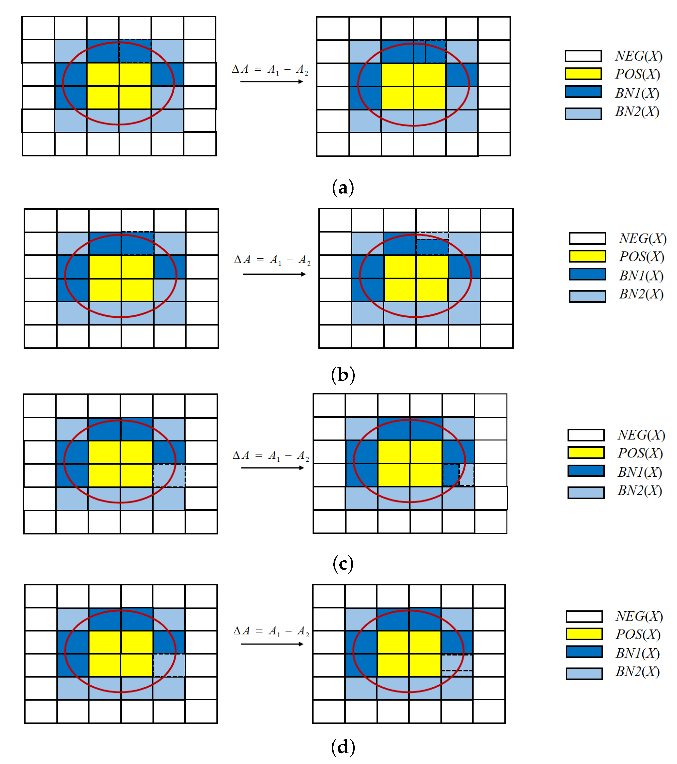
Let $S=(U,C\cup D,V,f)$ be a decision information table, $A\subseteq C$ and $X\subseteq U$. $U/\phantom{UA}A=\{{\left[x\right]}_1,{\left[x\right]}_2,\cdots ,{\left[x\right]}_l\}$ is a granularity layer on U. ${\lambda }_{12}$ represents the cost generated by taking an element belonging to X as the approximation, ${\lambda }_{21}$ represents the cost generated by taking an element that does not belong to X as the approximation. Furthermore, misclassification costs incurred by the equivalence classes in characterizing X on $U/\phantom{UA}A$ are given in the following:

$$\begin{array}{cc}\hfill & {\lambda }^Y={\lambda }_{12}(1-\overline{\mu }\left({\left[x\right]}_i\right))\left|{\left[x\right]}_i\right|.\hfill \end{array}$$

(8)

Misclassification costs incurred by the equivalence classes when not characterizing X on $U/\phantom{UA}A$ are given in the following:

$$\begin{array}{cc}\hfill & {\lambda }^N={\lambda }_{21}\overline{\mu }\left({\left[x\right]}_i\right)\left|{\left[x\right]}_i\right|.\hfill \end{array}$$

(9)

Herein, $\overline{\mu }\left({\left[x\right]}_i\right)(i=1,2,\dots ,l)$ denotes the membership degree of ${\left[x\right]}_i$ belonging to X. Based on the Bayesian decision procedure, the minimum cost decision rules are expressed as follows:

(P)

If ${\lambda }^Y\le {\lambda }^N$, ${\left[x\right]}_i\subseteq A\left(X\right)$;

(N)

If ${\lambda }^Y>{\lambda }^N$, ${\left[x\right]}_i\not\subset A\left(X\right)$.

It is clear that the above rules are only relevant to the loss function $\overline{\mu }\left({\left[x\right]}_i\right)$. From Formulas (8) and (9), the decision rules are re-expressed in the following:

(P1)

If $\overline{\mu }\left({\left[x\right]}_i\right)\ge \frac{{\lambda }_{12}}{{\lambda }_{12}+{\lambda }_{21}}$, ${\left[x\right]}_i\subseteq A\left(X\right)$;

(N1)

If $\overline{\mu }\left({\left[x\right]}_i\right)<\frac{{\lambda }_{12}}{{\lambda }_{12}+{\lambda }_{21}}$, ${\left[x\right]}_i\not\subset A\left(X\right)$.

Supposing $\gamma =\frac{{\lambda }_{12}}{{\lambda }_{12}+{\lambda }_{21}}$, then we have the following decision rules:

(P2)

If $\overline{\mu }\left({\left[x\right]}_i\right)\ge \gamma$, ${\left[x\right]}_i\subseteq A\left(X\right)$;

(N2)

If $\overline{\mu }\left({\left[x\right]}_i\right)<\gamma$, ${\left[x\right]}_i\not\subset A\left(X\right)$.

Definition 5. 

Let $S=(U,C\cup D,V,f)$ be a decision information table, $A\subseteq C$ and $X\subseteq U$. $U/\phantom{UA}A=\{{\left[x\right]}_1,{\left[x\right]}_2,\cdots ,{\left[x\right]}_l\}$ is a granularity layer on U, then the cost-sensitive approximation model (CSA) of rough sets is defined as follows:

$$\begin{array}{cc}\hfill & A\left(X\right)=\cup \left\{{\left[x\right]}_i\left|\overline{\mu }\left({\left[x\right]}_i\right)\ge \frac{{\lambda }_{12}}{{\lambda }_{12}+{\lambda }_{21}},{\left[x\right]}_i\subseteq U\right.\right\}.\hfill \end{array}$$

(10)

Suppose $0\le {\lambda }_{12},{\lambda }_{21}\le 1$, boundary region I and boundary region II are denoted by $BN1\left(X\right)=\{\left.{\left[x\right]}_i\right|\frac{{\lambda }_{12}}{{\lambda }_{12}+{\lambda }_{21}}\le \overline{\mu }\left({\left[x\right]}_i\right)<1\}$ and $BN2\left(X\right)=\{\left.{\left[x\right]}_i\right|0<\overline{\mu }\left({\left[x\right]}_i\right)<\frac{{\lambda }_{12}}{{\lambda }_{12}+{\lambda }_{21}}\}$, respectively, then $BN\left(X\right)=BN1\left(X\right)\cup BN2\left(X\right)$, and $A\left(X\right)=BN1\left(X\right)\cup POS\left(X\right)$. Figure 1 shows the CSA of rough sets, where $BN1\left(X\right)$ is the dark blue region, which denotes the region in the boundary region used as the approximation. $BN2\left(X\right)$ is the light blue region, which denotes the region in the boundary region not used as the approximation. Therefore, the region surrounded by the green broken line in Figure 1 constructs the approximations of rough sets, and the misclassification costs come from two uncertain regions, defined as follows:

$$\begin{array}{cc}\hfill & DC\left(A\left(X\right)\right)=\sum _{{\left[x\right]}_i\in BN1\left(X\right)}{\lambda }^Y+\sum _{{\left[x\right]}_i\in BN2\left(X\right)}{\lambda }^N.\hfill \end{array}$$

(11)

Theorem 1. 

Let $S=(U,A\cup D,V,f)$ be a decision information table, $A_1,A_2,\dots ,$$A_m\subseteq C$, then $DC\left(A_1\left(X\right)\right)\ge DC\left(A_2\left(X\right)\right)$.

Proof of Theorem 1. 

Let U be a non-empty finite domain, ${U/\phantom{UA}A}_1=\{E_1,E_2,\cdots ,E_l\}$ and ${U/\phantom{UA}A}_2=\{F_1,F_2,\cdots ,F_m\}$. Because $A_1\subseteq A_2$, $U/\phantom{U{A}_2}{A}_2\preccurlyeq U/\phantom{U{R}_1}{A}_1$. According to the condition, for simplicity, supposing only one granule $E_1$ can be subdivided into two finer sub-granules by $\mathsf{\Delta }A=A_2-A_1$ (the more complicated cases can be transformed into this case, so we will not repeat them here). Without loss of generality, let $E_1=F_1\cup F_2,E_2=F_3,$$E_3=F_4,\dots ,E_l=F_m$ ($m=l+1$), namely, $U/A_2=\{F_1,F_2,E_2,E_3,\dots ,E_l\}$. There are two cases to prove the theorem as follows:

(1)

Suppose $\overline{\mu }\left(E_1\right)\ge \gamma$, obviously, $E_1\subseteq A_1\left(X\right)$.

Case 1. $\overline{\mu }\left(F_1\right)\ge \gamma$ and $\overline{\mu }\left(F_2\right)\ge \gamma$. Namely, $F_1\subseteq A\left(X\right)$ and $F_2\subseteq A\left(X\right)$. Case 1, in which the granules are subdivided in $BN1\left(X\right)$, can be shown in Figure 2a, then

$$\begin{array}{cc}\hfill \mathsf{\Delta }D{C}_{A_1-A_2}\left(X\right)& =DC\left(A_1\left(X\right)\right)-DC\left(A_2\left(X\right)\right)\hfill \\ \hfill & ={\lambda }_{12}(1-\overline{\mu }\left(E_1\right))\left|E_1\right|-{\lambda }_{12}(1-\overline{\mu }\left(F_1\right))\left|F_1\right|-{\lambda }_{12}(1-\overline{\mu }\left(F_2\right))\left|F_2\right|.\hfill \\ \hfill & =(\left|E_1\right|-\left|F_1\right|-\left|F_2\right|+\sum _{x_i\in F_1}\mu \left(x_i\right)+\sum _{x_i\in F_2}\mu \left(x_i\right)-\sum _{x_i\in E_1}\mu \left(x_i\right)){\lambda }_{12}.\hfill \end{array}$$

Because ${\displaystyle \sum _{x_i\in E_1}}\mu \left(x_i\right)={\displaystyle \sum _{x_i\in F_1}}\mu \left(x_i\right)+{\displaystyle \sum _{x_i\in F_2}}\mu \left(x_i\right)$ and $\left|E_1\right|=\left|F_1\right|+\left|F_2\right|$, then $\mathsf{\Delta }D{C}_{A_1-A_2}=0$. Therefore, $DC\left(A_1\left(X\right)\right)=DC\left(A_2\left(X\right)\right)$.

Case 2. $\overline{\mu }\left(F_1\right)\ge \gamma$ and $\overline{\mu }\left(F_2\right)<\gamma$. Namely, $F_1\subseteq A\left(X\right)$ and $F_2\not\subset A\left(X\right)$. Case 2, in which the granules are subdivided in $BN1\left(X\right)$, can be shown in Figure 2b, then

$$\begin{array}{cc}\hfill \mathsf{\Delta }D{C}_{A_1-A_2}& =DC\left(A_1\left(X\right)\right)-DC\left(A_2\left(X\right)\right)\hfill \\ \hfill & ={\lambda }_{12}(1-\overline{\mu }\left(E_1\right))\left|E_1\right|-{\lambda }_{12}(1-\overline{\mu }\left(F_1\right))\left|F_1\right|-{\lambda }_{21}\overline{\mu }\left(F_2\right)\left|F_2\right|\hfill \\ \hfill & =\left|F_2\right|({\lambda }_{12}-\overline{\mu }\left(F_2\right)({\lambda }_{21}+{\lambda }_{12}))\hfill \end{array}$$

Because $\overline{\mu }\left(F_2\right)<\gamma =\frac{{\lambda }_{12}}{{\lambda }_{12}+{\lambda }_{21}}$ and $\left|E_1\right|=\left|F_1\right|+\left|F_2\right|$, then $\mathsf{\Delta }D{C}_{A_1-A_2}\left(X\right)\ge 0$. Therefore, $DC\left(A_1\left(X\right)\right)>DC\left(A_2\left(X\right)\right)$.

(2)

Suppose $\overline{\mu }\left(E_1\right)<\gamma$, obviously, $E_1\not\subset A_1\left(X\right)$.

Case 1. $\overline{\mu }\left(F_1\right)\ge \gamma$ and $\overline{\mu }\left(F_2\right)<\gamma$. Namely, $F_1\subseteq A\left(X\right)$ and $F_2\not\subset A\left(X\right)$. Case 1, in which the granules are subdivided in $BN2\left(X\right)$, can be shown in Figure 2c, then

$$\begin{array}{cc}\hfill \mathsf{\Delta }D{C}_{A_1-A_2}& =DC\left(A_1\left(X\right)\right)-DC\left(A_2\left(X\right)\right)\hfill \\ \hfill & =\overline{\mu }\left(E_1\right)\left|E_1\right|{\lambda }_{21}-\overline{\mu }\left(F_2\right)\left|F_2\right|{\lambda }_{21}-(1-\overline{\mu }\left(F_1\right))\left|F_1\right|{\lambda }_{12}\hfill \\ \hfill & =\left|F_1\right|\overline{\mu }\left(F_1\right)(({\lambda }_{21}+{\lambda }_{12})-{\lambda }_{12}).\hfill \end{array}$$

Because $\overline{\mu }\left(F_1\right)\ge \gamma =\frac{{\lambda }_{12}}{{\lambda }_{12}+{\lambda }_{21}}$, then $\mathsf{\Delta }D{C}_{A_1-A_2}\ge 0$. Therefore, $DC\left(A_1\left(X\right)\right)\ge DC\left(A_2\left(X\right)\right)$.

Case 2. $\overline{\mu }\left(F_1\right)<\gamma$ and $\overline{\mu }\left(F_2\right)<\gamma$. Namely, $F_1\not\subset R\left(X\right)$ and $F_2\not\subset R\left(X\right)$. Case 2, in which the granules are subdivided in $BN2\left(X\right)$, can be shown in Figure 2d, then

$$\begin{array}{cc}\hfill \mathsf{\Delta }D{C}_{A_1-A_2}& =DC\left(A_1\left(X\right)\right)-DC\left(A_2\left(X\right)\right)\hfill \\ \hfill & =\overline{\mu }\left(E_1\right)\left|E_1\right|{\lambda }_{21}-\overline{\mu }\left(F_1\right)\left|F_1\right|{\lambda }_{21}-\overline{\mu }\left(F_2\right)\left|F_2\right|{\lambda }_{21}\hfill \\ \hfill & =\left(\sum _{x_i\in E_1}\mu \left(x_i\right)-\sum _{x_i\in F_1}\mu \left(x_i\right)-\sum _{x_i\in F_2}\mu \left(x_i\right)\right){\lambda }_{21}.\hfill \end{array}$$

Because ${\displaystyle \sum _{x_i\in E_1}}\mu \left(x_i\right)={\displaystyle \sum _{x_i\in F_1}}\mu \left(x_i\right)+{\displaystyle \sum _{x_i\in F_2}}\mu \left(x_i\right)$, then $\mathsf{\Delta }D{C}_{A_1-A_2}=0$. Therefore, $DC\left(A_1\left(X\right)\right)=DC\left(A_2\left(X\right)\right)$. □

Theorem 1 shows that the misclassification costs in the approximation model will monotonously decrease with the changing approximation space, in accordance with human cognitive mechanisms.

5. Cost-Sensitive Multigranulation Approximations and Optimal Granularity Selection Method

The multigranulation rough set model (MGRS) [43] extends single granularity to multi-granularity in rough approximations to describe an uncertain concept. MGRS is an expansion of the classical rough set, and the target concept is characterized by optimistic and pessimistic upper/lower approximation boundaries in MGRS, respectively. However, there is a lack of an approximate description of an uncertain concept by utilizing the equivalence classes in MGRS. In this section, based on the model proposed in Section 3, we further construct the approximations of MGRS.

5.1. Cost-Sensitive Multigranulation Approximations of Rough Sets

Definition 6. 

Let $S=(U,C\cup D,V,f)$ be a decision information table, $A_1,A_2,\dots ,A_m\subseteq C$ and $X\subseteq U$. The optimistic membership degree of $x\in U$ related to $A_1,A_2,\dots ,A_m$ is given as follows:

$$\begin{array}{cc}\hfill & {\overline{\mu }}_{{\displaystyle \sum _{i=1}^m}{A}_i}^O\left(x\right)=max\left\{\overline{\mu }\left({\left[x\right]}_{A_i}\right)\left|i=1,2,\dots ,m\right.\right\}.\hfill \end{array}$$

(12)

Definition 7. 

Let $S=(U,C\cup D,V,f)$ be a decision information table, $A_1,A_2,\dots ,A_m\subseteq C$ and $X\subseteq U$. The approximation model of the optimistic MGRS of X related to $A_1,A_2,\dots ,A_m$ is given as follows:

$$\begin{array}{cc}\hfill & \sum _{i=1}^m{A}_i^O\left(X\right)=\{\left.x\right|\overline{\mu }\left({\left[x\right]}_{A_1}\right)\ge \gamma \vee \overline{\mu }\left({\left[x\right]}_{A_2}\right)\ge \gamma \vee \dots \vee \overline{\mu }\left({\left[x\right]}_{A_m}\right)\ge \gamma ,x\in U\}.\hfill \end{array}$$

(13)

From the perspective of the optimistic membership degree, ${\displaystyle \sum _{i=1}^m}{A}_i^O\left(X\right)$ can be =expressed as follows:

$$\begin{array}{cc}\hfill & {\displaystyle \sum _{i=1}^m}{A}_i^O\left(X\right)=\{\left.x\right|{\overline{\mu }}_{{\displaystyle \sum _{i=1}^m}{A}_i}^O\left(x\right)\ge \gamma ,x\in U\}.\hfill \end{array}$$

(14)

The corresponding decision regions are defined as follows:

$$\begin{array}{cc}\hfill & BN{1}_{{\displaystyle \sum _{i=1}^m}{A}_i}^O\left(X\right)=\{\left.x\right|1>{\overline{\mu }}_{{\displaystyle \sum _{i=1}^m}{A}_i}^O\left(x\right)\ge \gamma ,x\in U\},\hfill \\ \hfill & BN{2}_{{\displaystyle \sum _{i=1}^m}{A}_i}^O\left(X\right)=\{\left.x\right|0<{\overline{\mu }}_{{\displaystyle \sum _{i=1}^m}{A}_i}^O\left(x\right)<\gamma ,x\in U\},\hfill \\ \hfill & PO{S}_{{\displaystyle \sum _{i=1}^m}{A}_i}^O\left(X\right)=\{\left.x\right|{\overline{\mu }}_{{\displaystyle \sum _{i=1}^m}{A}_i}^O\left(x\right)=1,x\in U\},\hfill \\ \hfill & NE{G}_{{\displaystyle \sum _{i=1}^m}{A}_i}^O\left(X\right)=\{\left.x\right|{\overline{\mu }}_{{\displaystyle \sum _{i=1}^m}{A}_i}^O\left(x\right)=0,x\in U\}.\hfill \end{array}$$

We have

$$\begin{array}{cc}\hfill & {\displaystyle \sum _{i=1}^m}{A}_i^O\left(X\right)=BN{1}_{{\displaystyle \sum _{i=1}^m}{A}_i}^O\left(X\right)\cup PO{S}_{{\displaystyle \sum _{i=1}^m}{A}_i}^O\left(X\right).\hfill \end{array}$$

(15)

The misclassification costs of approximations of optimistic MGRS come from two uncertain regions $BN{1}_{{\displaystyle \sum _{i=1}^m}{A}_i}^O\left(X\right)$ and $BN{2}_{{\displaystyle \sum _{i=1}^m}{A}_i}^O\left(X\right)$, which are defined in the following:

$$\begin{array}{cc}\hfill & DC\left({\displaystyle \sum _{i=1}^m}{A}_i^O\left(X\right)\right)=\sum _{x\in BN{1}_{{\displaystyle \sum _{i=1}^m}{A}_i}^O\left(X\right)}{\lambda }^Y+\sum _{x\in BN{2}_{{\displaystyle \sum _{i=1}^m}{A}_i}^O\left(X\right)}{\lambda }^N.\hfill \end{array}$$

(16)

Theorem 2. 

Let $S=(U,C\cup D,V,f)$ be a decision information table, $A_1,A_2,\dots ,A_m\subseteq C$, $X\subseteq U$ and $X_1,X_2,\dots ,X_n\subseteq U$. The following properties hold:

(1)

${\displaystyle \sum _{i=1}^m}{A}_i^O\left(X\right)={\bigcup }_{i=1}^m{A}_i\left(X\right)$;

(2)

${\displaystyle \sum _{i=1}^m}{A}_i^O\left({\bigcap }_{j=1}^n{X}_j\right)={\bigcup }_{i=1}^m\left({\bigcap }_{j=1}^n{A}_i^O(X_j\right))$;

(3)

${\displaystyle \sum _{i=1}^m}{A}_i^O\left({\bigcap }_{j=1}^n{X}_j\right)\subseteq {\bigcap }_{j=1}^n\left({\displaystyle \sum _{i=1}^m}{A}_i^O\left(X_j\right)\right)$;

(4)

${\displaystyle \sum _{i=1}^m}{A}_i^O\left({\bigcup }_{j=1}^n{X}_j\right)\supseteq {\bigcup }_{j=1}^n\left({\displaystyle \sum _{i=1}^m}{A}_i^O\left(X_j\right)\right)$;

(5)

$\underline{{\displaystyle \sum _{i=1}^m}{A}_i^O}\left(X\right)\subseteq {\displaystyle \sum _{i=1}^m}{A}_i^O\left(X\right)\subseteq \overline{{\displaystyle \sum _{i=1}^m}{A}_i^O}\left(X\right)$.

Proof of Theorem 2. 

(1)

From Formula (14), ${\displaystyle \sum _{i=1}^m}{A}_i^O\left(X\right)={\bigcup }_{i=1}^m{A}_i\left(X\right)$ obviously holds.

(2)

${\displaystyle \sum _{i=1}^m}{A}_i^O\left({\bigcap }_{j=1}^n{X}_j\right)={\bigcup }_{i=1}^m{A}_i^O\left({\bigcap }_{j=1}^n{X}_j\right)={\bigcup }_{i=1}^m\left({\bigcap }_{j=1}^n{A}_i^O(X_j\right))$.

(3)

$\begin{array}{l}{\displaystyle \sum _{i=1}^m}{A}_i^O\left({\bigcap }_{j=1}^n{X}_j\right)={\bigcup }_{i=1}^m\left({\bigcap }_{j=1}^n{A}_i(X_j\right))\\ ={\bigcap }_{j=1}^n({\bigcup }_{i=1}^m{A}_i\left(X_j\right)\cap \cdots \\ ={\bigcap }_{j=1}^n\left({\displaystyle \sum _{i=1}^m}{A}_i^O\left(X_j\right)\right)\cap \cdots \\ ={\bigcap }_{j=1}^n\left({\displaystyle \sum _{i=1}^m}{A}_i^O\left(X_j\right)\right).\end{array}$

(4)

From $X_j\subseteq {\bigcup }_{j=1}^n{X}_j$, we have ${\displaystyle \sum _{i=1}^m}{A}_i^O\left(X_j\right)\subseteq {\displaystyle \sum _{i=1}^m}{A}_i^O\left({\bigcup }_{j=1}^n{X}_j\right)$. Therefore, ${\displaystyle \sum _{i=1}^m}{A}_i^O\left({\bigcup }_{j=1}^n{X}_j\right)\supseteq {\bigcup }_{j=1}^n\left({\displaystyle \sum _{i=1}^m}{A}_i^O\left(X_j\right)\right)$.

(5)

It is easy to prove by Formulas (1), (2), and (14).

 □

Definition 8. 

Let $S=(U,C\cup D,V,f)$ be a decision information table, $A_1,A_2,\dots ,A_m\subseteq C$ and $X\subseteq U$. The pessimistic membership degree of $x\in U$ related to $A_1,A_2,\dots ,A_m$ is given as follows:

$$\begin{array}{cc}\hfill & {\overline{\mu }}_{{\displaystyle \sum _{i=1}^m}{A}_i}^P\left(x\right)=min\left\{\overline{\mu }\left({\left[x\right]}_{A_i}\right)\left|i=1,2,\dots ,m\right.\right\}.\hfill \end{array}$$

(17)

Definition 9. 

Let $S=(U,C\cup D,V,f)$ be a decision information table, $A_1,A_2,\dots ,A_m\subseteq C$ and $X\subseteq U$. The approximation model of pessimistic MGRS of X related to $A_1,A_2,\dots ,A_m$ is given as follows:

$$\begin{array}{cc}\hfill & {\displaystyle \sum _{i=1}^m}{A}_i^P\left(X\right)=\{\left.x\right|\overline{\mu }\left({\left[x\right]}_{A_1}\right)\ge \gamma \wedge \overline{\mu }\left({\left[x\right]}_{A_2}\right)\ge \gamma \wedge \dots \wedge \overline{\mu }\left({\left[x\right]}_{A_m}\right)\ge \gamma ,x\in U\}.\hfill \end{array}$$

(18)

From the perspective of the pessimistic membership degree, ${\displaystyle \sum _{i=1}^m}{A}_i^P\left(X\right)$ can be expressed as follows:

$$\begin{array}{cc}\hfill & {\displaystyle \sum _{i=1}^m}{A}_i^P\left(X\right)=\{\left.x\right|{\overline{\mu }}_{{\displaystyle \sum _{i=1}^m}{A}_i}^P\left(x\right)\ge \gamma ,x\in U\}.\hfill \end{array}$$

(19)

The corresponding decision regions are expressed in the following:

$$\begin{array}{cc}\hfill & BN{1}_{{\displaystyle \sum _{i=1}^m}{A}_i}^P\left(X\right)=\{\left.x\right|1>{\overline{\mu }}_{{\displaystyle \sum _{i=1}^m}{A}_i}^P\left(x\right)\ge \gamma ,x\in U\},\hfill \\ \hfill & BN{2}_{{\displaystyle \sum _{i=1}^m}{A}_i}^P\left(X\right)=\{\left.x\right|0<{\overline{\mu }}_{{\displaystyle \sum _{i=1}^m}{A}_i}^P\left(x\right)<\gamma ,x\in U\},\hfill \\ \hfill & PO{S}_{{\displaystyle \sum _{i=1}^m}{A}_i}^P\left(X\right)=\{\left.x\right|{\overline{\mu }}_{{\displaystyle \sum _{i=1}^m}{A}_i}^P\left(x\right)=1,x\in U\},\hfill \\ \hfill & NE{G}_{{\displaystyle \sum _{i=1}^m}{A}_i}^P\left(X\right)=\{\left.x\right|{\overline{\mu }}_{{\displaystyle \sum _{i=1}^m}{A}_i}^P\left(x\right)=0,x\in U\}.\hfill \end{array}$$

We have

$$\begin{array}{cc}\hfill & {\displaystyle \sum _{i=1}^m}{A}_i^P\left(X\right)=BN{1}_{{\displaystyle \sum _{i=1}^m}{A}_i}^P\left(X\right)\cup PO{S}_{{\displaystyle \sum _{i=1}^m}{A}_i}^P\left(X\right).\hfill \end{array}$$

(20)

The misclassification costs of approximations of optimistic MGRS come from two uncertain regions $BN{1}_{{\displaystyle \sum _{i=1}^m}{A}_i}^P\left(X\right)$ and $BN{2}_{{\displaystyle \sum _{i=1}^m}{A}_i}^P\left(X\right)$, which are defined in the following:

$$\begin{array}{cc}\hfill & DC\left({\displaystyle \sum _{i=1}^m}{A}_i^P\left(X\right)\right)=\sum _{x\in BN{1}_{{\displaystyle \sum _{i=1}^m}{A}_i}^P\left(X\right)}{\lambda }^Y+\sum _{x\in BN{1}_{{\displaystyle \sum _{i=1}^m}{A}_i}^P\left(X\right)}{\lambda }^N.\hfill \end{array}$$

(21)

Theorem 3. 

Let $S=(U,C\cup D,V,f)$ be a decision information table, $A_1,A_2,\dots ,A_m\subseteq C$, $X\subseteq U$ and $X_1,X_2,\dots ,X_n\subseteq U$. The following properties hold:

(1)

${\displaystyle \sum _{i=1}^m}{A}_i^P\left(X\right)={\bigcap }_{i=1}^m\left(A_i\left(X\right)\right);$

(2)

${\displaystyle \sum _{i=1}^m}{A}_i^P\left({\bigcap }_{j=1}^n{X}_j\right)={\bigcap }_{j=1}^n\left({\displaystyle \sum _{i=1}^m}{A}_i^P\left(X_j\right)\right);$

(3)

${\displaystyle \sum _{i=1}^m}{A}_i^P\left({\bigcup }_{j=1}^n{X}_j\right)\supseteq {\bigcup }_{j=1}^n\left({\displaystyle \sum _{i=1}^m}{A}_i^P\left(X_j\right)\right);$

(4)

$\underline{{\displaystyle \sum _{i=1}^m}{A}_i^P}\left(X\right)\subseteq {\displaystyle \sum _{i=1}^m}{A}_i^P\left(X\right)\subseteq \overline{{\displaystyle \sum _{i=1}^m}{A}_i^P}\left(X\right).$

Proof of Theorem 3. 

(1)

$\forall x\in {\displaystyle \sum _{i=1}^m}{A}_i^P\left(X\right)$, according to Definition 9, $\overline{\mu }\left({\left[x\right]}_{A_i}\right)\ge \gamma$ holds, $i=1,2,\cdots ,m$. According to Definition 5, $x\in A_i\left(X\right)$, $i=1,2,\cdots ,m$ and $x\in {\bigcap }_{i=1}^m\left(A_i\left(X\right)\right)$ holds, i.e., ${\displaystyle \sum _{i=1}^m}{A}_i^P\left(X\right)\subseteq {\bigcap }_{i=1}^m\left(A_i\left(X\right)\right)$. $\forall x\in {\bigcap }_{i=1}^m\left(A_i\left(X\right)\right)$, $\overline{\mu }\left({\left[x\right]}_{A_i}\right)\ge \gamma$, $i=1,2,\cdots ,m$. According to Definition 7, $x\in {\displaystyle \sum _{i=1}^m}{A}_i^P\left(X\right)$ holds, i.e., ${\bigcap }_{i=1}^m\left(A_i\left(X\right)\right)\subseteq {\displaystyle \sum _{i=1}^m}{A}_i^P\left(X\right)$. Therefore, we have ${\displaystyle \sum _{i=1}^m}{A}_i^P\left(X\right)={\bigcap }_{i=1}^m\left(A_i\left(X\right)\right)$.

(2)

From the proof of (1), ${\displaystyle \sum _{i=1}^m}{A}_i^P\left({\bigcap }_{j=1}^n{X}_j\right)={\bigcap }_{i=1}^m{A}_i({\bigcap }_{j=1}^n{X}_j)$. According to Definition 7, ${\bigcap }_{i=1}^m{A}_i({\bigcap }_{j=1}^n{X}_j)={\bigcap }_{i=1}^m{\bigcap }_{j=1}^n{A}_i\left(X_j\right)$. Because ${\bigcap }_{i=1}^m{A}_i\left(X_j\right)={\displaystyle \sum _{i=1}^m}{A}_i^P\left(X_j\right)$, ${\displaystyle \sum _{i=1}^m}{A}_i^P\left({\bigcap }_{j=1}^n{X}_j\right)={\bigcap }_{i=1}^m{A}_i({\bigcap }_{j=1}^n{X}_j)={\bigcap }_{j=1}^n{\bigcap }_{i=1}^m{A}_i\left(X_j\right)={\bigcap }_{j=1}^n$$({\displaystyle \sum _{i=1}^m}{A}_i^P\left(X_j\right))$.

(3)

$\forall x\in {\bigcup }_{j=1}^n\left({\displaystyle \sum _{i=1}^m}{A}_i^P\left(X_j\right)\right)$, $\exists X_k(k\in \{1,2,\cdots ,n\})$, $x\in {\displaystyle \sum _{i=1}^m}{A}_i^P\left(X_j\right)$. According to Definition 7, $\forall X_j,j=1,2,\cdots ,n$, $\overline{\mu }\left({\left[x\right]}_{A_i}\right)\ge \gamma$, $,i=1,2,\cdots ,m$, $x\in {\displaystyle \sum _{i=1}^m}{A}_i^P({\bigcup }_{j=1}^n\left(X_j\right))$ holds. Therefore, ${\displaystyle \sum _{i=1}^m}{A}_i^P\left({\bigcup }_{j=1}^n{X}_j\right)\supseteq {\bigcup }_{j=1}^n\left({\displaystyle \sum _{i=1}^m}{A}_i^P\left(X_j\right)\right)$.

(4)

It is easy to prove by Formulas (4), (5), and (19).

 □

Theorem 4. 

Let $S=(U,C\cup D,V,f)$ be a decision information table, $A_1,A_2,\dots ,A_m\subseteq C$ and $X\subseteq U$, $A=A_1\cup A_2\cup \dots \cup A_m$ and $X_1,X_2,\dots ,X_n\subseteq U$. The following properties hold:

(1)

${\displaystyle \sum _{i=1}^m}{A}_i^P\left(X\right)\subseteq {\displaystyle \sum _{i=1}^m}{A}_i^O\left(X\right)\subseteq A\left(X\right);$

(2)

${\displaystyle \sum _{i=1}^{m-1}}{A}_i^O\left(X\right)\subseteq {\displaystyle \sum _{i=1}^m}{A}_i^O\left(X\right)$ and ${\displaystyle \sum _{i=1}^{m-1}}{A}_i^P\left(X\right)\supseteq {\displaystyle \sum _{i=1}^m}{A}_i^P\left(X\right).$

Proof of Theorem 4. 

(1)

According to Definition 6, we only need to prove ${\displaystyle \sum _{i=1}^m}{A}_i^P\left(X\right)\subseteq {\displaystyle \sum _{i=1}^m}{A}_i^O\left(X\right)$. $\forall x\in {\displaystyle \sum _{i=1}^m}{A}_i^P\left(X\right)$, according to Definition 7, $\overline{\mu }\left({\left[x\right]}_{A_i}\right)\ge \gamma$. From Definition 5, we have $x\in {\displaystyle \sum _{i=1}^m}{A}_i^O\left(X\right)$.

(2)

It is easy to prove according to Definitions 5 and 7.

 □

Lemma 1. 

Let $S=(U,C\cup D,V,f)$ be a decision information table, $A\subseteq C$ and $X\subseteq U$, $U/\phantom{UA}A=\{E_1,E_2,...,E_l\}$ is a granularity layer on U. The following properties hold:

(1)

${\displaystyle \sum _{E_i\in BN1\left(X\right)}}{\lambda }_{E_i}^Y\le {\displaystyle \sum _{E_i\in BN1\left(X\right)}}{\lambda }_{E_i}^N;$

(2)

${\displaystyle \sum _{E_i\in BN2\left(X\right)}}{\lambda }_{E_i}^N\le {\displaystyle \sum _{E_i\in BN2\left(X\right)}}{\lambda }_{E_i}^Y.$ Here, $E_i\in U/\phantom{UA}A(i=1,2,\dots ,l)$.

Proof of Lemma 1. 

(1)

${\lambda }_{E_i}^Y-{\lambda }_{E_i}^N={\lambda }_{12}(1-\overline{\mu }\left(E_i\right))\left|E_i\right|-{\lambda }_{21}\overline{\mu }\left(E_i\right)\left|E_i\right|=\left|E_i\right|({\lambda }_{12}-({\lambda }_{12}+{\lambda }_{21}))\overline{\mu }\left(E_i\right)$, because $E_i\in BN1\left(X\right)$, we have $\frac{{\lambda }_{12}}{{\lambda }_{12}+{\lambda }_{21}}\le \overline{\mu }\left(E_i\right)<1$, then ${\lambda }_{E_i}^Y\le {\lambda }_{E_i}^N$, therefore $\sum _{E_i\in BN1\left(X\right)}{\lambda }_{E_i}^Y\le \sum _{E_i\in BN1\left(X\right)}{\lambda }_{E_i}^N$.

(2)

${\lambda }_{E_i}^Y-{\lambda }_{E_i}^N={\lambda }_{12}(1-\overline{\mu }\left(E_i\right))\left|E_i\right|-{\lambda }_{21}\overline{\mu }\left(E_i\right)\left|E_i\right|=\left|E_i\right|({\lambda }_{12}-({\lambda }_{12}+{\lambda }_{21}))\overline{\mu }\left(E_i\right)$. Because $E_i\in BN2\left(X\right)$, we have $0<\overline{\mu }\left(E_i\right)<\frac{{\lambda }_{12}}{{\lambda }_{12}+{\lambda }_{21}}$, then ${\lambda }_{E_i}^Y\ge {\lambda }_{E_i}^N$. Therefore, $\sum _{E_i\in BN2\left(X\right)}{\lambda }_{E_i}^N\le \sum _{E_i\in BN2\left(X\right)}{\lambda }_{E_i}^Y$.

 □

Lemma 1 shows that the misclassification costs incurred by the equivalence classes in characterizing X are not more than the misclassification costs incurred by the equivalence classes when they do not characterize X in $BN1\left(X\right)$. Moreover, misclassification costs incurred by the equivalence classes when they do not characterize X are not more than the misclassification costs incurred by the equivalence classes in characterizing X in $BN2\left(X\right)$.

Theorem 5. 

Let $S=(U,C\cup D,V,f)$ be a decision information table, $A\subseteq C$ and $X\subseteq U$, the following properties hold:

(1)

${\displaystyle \sum _{x\in BN{1}_{{\displaystyle \sum _{i=1}^m}{A}_i}^O\left(X\right)}}{\lambda }_{}^Y\le {\displaystyle \sum _{x\in BN{1}_{{\displaystyle \sum _{i=1}^m}{A}_i}^O\left(X\right)}}{\lambda }_{}^N$ and ${\displaystyle \sum _{x\in BN{1}_{{\displaystyle \sum _{i=1}^m}{A}_i}^P\left(X\right)}}{\lambda }_{}^Y\le {\displaystyle \sum _{x\in BN{1}_{{\displaystyle \sum _{i=1}^m}{A}_i}^P\left(X\right)}}{\lambda }_{}^N;$

(2)

${\displaystyle \sum _{x\in BN{2}_{{\displaystyle \sum _{i=1}^m}{A}_i}^O\left(X\right)}}{\lambda }^N\le {\displaystyle \sum _{x\in BN{2}_{{\displaystyle \sum _{i=1}^m}{A}_i}^O\left(X\right)}}{\lambda }^Y$ and ${\displaystyle \sum _{x\in BN{1}_{{\displaystyle \sum _{i=1}^m}{A}_i}^P\left(X\right)}}{\lambda }^N\le {\displaystyle \sum _{x\in BN{1}_{{\displaystyle \sum _{i=1}^m}{A}_i}^P\left(X\right)}}{\lambda }^Y.$

Proof of Theorem 5. 

From Lemma 1, Theorem 5 holds. □

Theorem 5 shows that misclassification costs incurred by the equivalence classes in characterizing X are not more than misclassification costs incurred by the equivalence classes when they do not characterize X in $BN{1}_{{\displaystyle \sum _{i=1}^m}{A}_i}^O\left(X\right)$ and $BN{1}_{{\displaystyle \sum _{i=1}^m}{R}_i}^P\left(X\right)$. Moreover, misclassification costs incurred by the equivalence classes when they do not characterize X are not more than misclassification costs incurred by the equivalence classes in characterizing X in $BN{2}_{{\displaystyle \sum _{i=1}^m}{A}_i}^O\left(X\right)$ and $BN{2}_{{\displaystyle \sum _{i=1}^m}{A}_i}^P\left(X\right)$.

$DC\left({\displaystyle \sum _{i=1}^m}{A}_i^O\left(X\right)\right)$, $DC\left(\underline{{\displaystyle \sum _{i=1}^m}{A}_i^O}\left(X\right)\right)$ and $DC\left(\overline{{\displaystyle \sum _{i=1}^m}{A}_i^O}\left(X\right)\right)$ denote the misclassification costs generated when ${\displaystyle \sum _{i=1}^m}{A}_i^O\left(X\right)$, $\underline{{\displaystyle \sum _{i=1}^m}{A}_i^O}\left(X\right)$ and $\overline{{\displaystyle \sum _{i=1}^m}{A}_i^O}\left(X\right)$ are approximated to X, respectively. Then, the following theorem holds:

Theorem 6. 

Let $S=(U,C\cup D,V,f)$ be a decision information table, $A\subseteq C$ and $X\subseteq U$, Then, $DC\left({\displaystyle \sum _{i=1}^m}{A}_i^O\left(X\right)\right)\le DC\left(\underline{{\displaystyle \sum _{i=1}^m}{A}_i^O}\left(X\right)\right)$ and $DC\left({\displaystyle \sum _{i=1}^m}{A}_i^O\left(X\right)\right)\le DC\left(\overline{{\displaystyle \sum _{i=1}^m}{A}_i^O}\left(X\right)\right)$.

Proof of Theorem 6. 

When $\underline{{\displaystyle \sum _{i=1}^m}{A}_i^O}\left(X\right)$ is taken as the approximation of X, $DC\left(\underline{{\displaystyle \sum _{i=1}^m}{A}_i^O}\left(X\right)\right)={\displaystyle \sum _{x\in BN\left(X\right)}}{\lambda }^N$; when $\overline{{\displaystyle \sum _{i=1}^m}{A}_i^O}\left(X\right)$ is considered the approximation of X, $DC\left(\overline{{\displaystyle \sum _{i=1}^m}{A}_i^O}\left(X\right)\right)={\displaystyle \sum _{x\in BN\left(X\right)}}{\lambda }^Y$; when $DC\left({\displaystyle \sum _{i=1}^m}{A}_i^O\left(X\right)\right)$ is considered the approximation of X, $DC\left({\displaystyle \sum _{i=1}^m}{A}_i^O\left(X\right)\right)={\displaystyle \sum _{x\in BN1\left(X\right)}}{\lambda }^Y+{\displaystyle \sum _{x\in BN2\left(X\right)}}{\lambda }^N$.

Because $BN\left(X\right)=BN1\left(X\right)\cup BN2\left(X\right)$, we have:

$$\begin{array}{c}\hfill DC\left(\underline{{\displaystyle \sum _{i=1}^m}{A}_i^O}\left(X\right)\right)=\sum _{x\in BN1\left(X\right)}{\lambda }^N+\sum _{x\in BN2\left(X\right)}{\lambda }^N,\\ \hfill DC\left(\overline{{\displaystyle \sum _{i=1}^m}{A}_i^O}\left(X\right)\right)=\sum _{x\in BN1\left(X\right)}{\lambda }^Y+\sum _{x\in BN2\left(X\right)}{\lambda }^Y.\end{array}$$

Therefore, according to Theorem 5,

$$\begin{array}{c}\hfill DC\left({\displaystyle \sum _{i=1}^m}{A}_i^O\left(X\right)\right)\le DC\left(\underline{{\displaystyle \sum _{i=1}^m}{A}_i^O}\left(X\right)\right),\\ \hfill DC\left({\displaystyle \sum _{i=1}^m}{A}_i^O\left(X\right)\right)\le DC\left(\overline{{\displaystyle \sum _{i=1}^m}{A}_i^O}\left(X\right)\right).\end{array}$$

Theorem 6 indicates that when $DC\left({\displaystyle \sum _{i=1}^m}{A}_i^O\left(X\right)\right)$, $DC\left(\underline{{\displaystyle \sum _{i=1}^m}{A}_i^O}\left(X\right)\right)$ and $DC\left(\overline{{\displaystyle \sum _{i=1}^m}{A}_i^O}\left(X\right)\right)$ are used as approximations of X, respectively, $DC\left({\displaystyle \sum _{i=1}^m}{A}_i^O\left(X\right)\right)$ generates the least misclassification costs. □

$DC\left({\displaystyle \sum _{i=1}^m}{A}_i^P\left(X\right)\right)$, $DC\left(\underline{{\displaystyle \sum _{i=1}^m}{A}_i^P}\left(X\right)\right)$ and $DC\left(\overline{{\displaystyle \sum _{i=1}^m}{A}_i^P}\left(X\right)\right)$ denote the misclassification costs generated when ${\displaystyle \sum _{i=1}^m}{A}_i^P\left(X\right)$, $\underline{{\displaystyle \sum _{i=1}^m}{A}_i^P}\left(X\right)$ and $\overline{{\displaystyle \sum _{i=1}^m}{A}_i^P}\left(X\right)$ are approximated to X, respectively.

Theorem 7. 

Let $S=(U,C\cup D,V,f)$ be a decision information table, $A\subseteq C$ and $X\subseteq U$. Then, $DC\left({\displaystyle \sum _{i=1}^m}{A}_i^P\left(X\right)\right)\le DC\left(\underline{{\displaystyle \sum _{i=1}^m}{A}_i^P}\left(X\right)\right)$ and $DC\left({\displaystyle \sum _{i=1}^m}{A}_i^P\left(X\right)\right)\le DC\left(\overline{{\displaystyle \sum _{i=1}^m}{A}_i^P}\left(X\right)\right)$.

Proof of Theorem 7. 

Similar to Theorem 6, Theorem 7 is easy to prove. □

From Theorem 7, when $DC\left({\displaystyle \sum _{i=1}^m}{A}_i^P\left(X\right)\right)$, $DC\left(\underline{{\displaystyle \sum _{i=1}^m}{A}_i^P}\left(X\right)\right)$ and $DC\left(\overline{{\displaystyle \sum _{i=1}^m}{A}_i^P}\left(X\right)\right)$ are used as approximations of X, respectively, $DC\left({\displaystyle \sum _{i=1}^m}{A}_i^P\left(X\right)\right)$ generates the least misclassification costs. Theorems 6 and 7 reflect the advantages of the multigranulation approximation sets that are used for approximating the target concept.

5.2. The Optimal Multigranulation Approximation Selection Method

The objects in the boundary region may be reclassified under different granularities. As a result, the equivalence classes used to represent the approximation set will be changed in the boundary region. In practical applications, the optimal approximation selection should consider both the misclassification and test costs. In MGRS, uncertain concepts characterized in a finer approximation layer result in lower misclassification costs, and test costs increase with the added attributes. Therefore, it is essential to find a balance between misclassification and test costs.

Lemma 2. 

Let $S=(U,C\cup D,V,f)$ be a decision information table, $A_1,A_2,\dots ,A_m\subseteq C$, $A_1\subseteq A_2\subseteq ,\dots ,\subseteq A_m$, and $X\subseteq U$, then $\forall x\in U$, ${\overline{\mu }}_{{\displaystyle \sum _{i=1}^{m-1}}{A}_i}^O\left(x\right)\le {\overline{\mu }}_{{\displaystyle \sum _{i=1}^m}{A}_i}^O\left(x\right)$.

Lemma 3. 

Let $S=(U,C\cup D,V,f)$ be a decision information table, $A_1,A_2,\dots ,A_m\subseteq C$, $A_1\subseteq A_2\subseteq ,\dots ,\subseteq A_m$, and $X\subseteq U$, then $\forall x\in U$, ${\overline{\mu }}_{{\displaystyle \sum _{i=1}^{m-1}}{A}_i}^P\left(x\right)\ge {\overline{\mu }}_{{\displaystyle \sum _{i=1}^m}{A}_i}^P\left(x\right)$.

Theorem 8. 

Let $S=(U,C\cup D,V,f)$ be a decision information table, $A_1,A_2,\dots ,A_m\subseteq C$, $A_1\subseteq A_2\subseteq ,\dots ,\subseteq A_m$ and $X\subseteq U$, only when $\overline{\mu }\left(x\right)$($x\in BN{1}_{{\displaystyle \sum _{i=1}^{m-1}}{A}_i}^O\left(X\right)$) changed with the attribute increased, then $DC\left({\displaystyle \sum _{i=1}^{m-1}}{A}_i^O\left(X\right)\right)\ge DC\left({\displaystyle \sum _{i=1}^m}{A}_i^O\left(X\right)\right)$.

Proof of Theorem 8. 

$$\begin{array}{cc}\hfill DC\left({\displaystyle \sum _{i=1}^m}{A}_i^O\left(X\right)\right)& =\sum _{x\in BN{1}_{{\displaystyle \sum _{i=1}^m}{A}_i}^O\left(X\right)}{\lambda }^Y+\sum _{x\in BN{2}_{{\displaystyle \sum _{i=1}^m}{A}_i}^O\left(X\right)}{\lambda }^N\hfill \\ \hfill & =\sum _{x\in BN{1}_{{\displaystyle \sum _{i=1}^m}{A}_i}^O\left(X\right)}{\lambda }_{12}(1-\overline{\mu }\left(x\right))+\sum _{x\in BN{2}_{{\displaystyle \sum _{i=1}^m}{A}_i}^O\left(X\right)}{\lambda }_{21}\overline{\mu }\left(x\right).\hfill \end{array}$$

According to Lemma 2, we have

$$\begin{array}{cc}\hfill & {\overline{\mu }}_{{\displaystyle \sum _{i=1}^{m-1}}{A}_i}^O\left(x\right)\le {\overline{\mu }}_{{\displaystyle \sum _{i=1}^m}{A}_i}^O\left(x\right).\hfill \end{array}$$

Obviously, $DC\left({\displaystyle \sum _{i=1}^{m-1}}{A}_i^O\left(X\right)\right)\ge DC\left({\displaystyle \sum _{i=1}^m}{A}_i^O\left(X\right)\right)$. □

From Theorem 7, for optimistic MGRS, to reduce the misclassification costs of the approximation, we can add the attribute that only changes the membership of objects in $x\in BN{1}_{{\displaystyle \sum _{i=1}^{m-1}}{A}_i}^O\left(X\right)$.

Theorem 9. 

Let $S=(U,C\cup D,V,f)$ be a decision information table, $A_1,A_2,\dots ,A_m\subseteq C$ and $A_1\subseteq A_2\subseteq ,\dots ,\subseteq A_m$, $X\subseteq U$, only when $\overline{\mu }\left(x\right)$ ($x\in BN{2}_{{\displaystyle \sum _{i=1}^{m-1}}{A}_i}^P\left(X\right)$) changed with the attributes increased, then $DC\left({\displaystyle \sum _{i=1}^{m-1}}{A}_i^P\left(X\right)\right)\ge DC\left({\displaystyle \sum _{i=1}^m}{A}_i^P\left(X\right)\right)$.

Proof of Theorem 9. 

$$\begin{array}{cc}\hfill DC\left({\displaystyle \sum _{i=1}^m}{A}_i^P\left(X\right)\right)& =\sum _{x\in BN{1}_{{\displaystyle \sum _{i=1}^m}{A}_i}^P\left(X\right)}{\lambda }^Y+\sum _{x\in BN{2}_{{\displaystyle \sum _{i=1}^m}{A}_i}^P\left(X\right)}{\lambda }^N\hfill \\ \hfill & =\sum _{x\in BN{1}_{{\displaystyle \sum _{i=1}^m}{A}_i}^P\left(X\right)}{\lambda }_{12}(1-\overline{\mu }\left(x\right))+\sum _{x\in BN{2}_{{\displaystyle \sum _{i=1}^m}{A}_i}^P\left(X\right)}{\lambda }_{21}\overline{\mu }\left(x\right).\hfill \end{array}$$

According to Lemma 3, we have

$$\begin{array}{cc}\hfill & {\overline{\mu }}_{{\displaystyle \sum _{i=1}^{m-1}}{A}_i}^P\left(x\right)\ge {\overline{\mu }}_{{\displaystyle \sum _{i=1}^m}{A}_i}^P\left(x\right).\hfill \end{array}$$

Obviously, $DC\left({\displaystyle \sum _{i=1}^{m-1}}{A}_i^P\left(X\right)\right)\ge DC\left({\displaystyle \sum _{i=1}^m}{A}_i^P\left(X\right)\right)$. □

From Theorem 9, for pessimistic MGRS, to reduce the misclassification costs of the approximation, we can add the attribute that only changes the membership of objects in $x\in BN{2}_{{\displaystyle \sum _{i=1}^{m-1}}{R}_i}^O\left(X\right)$.

In practical applications, on the one hand, the factors included in the test cost, such as money, time, environment, etc., are hard to evaluate objectively. On the other hand, these factors are hard to be integrated because of their different dimensions. In this section, we will evaluate test costs in an attribute-driven form, which are more objective.

Definition 10. 

Let $S=(U,C\cup D,V,f)$ be a decision information table, $a\in C$ and $X\subseteq U$, the significance of a is defined as follows:

$$\begin{array}{cc}\hfill & Sig(a,C,D)=D{C}_{C-\left\{a\right\}}-D{C}_C.\hfill \end{array}$$

(22)

Definition 11. 

Let $S=(U,C\cup D,V,f)$ be a decision information table, $a\in C$, $A\subseteq C$ and $X\subseteq U$; the test cost to construct $A\left(X\right)$ is defined as follows:

$$\begin{array}{cc}\hfill & T{C}_A=\sum _{a\in A}Sig(a,C,D).\hfill \end{array}$$

(23)

In this paper, for simplicity, to present the optimal granularity selection of the multigranulation approximation, we only use the optimistic MGRS as an example.

Definition 12. 

Let $S=(U,C\cup D,V,f)$ be a decision information table, $A_1,A_2,\dots ,A_m\subseteq C$ and $X\subseteq U$; the test cost to construct ${\displaystyle \sum _{i=1}^m}{A}_i^O\left(X\right)$ can be defined as follows:

$$\begin{array}{cc}\hfill & T{C}_{{\displaystyle \sum _{i=1}^m}{A}_i^O}={\displaystyle \sum _{i=1}^m}T{C}_{A_i}.\hfill \end{array}$$

(24)

In this paper, the misclassification and test costs for user requirements are represented as $D{C}_u$ and $T{C}_u$, respectively. A multigranulation approximation ${\displaystyle \sum _{i=1}^k}{A}_i^O\left(X\right)$ is selected to meet the constraints $D{C}_{{\displaystyle \sum _{i=1}^k}{A}_i^O\left(X\right)}\le D{C}_u$ and $T{C}_{{\displaystyle \sum _{i=1}^k}{A}_i^O\left(X\right)}\le T{C}_u$, then the related decision are made on ${\displaystyle \sum _{i=1}^k}{A}_i^O\left(X\right)$. Figure 3 presents the optimal multigranulation approximation selection of optimistic MGRS. Herein, ${\displaystyle \sum _{i=1}^3}{A}_i^O\left(X\right)$ complies with the requirements of the misclassification costs and fails to comply with the requirements of the test costs; $A_1^O\left(X\right)$ complies with the requirements of the test cost and fails to comply with the requirements of misclassification costs; ${\displaystyle \sum _{i=1}^2}{A}_i^O\left(X\right)$ complies with both requirements of misclassification costs and test costs, enabling effective calculations according to granularity optimization. Similarly, the optimal approximation selection of pessimistic MGRS is the same. We formalize the computation as an optimization problem:

$$\underset{k}{argmin}Cos{t}_{{\displaystyle \sum _{i=1}^k}{A}_i^O\left(X\right)},$$

(25)

$$\begin{array}{cc}\hfill s.t.& \\ \hfill & \xi D{C}_{{\displaystyle \sum _{i=1}^k}{A}_i^O\left(X\right)}\le D{C}_u;\hfill \\ \hfill & T{C}_{{\displaystyle \sum _{i=1}^k}{A}_i^O\left(X\right)}\le T{C}_u.\hfill \end{array}$$

where $Cos{t}_{{\displaystyle \sum _{i=1}^k}{A}_i^O\left(X\right)}=\xi D{C}_{{\displaystyle \sum _{i=1}^k}{A}_i^O}+T{C}_{{\displaystyle \sum _{i=1}^k}{A}_i^O}$, and $Cos{t}_{{\displaystyle \sum _{i=1}^k}{A}_i^O\left(X\right)}$ denotes the total cost for constructing ${\displaystyle \sum _{i=1}^k}{A}_i^O\left(X\right)$. $\xi =\frac{\left|U\right|}{\left|{\displaystyle \sum _{i=1}^m}{A}_i^O\left(X\right)\right|}\ast \frac{1}{DC\left(A_m\left(X\right)\right)}$ reflects the contribution degree of the multigranulation approximation layer for the misclassification costs of ${\displaystyle \sum _{i=1}^k}{A}_i^O\left(X\right)$.

5.3. Case Study

Table 2. Evaluation form of the company’s venture capital.

Firm	${\mathit{E}}_1$	${\mathit{E}}_2$	${\mathit{E}}_3$	${\mathit{E}}_4$	${\mathit{E}}_5$	D
$x_1$	3	3	3	3	1	High
$x_2$	2	1	2	3	2	High
$x_3$	2	1	2	1	2	High
·	·	·	·	·	·	·
·	·	·	·	·	·	·
·	·	·	·	·	·	·
$x_{898}$	3	3	2	2	3	Low
$x_{899}$	3	1	3	3	1	Low
$x_{900}$	1	1	3	3	1	Low

is an evaluation form of the company venture capital given by five experts. $U=\{x_1,x_2,\dots ,x_{900}\}$ is 900 investment plans, which are evaluated by 5 experts. The risk level is divided into three categories, including high and low. Suppose that $D{C}_u=5$ and $T{C}_u=2.5$.

(1)

According to the above conditions, the attribute significance can be computed by Formula (25), which is shown in

Table 3. Description of attribute significance.

Attribute	${\mathit{E}}_1$	${\mathit{E}}_2$	${\mathit{E}}_3$	${\mathit{E}}_4$	${\mathit{E}}_5$
$Sig(a,C,D)$	0.74	0.56	0.54	0.36	0.77

.

(2)

Each multigranulation approximation is obtained by adding attributes in ascending order of attribute significance, $E_4\to E_3\to E_2\to E_1\to E_5$ in each stage, respectively. We represent the attributes as follows: $A_1=E_4$, $A_2=E_3$, $A_3=E_2$, $A_4=E_1$, and $A_5=E_5$.

(3)

For each multigranulation approximation layer, $D{C}_{{\displaystyle \sum _{i=1}^k}{A}_i^O}$, $T{C}_{{\displaystyle \sum _{i=1}^k}{A}_i^O}$, and $Cos{t}_{{\displaystyle \sum _{i=1}^k}{A}_i^O\left(X\right)}$ are computed by Formulas (16), (24), and (25), respectively, where $k=1,2,\dots ,5$ and the results are displayed in

Table 4. The description of cost in each multigranulation approximation.

	${\mathit{A}}_1^{\mathit{O}}\left(\mathit{X}\right)$	${\displaystyle \sum _{\mathit{i}=1}^2}{\mathit{A}}_{\mathit{i}}^{\mathit{O}}\left(\mathit{X}\right)$	${\displaystyle \sum _{\mathit{i}=1}^3}{\mathit{A}}_{\mathit{i}}^{\mathit{O}}\left(\mathit{X}\right)$	${\displaystyle \sum _{\mathit{i}=1}^4}{\mathit{A}}_{\mathit{i}}^{\mathit{O}}\left(\mathit{X}\right)$	${\displaystyle \sum _{\mathit{i}=1}^5}{\mathit{A}}_{\mathit{i}}^{\mathit{O}}\left(\mathit{X}\right)$
$\xi DC$	8.3	5.9	4.7	3.6	3.5
$TC$	0.36	0.9	1.46	2.2	2.97
$Cost$	8.66	6.8	6.16	5.8	6.47

.

$Cos{t}_{{\displaystyle \sum _{i=1}^k}{A}_i^O\left(X\right)}$ changes with the increased attributes and only $Cos{t}_{{\displaystyle \sum _{i=1}^3}{A}_i^O\left(X\right)}$ and $Cos{t}_{{\displaystyle \sum _{i=1}^4}{A}_i^O\left(X\right)}$ satisfy $D{C}_{{\displaystyle \sum _{i=1}^k}{A}_i^O\left(X\right)}\le D{C}_u$ and $T{C}_{{\displaystyle \sum _{i=1}^k}{A}_i^O\left(X\right)}\le T{C}_u$ at the same time. According to the Formula (25), we choose the multigranulation approximation layer with the lowest total cost from the above layers; its corresponding approximation layer is ${\displaystyle \sum _{i=1}^3}{A}_i^O\left(X\right)$. Therefore, ${\displaystyle \sum _{i=1}^3}{A}_i^O\left(X\right)$ is the optimal multigranulation approximation used for deciding investment plans, because it possesses lower misclassification costs, i.e., from the perspective of optimistic MGRS, $E_4$, $E_3$, and $E_2$ are reasonable expert sets. The analysis of the case study shows that the proposed method can search for a reasonable approximation under the constraint conditions.

6. Simulation Experiment and Result Analysis

6.1. Simulation Experiment

In this section, the effectiveness and rationality of our model are demonstrated as shown by illustrative experiments. The computer used in the experiments was a WIN 10 operating system with 3.10-GHz CPU and 16.0 GB RAM, and the programming software was MATLAB R2022a. The capability of the proposed model was evaluated on six UCI datasets, which are shown in

Table 5. The description of datasets.

ID	Dataset	Attribute Characteristics	Instances	Condition Attributes
1	Bank	Integer	39	12
2	Breast-Cancer	Integer	699	9
3	Car	Integer	1728	6
4	ENB2012data	Real	768	8
5	Mushroom	Integer	8124	22
6	Tic	Integer	958	9
7	Air Quality	Real	9358	12
8	Concrete	Real	1030	8
9	Hcv	Real	569	10
10	Wisconsin	Real	699	9
11	Zoo	Integer	101	16
12	Balance	Integer	625	4

. In our experiments, we randomly took away some known attribute values from datasets 10–12 to create incomplete decision systems. The missing values are randomly distributed on all conditional attributes.

From Figure 4, for classical rough sets, the misclassification costs of the approximation model monotonously decrease with the granularity being finer, which complies with human cognitive habits.

In Figure 5, $ODC1$, $ODC2$, $ODC3$ and $ODC4$ represent ${\displaystyle \sum _{x\in BN{1}_{{\displaystyle \sum _{i=1}^m}{A}_i}^O\left(X\right)}}{\lambda }^Y$,${\displaystyle \sum _{x\in BN{1}_{{\displaystyle \sum _{i=1}^m}{A}_i}^O\left(X\right)}}{\lambda }^N$, ${\displaystyle \sum _{x\in BN{2}_{{\displaystyle \sum _{i=1}^m}{A}_i}^O\left(X\right)}}{\lambda }^N$ and ${\displaystyle \sum _{x\in BN{2}_{{\displaystyle \sum _{i=1}^m}{A}_i}^O\left(X\right)}}{\lambda }^Y$, respectively. $PDC1$, $PDC2$, $PDC3$ and $PDC4$ represent ${\displaystyle \sum _{x\in BN{1}_{{\displaystyle \sum _{i=1}^m}{A}_i}^P\left(X\right)}}{\lambda }^Y$,${\displaystyle \sum _{x\in BN{1}_{{\displaystyle \sum _{i=1}^m}{A}_i}^P\left(X\right)}}{\lambda }^N$, ${\displaystyle \sum _{x\in BN{2}_{{\displaystyle \sum _{i=1}^m}{A}_i}^P\left(X\right)}}{\lambda }^N$ and ${\displaystyle \sum _{x\in BN{1}_{{\displaystyle \sum _{i=1}^m}{A}_i}^P\left(X\right)}}{\lambda }^Y$, respectively. From Figure 5, under different granular layers, misclassification costs incurred by the equivalence classes in approximating X are always less than or equal to misclassification costs incurred by the equivalence classes when they do not characterize X in $BN{1}_{{\displaystyle \sum _{i=1}^m}{A}_i}^O\left(X\right)$ and $BN{1}_{{\displaystyle \sum _{i=1}^m}{A}_i}^P\left(X\right)$. Moreover, misclassification costs incurred by equivalence classes when they do not characterize X are less than or equal to the misclassification costs incurred by the equivalence classes in approximating X in $BN{2}_{{\displaystyle \sum _{i=1}^m}{A}_i}^O\left(X\right)$ and $BN{2}_{{\displaystyle \sum _{i=1}^m}{A}_i}^P\left(X\right)$. This is consistent with Theorem 4.

In Figure 6, the horizontal and vertical axes denote the granularity and misclassification costs, respectively. $ODC\_lower$, $ODC\_upper$ and $ODC$ represent $DC\left(\underline{{\displaystyle \sum _{i=1}^m}{A}_i^O}\left(X\right)\right)$, $DC\left(\overline{{\displaystyle \sum _{i=1}^m}{A}_i^O}\left(X\right)\right)$ and $DC\left({\displaystyle \sum _{i=1}^m}{A}_i^O\left(X\right)\right)$. $PDC\_lower$, $PDC\_upper$ and $PDC$ represent $DC\left(\underline{{\displaystyle \sum _{i=1}^m}{A}_i^P}\left(X\right)\right)$,$DC\left(\overline{{\displaystyle \sum _{i=1}^m}{A}_i^P}\left(X\right)\right)$ and $DC\left({\displaystyle \sum _{i=1}^m}{A}_i^P\left(X\right)\right)$, respectively, namely, the misclassification costs generated when $\underline{{\displaystyle \sum _{i=1}^m}{A}_i^O}\left(X\right)$, $\overline{{\displaystyle \sum _{i=1}^m}{R}_i^O}\left(X\right)$ and ${\displaystyle \sum _{i=1}^m}{A}_i^O\left(X\right)$ are approximated to X and the misclassification costs generated when $\underline{{\displaystyle \sum _{i=1}^m}{A}_i^P}\left(X\right)$, $\overline{{\displaystyle \sum _{i=1}^m}{A}_i^P}\left(X\right)$ and ${\displaystyle \sum _{i=1}^m}{A}_i^P\left(X\right)$ are approximated to X. Obviously, compared with $\underline{{\displaystyle \sum _{i=1}^m}{A}_i^O}\left(X\right)$ and $\overline{{\displaystyle \sum _{i=1}^m}{A}_i^O}\left(X\right)$, the misclassification costs of ${\displaystyle \sum _{i=1}^m}{A}_i^O\left(X\right)$ are the least on each granularity. Similarly, compared with $\underline{{\displaystyle \sum _{i=1}^m}{A}_i^P}\left(X\right)$,$\overline{{\displaystyle \sum _{i=1}^m}{A}_i^P}\left(X\right)$, the misclassification costs of ${\displaystyle \sum _{i=1}^m}{A}_i^P\left(X\right)$ are the least on each granularity. This is consistent with Theorems 5 and 6.

6.2. Results and Discussions

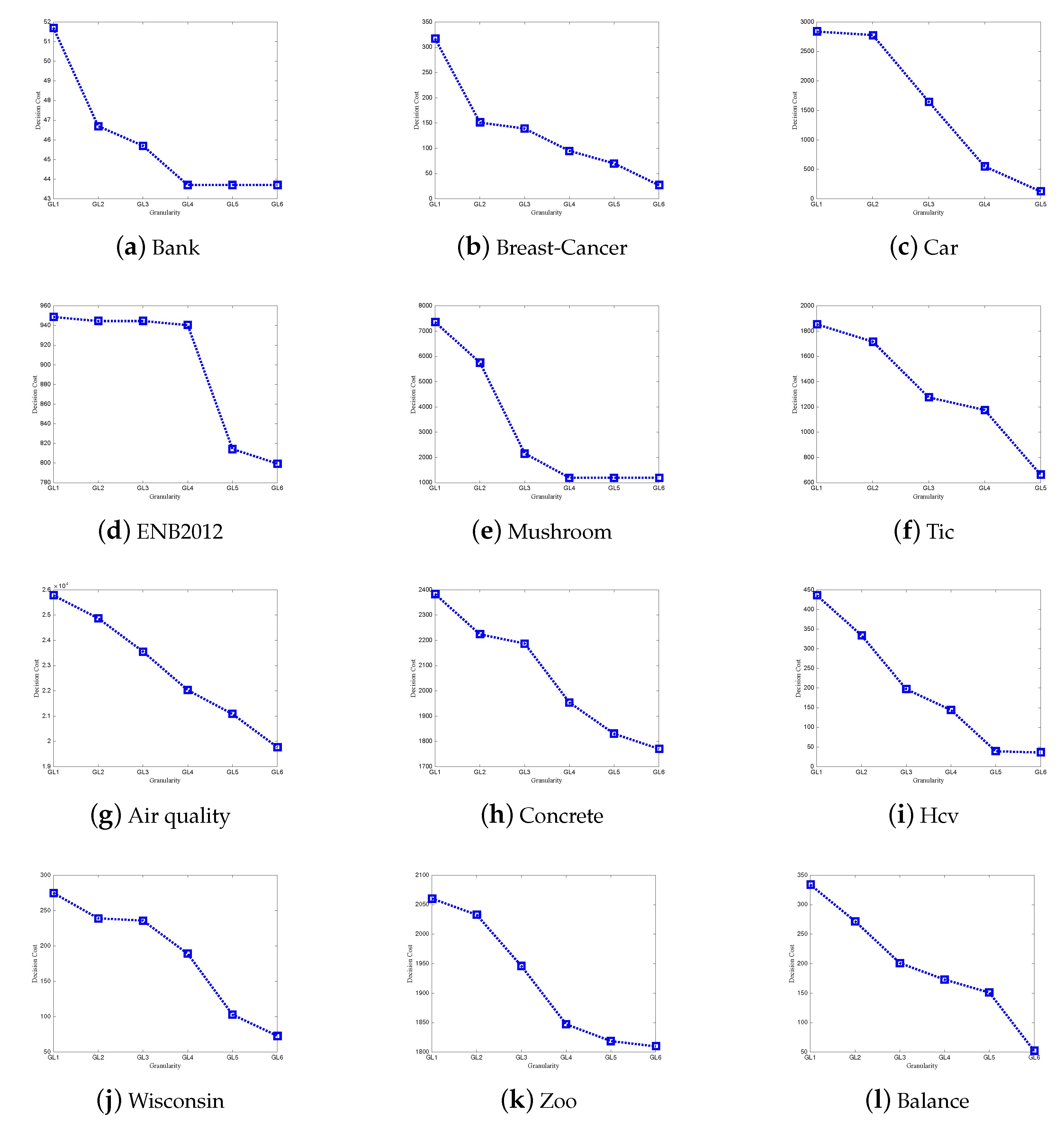
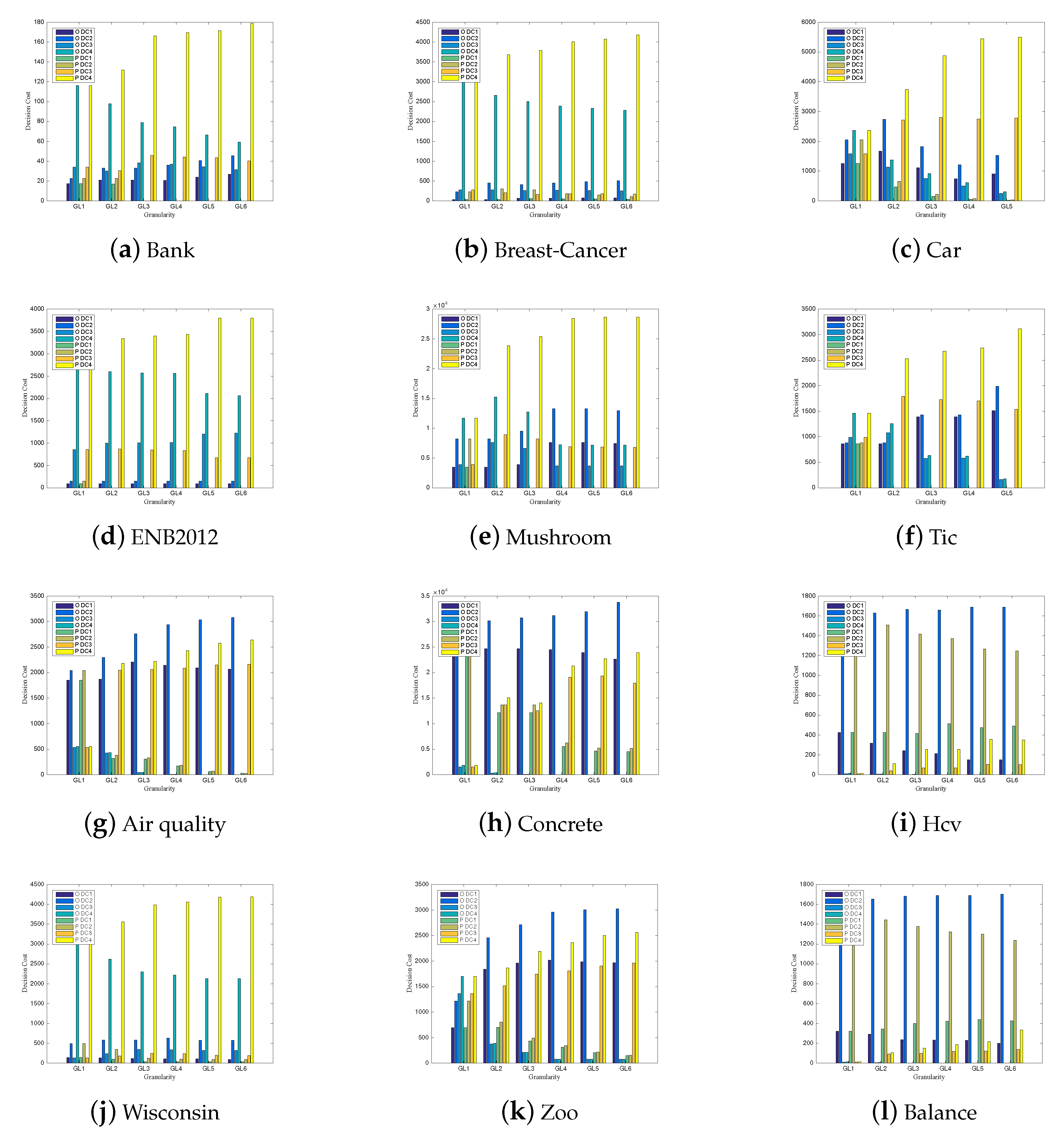
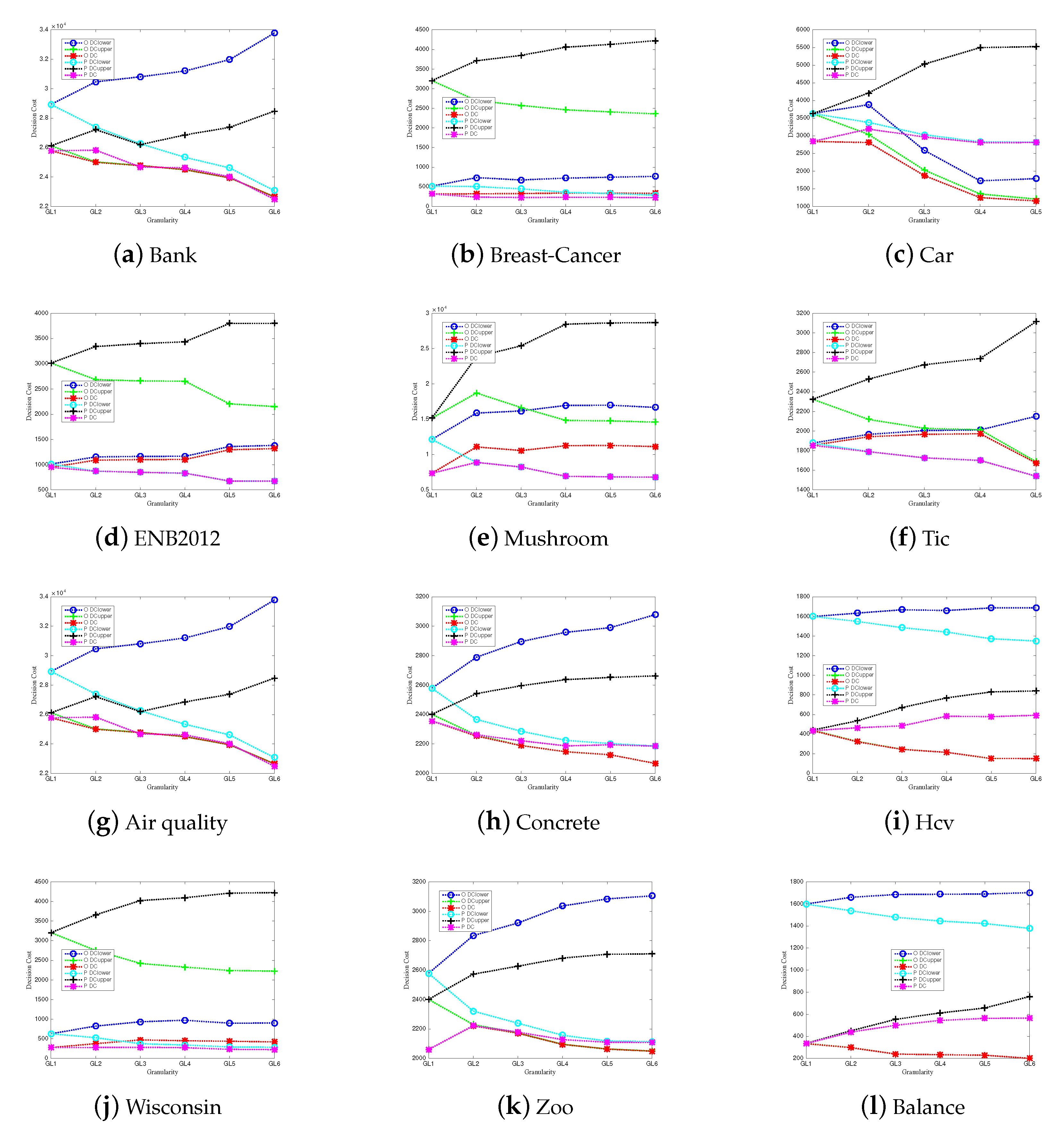
According to the above experiments, compared with the upper/lower approximation sets, we can conclude that the multigranulation approximations have the following advantages when applied to decision-making environments:

(1)

The misclassification costs of the approximation model monotonously decrease with the granularity being finer;

(2)

In multigranulation approximations, under different granular layers, the misclassification costs incurred by the equivalence classes in approximating X are less than or equal to the misclassification costs incurred by the equivalence classes when they do not characterize X in boundary region I of optimistic and pessimistic rough sets. Moreover, the misclassification costs incurred by equivalence classes when they do not characterize X are less than or equal to the misclassification costs incurred by the equivalence classes in approximating X in boundary region II of optimistic and pessimistic rough sets;

(3)

Compared with the upper/lower approximation sets, the misclassification costs of the multigranulation approximations are the least on each granularity.

7. Conclusions

In MGRS, optimistic and pessimistic upper/lower approximation boundaries are utilized to characterize uncertain concepts. They still cannot take advantage of the known equivalence classes to establish the approximation of an uncertain concept. To handle the problem, cost-sensitive multigranulation approximations of rough sets were constructed. Furthermore, an optimization mechanism of the multigranulation approximations is proposed, which selects the optimal approximation to obtain the minimum misclassification costs under the conditions. The case study shows that the proposed algorithm is capable of searching for a rational approximation under restraints. Finally, the experiments demonstrate that the multigranulation approximations possess the least misclassification costs. In particular, our models apply to the decision-making environment where each decision-maker is independent. Moreover, our models are useful for extracting decision rules from distributive information systems and groups of intelligent agents through rough set approaches [34,36]. Figure 7 presents a diagram that summarizes the works conducted in this paper. Herein, we present the process of the cost-sensitive multigranulation approximations of rough sets; according to different granulation mechanisms, our approach can be extended to uncertainty models, i.e., vague sets, shadow sets, and neighborhood rough sets. These results will be important to contribute to the progress of the GrC theory.

Our future work will focus on the following two aspects: (1) We hope to build a more reasonable three-way decision model based on our model from optimistic and pessimistic perspectives; (2) we wish to combine the model with the cloud model theory to extend our model to construct a multigranulation approximation model with bidirectional cognitive computing. This will offer more cognitive advantages and benefits in application fields with uncertainty from multiple perspectives, i.e., image segmentation, clustering, and recommendation systems.

References

1. Zadeh, L.A. Toward a theory of fuzzy information granulation and its centrality in human reasoning and fuzzy logic. Fuzzy Sets Syst. 1997, 90, 111–127. [Google Scholar] [CrossRef]
2. Bello, M.; Nápoles, G.; Vanhoof, K.; Bello, R. Data quality measures based on granular computing for multi-label classification. Inf. Sci. 2021, 560, 51–67. [Google Scholar] [CrossRef]
3. Pedrycz, W.; Chen, S. Interpretable Artificial Intelligence: A Perspective of Granular Computing; Springer Nature: Berlin/Heidelberg, Germany, 2021; Volume 937. [Google Scholar]
4. Li, J.; Mei, C.; Xu, W.; Qian, Y. Concept learning via granular computing: A cognitive viewpoint. IEEE Trans. Fuzzy Syst. 2015, 298, 447–467. [Google Scholar] [CrossRef] [PubMed]
5. Zadeh, L. Fuzzy sets. Inf. Control. 1965, 8, 338–353. [Google Scholar] [CrossRef] [Green Version]
6. Pawlak, Z. Rough sets. Int. J. Comput. Inf. Sci. 1982, 11, 341–356. [Google Scholar] [CrossRef]
7. Zhang, L.; Zhang, B. The quotient space theory of problem solving. In Proceedings of the International Workshop on Rough Sets, Fuzzy Sets, Data Mining, and Granular-Soft Computing, Chongqing, China, 26–29 May 2003; pp. 11–15. [Google Scholar]
8. Li, D.Y.; Meng, H.J.; Shi, X.M. Membership clouds and membership cloud generators. J. Comput. Res. Dev. 1995, 32, 15–20. [Google Scholar]
9. Colas-Marquez, R.; Mahfouf, M. Data Mining and Modelling of Charpy Impact Energy for Alloy Steels Using Fuzzy Rough Sets. IFAC-Pap. 2017, 50, 14970–14975. [Google Scholar] [CrossRef]
10. Hasegawa, K.; Koyama, M.; Arakawa, M.; Funatsu, K. Application of data mining to quantitative structure-activity relationship using rough set theory. Chemom. Intell. Lab. Syst. 2009, 99, 66–70. [Google Scholar] [CrossRef]
11. Santra, D.; Basu, S.K.; Mandal, J.K.; Goswami, S. Rough set based lattice structure for knowledge representation in medical expert systems: Low back pain management case study. Expert Syst. Appl. 2020, 145, 113084. [Google Scholar] [CrossRef] [Green Version]
12. Chebrolu, S.; Sanjeevi, S.G. Attribute Reduction in Decision-Theoretic Rough Set Model using Particle Swarm Optimization with the Threshold Parameters Determined using LMS Training Rule. Procedia Comput. Sci. 2015, 57, 527–536. [Google Scholar] [CrossRef] [Green Version]
13. Abdolrazzagh-Nezhad, M.; Radgohar, H.; Salimian, S.N. Enhanced cultural algorithm to solve multi-objective attribute reduction based on rough set theory. Math. Comput. Simul. 2020, 170, 332–350. [Google Scholar] [CrossRef]
14. Beaubier, S.; Defaix, C.; Albe-Slabi, S.; Aymes, A.; Galet, O.; Fournier, F.; Kapel, R. Multiobjective decision making strategy for selective albumin extraction from a rapeseed cold-pressed meal based on Rough Set approach. Food Bioprod. Process. 2022, 133, 34–44. [Google Scholar] [CrossRef]
15. Landowski, M.; Landowska, A. Usage of the rough set theory for generating decision rules of number of traffic vehicles. Transp. Res. Procedia 2019, 39, 260–269. [Google Scholar] [CrossRef]
16. Tawhid, M.; Ibrahim, A. Feature selection based on rough set approach, wrapper approach, and binary whale optimization algorithm. Int. J. Mach. Learn. Cybern. 2020, 11, 573–602. [Google Scholar] [CrossRef]
17. Zhang, Q.H.; Wang, G.Y.; Yu, X. Approximation sets of rough sets. J. Softw. 2012, 23, 1745–1759. [Google Scholar] [CrossRef]
18. Zhang, Q.H.; Wang, J.; Wang, G.Y. The approximate representation of rough-fuzzy sets. Chin. J. Comput. Jisuanji Xuebao 2015, 38, 1484–1496. [Google Scholar]
19. Zhang, Q.; Wang, J.; Wang, G.; Yu, H. The approximation set of a vague set in rough approximation space. Inf. Sci. 2015, 300, 1–19. [Google Scholar] [CrossRef]
20. Zhang, Q.H.; Zhang, P.; Wang, G.Y. Research on approximation set of rough set based on fuzzy similarity. J. Intell. Fuzzy Syst. 2017, 32, 2549–2562. [Google Scholar] [CrossRef]
21. Zhang, Q.H.; Yang, J.J.; Yao, L.Y. Attribute reduction based on rough approximation set in algebra and information views. IEEE Access 2016, 4, 5399–5407. [Google Scholar] [CrossRef]
22. Yao, L.Y.; Zhang, Q.H.; Hu, S.P.; Zhang, Q. Rough entropy for image segmentation based on approximation sets and particle swarm optimization. J. Front. Comput. Sci. Technol. 2016, 10, 699–708. [Google Scholar]
23. Zhang, Q.H.; Liu, K.X.; Gao, M. Approximation sets of rough sets and granularity optimization algorithm based on cost-sensitive. J. Control. Decis. 2020, 35, 2070–2080. [Google Scholar]
24. Yang, J.; Yuan, L.; Luo, T. Approximation set of rough fuzzy set based on misclassification cost. J. Chongqing Univ. Posts Telecommun. (Nat. Sci. Ed.) 2021, 33, 780–791. [Google Scholar]
25. Yang, J.; Luo, T.; Zeng, L.J.; Jin, X. The cost-sensitive approximation of neighborhood rough sets and granular layer selection. J. Intell. Fuzzy Syst. 2022, 42, 3993–4003. [Google Scholar] [CrossRef]
26. Siminski, K. 3WDNFS—Three-way decision neuro-fuzzy system for classification. Fuzzy Sets Syst. 2022, in press. [Google Scholar] [CrossRef]
27. Subhashini, L.; Li, Y.; Zhang, J.; Atukorale, A.S. Assessing the effectiveness of a three-way decision-making framework with multiple features in simulating human judgement of opinion classification. Inf. Process. Manag. 2022, 59, 102823. [Google Scholar] [CrossRef]
28. Subhashini, L.; Li, Y.; Zhang, J.; Atukorale, A.S. Integration of semantic patterns and fuzzy concepts to reduce the boundary region in three-way decision-making. Inf. Sci. 2022, 595, 257–277. [Google Scholar] [CrossRef]
29. Mondal, A.; Roy, S.K.; Pamucar, D. Regret-based three-way decision making with possibility dominance and SPA theory in incomplete information system. Expert Syst. Appl. 2023, 211, 118688. [Google Scholar] [CrossRef]
30. Yao, Y.Y. Symbols-Meaning-Value (SMV) space as a basis for a conceptual model of data science. Int. J. Approx. Reason. 2022, 144, 113–128. [Google Scholar] [CrossRef]
31. Qian, Y.H.; Liang, J.Y.; Dang, C.Y. Incomplete multigranulation rough set. IEEE Trans. Syst. Man-Cybern.-Part Syst. Humans 2009, 40, 420–431. [Google Scholar] [CrossRef]
32. Huang, B.; Guo, C.X.; Zhuang, Y.L.; Li, H.X.; Zhou, X.Z. Intuitionistic fuzzy multigranulation rough sets. Inf. Sci. 2014, 277, 299–320. [Google Scholar] [CrossRef]
33. Li, F.J.; Qian, Y.H.; Wang, J.T.; Liang, J. Multigranulation information fusion: A Dempster-Shafer evidence theory-based clustering ensemble method. Inf. Sci. 2017, 378, 389–409. [Google Scholar] [CrossRef]
34. Liu, X.; Qian, Y.H.; Liang, J.Y. A rule-extraction framework under multigranulation rough sets. Int. J. Mach. Learn. Cybern. 2014, 5, 319–326. [Google Scholar] [CrossRef]
35. Liu, K.; Li, T.; Yang, X.; Ju, H.; Yang, X.; Liu, D. Hierarchical neighborhood entropy based multi-granularity attribute reduction with application to gene prioritization. Int. J. Approx. Reason. 2022, 148, 57–67. [Google Scholar] [CrossRef]
36. Qian, Y.H.; Liang, X.Y.; Lin, G.P.; Guo, Q.; Liang, J. Local multigranulation decision-theoretic rough sets. Int. J. Approx. Reason. 2017, 82, 119–137. [Google Scholar] [CrossRef]
37. Qian, Y.H.; Zhang, H.; Sang, Y.L.; Liang, J. Multigranulation decision-theoretic rough sets. Int. J. Approx. Reason. 2014, 55, 225–237. [Google Scholar] [CrossRef]
38. Xu, W.; Yuan, K.; Li, W. Dynamic updating approximations of local generalized multigranulation neighborhood rough set. Appl. Intell. 2022, 52, 9148–9173. [Google Scholar] [CrossRef]
39. Sun, L.; Wang, L.; Ding, W.; Qian, Y.; Xu, J. Feature selection using fuzzy neighborhood entropy-based uncertainty measures for fuzzy neighborhood multigranulation rough sets. IEEE Trans. Fuzzy Syst. 2020, 29, 19–33. [Google Scholar] [CrossRef]
40. She, Y.H.; He, X.L.; Shi, H.X.; Qian, Y. A multiple-valued logic approach for multigranulation rough set model. Int. J. Approx. Reason. 2017, 82, 270–284. [Google Scholar] [CrossRef]
41. Li, W.; Xu, W.; Zhang, X.Y.; Zhang, J. Updating approximations with dynamic objects based on local multigranulation rough sets in ordered information systems. Artif. Intell. Rev. 2021, 55, 1821–1855. [Google Scholar] [CrossRef]
42. Zhang, C.; Li, D.; Zhai, Y.; Yang, Y. Multigranulation rough set model in hesitant fuzzy information systems and its application in person-job fit. Int. J. Mach. Learn. Cybern. 2019, 10, 717–729. [Google Scholar] [CrossRef]
43. Hu, C.; Zhang, L.; Wang, B.; Zhang, Z.; Li, F. Incremental updating knowledge in neighborhood multigranulation rough sets under dynamic granular structures. Knowl.-Based Syst. 2019, 163, 811–829. [Google Scholar] [CrossRef]
44. Hu, C.; Zhang, L. Dynamic dominance-based multigranulation rough sets approaches with evolving ordered data. Int. J. Mach. Learn. Cybern. 2021, 12, 17–38. [Google Scholar] [CrossRef]
Figure 1. The approximation of rough sets (surrounded by the broken line).
Electronics 11 03801 g001
Figure 2. The granules subdivided in B N 1 ( X ) and B N 2 ( X ) of the cost-sensitive approximation model of rough sets. And all the red circles in the figure represent the set X. In addition, (a) shows the case 1 in which the granules are subdivided in B N 1 ( X ) ; (b) shows the case 2 in which the granules are subdivided in B N 1 ( X ) ; (c) shows the case 1 in which the granules are subdivided in B N 2 ( X ) ; (d) shows the case 2 in which the granules are subdivided in B N 2 ( X ) .
Electronics 11 03801 g002
Figure 3. The optimal granularity selection of the optimistic multigranulation approximation. And the red circles in the figure represent the set X.
Electronics 11 03801 g003
Figure 4. The misclassification cost with the changing granularity on each dataset.
Electronics 11 03801 g004
Figure 5. The misclassification cost of two boundary regions under different granularities.
Electronics 11 03801 g005
Figure 6. The misclassification costs of i = 1 m A i O ̲ ( X ) , i = 1 m A i O ¯ ( X ) , i = 1 m A i O ( X ) , i = 1 m A i P ̲ ( X ) , i = 1 m A i P ¯ ( X ) , i = 1 m A i P ( X ) with the changing granularity of each dataset.
Electronics 11 03801 g006
Figure 7. Diagram of works conducted in this paper.
Electronics 11 03801 g007