Article

Research on a Sowing Depth Detection System Based on an Improved Adaptive Kalman Filtering Method

College of Engineering, Heilongjiang Bayi Agricultural University, Daqing 163319, China
*
Author to whom correspondence should be addressed.
Electronics 2022, 11(22), 3802; https://doi.org/10.3390/electronics11223802
Submission received: 26 October 2022 / Revised: 14 November 2022 / Accepted: 17 November 2022 / Published: 18 November 2022

Abstract

:
The current real-time detection of sowing depth has the problems of low detection accuracy and poor reliability. After analyzing the movement mechanism of the sowing monomer parallel four-bar linkage, an improved adaptive Kalman filtering method for sowing depth detection is proposed. The method uses two MPU6050 attitude sensors. The difference between the rotation angle of the parallel four-bar linkage and the attitude angle of the sowing monomer is used as the relative rotation angle of the parallel four-bar linkage relative to the sowing monomer. The sowing monomer parallel four-bar linkage has the characteristics of up–down translation, and sowing depth changes can be obtained by converting the angle data. By using moving average filter, particle filter, Kalman filter, and improved adaptive Kalman filter to fuse the data of MPU6050 in two positions and perform MATLAB simulation, the average mean squared errors of the above four filtering algorithms are 0.12645, 0.05545, 0.03785, and 0.0189, respectively. In the end, the experiment of sowing depth detection was carried out, and it was found that the improved adaptive Kalman filter algorithm detects the smallest sowing depth mean squared error, which is 0.0636, and the algorithm can track data changes better. At the same time, it is more adaptable to noise and obtains an ideal filtering effect.

1. Introduction

Sowing quantity, plant spacing, and sowing depth are the main indicators for evaluating the sowing quality of seeders [1,2,3]. The proper sowing depth allows the seeds to have full contact with the soil. It also allows the seeds to fully absorb water and nutrients from the soil. Sowing depth detection is an indispensable part of the active control system of sowing depth.
In terms of sowing depth detection, due to the increased promotion of no-tillage sowing in recent years, the process of sowing depth detection has been affected by surface residues and soil compaction, resulting in a decrease in detection accuracy and large data fluctuations, this leading to a decrease in the control accuracy of the active control system for sowing depth. Therefore, there is a need to investigate sowing depth detection methods in order to obtain sowing depth data with higher detection accuracy.
Zhou Shuhui et al. [4] used the pressure value of the FLEX flexible sensor as the basis for judging the sowing depth of the sowing monomer. This method must destroy the depth-limiting wheel during the installation process, which is difficult to install. Close contact can easily damage the sensor and affect the detection accuracy. Gao Yuan et al. [5,6] realized the detection of the sowing depth by installing an angle sensor on the shaft of the depth-limiting arm. This method avoids damage to the sowing monomer structure and enhances the generality. However, since the angle sensor is installed in the depth-limiting arm, the rotary shaft vibrates considerably, and proper filtering is not performed, resulting in high data volatility, which affects subsequent sowing depth control. It is necessary to select an appropriate filtering method according to the actual situation, and this system is less popular. Jiang Xiaohu et al. [7]. used laser sensors and ultrasonic sensors to measure tillage depth and used a combination of Kalman filtering and weighted average filtering for filtering and data fusion. The resulting tillage depth data are more stable and more accurate. However, the Kalman filter requires an accurate mathematical model in the calculation process and therefore still has many shortcomings in a noisy and changing field environment. It is unable to effectively track noise variations. Although there are some differences in the way tillage depth and sowing depth are measured, the measurements of the two operations can, to a certain extent, be used in conjunction with each other.
Suomi and Oksanen [8] used the angle sensor of the planter frame to measure the rotation angle of the opener relative to the frame and the rotation angle of the lateral support wheel relative to the frame. The values collected by the above sensors were converted into sowing depth, and the moving average filter algorithm was used to measure the variation of sowing depth. This method is less likely to cause the sensor to vibrate during detection, but it is still inadequate for data filtering. The moving average filter algorithm smooths the data to a certain extent, but the noise was calculated in the filtering process, resulting in poor data accuracy.
After the above analysis of the study, it was found that the sensor should be installed in a location where the sensor is less subject to vibration to avoid damage to the sowing monomer. In terms of sensor data filtering, a better filtering algorithm that is more adaptable to noise should be selected.
In view of the above problems, the MPU6050 angle sensor is used in this study to detect the rotation angle of the parallel four-bar linkage of the sowing monomer as the basis for the detection of the sowing depth [9]. This method does not damage the single structure of the sowing, has a low installation difficulty, and is suitable for large-scale usage. In addition, the parallel four-bar linkage of the sowing monomer causes less vibration during operation and has less impact on the accuracy of data collection than the two positions of the sowing monomer’s depth-limiting wheels and arms. The built-in acceleration sensor and gyro sensor of the MPU6050 can perform direct and indirect angle detection, respectively [10,11,12,13]. However, the acceleration sensor is susceptible to vibration interference during detection, and the gyroscope sensor generates cumulative errors during the integral operation of the angle. Therefore, a suitable filtering algorithm must be selected for data fusion. In the field of data fusion, Bayesian algorithm, moving average filter algorithm, standard Kalman filter algorithm, etc., are generally used [14,15,16]. In this study, moving average filter [17], particle filter [18,19,20,21], Kalman filter [22,23,24,25], and improved adaptive Kalman filter algorithm [26,27,28] are used to conduct the experiments. Finally, it was found that the improved adaptive Kalman filter can adaptively adjust the noise during the filtering process. The anti-interference ability of the algorithm was greatly improved and avoids reliance on old data after long runs. Compared to the other algorithms in this paper, we obtained more ideal results.
The rest of this paper is organized as follows. Section 2 introduces the detection principle and hardware structure of the sowing depth detection system. Section 3 introduces the data fusion algorithm and establishes the state equation. Section 4 conducts simulation experiments on the data fusion algorithm and analyzes and summarizes the results. The sowing monomer movement experiment was carried out on the system, and the experimental results were analyzed. Section 5 summarizes the entire paper.

2. Materials and Methods

2.1. System Structure

The sowing depth detection system is mainly composed of a sowing monomer, MPU6050 angle sensor, STM32F103RCT6 microcontroller, 5V power supply, and other structures. The working frequency of the STM32F103RCT6 microcontroller is 72 MHZ, meaning it can quickly process sensor data. The microcontroller communicates with the MPU6050 sensor through the I2C protocol. The output frequency of sensor data is 100 HZ, which can meet the data collection speed of the sensor working in the field and obtain enough data. The static error of sensor operation is ±0.2°. Its overall structure and the sensor installation position are shown in Figure 1.

2.2. Working Principle

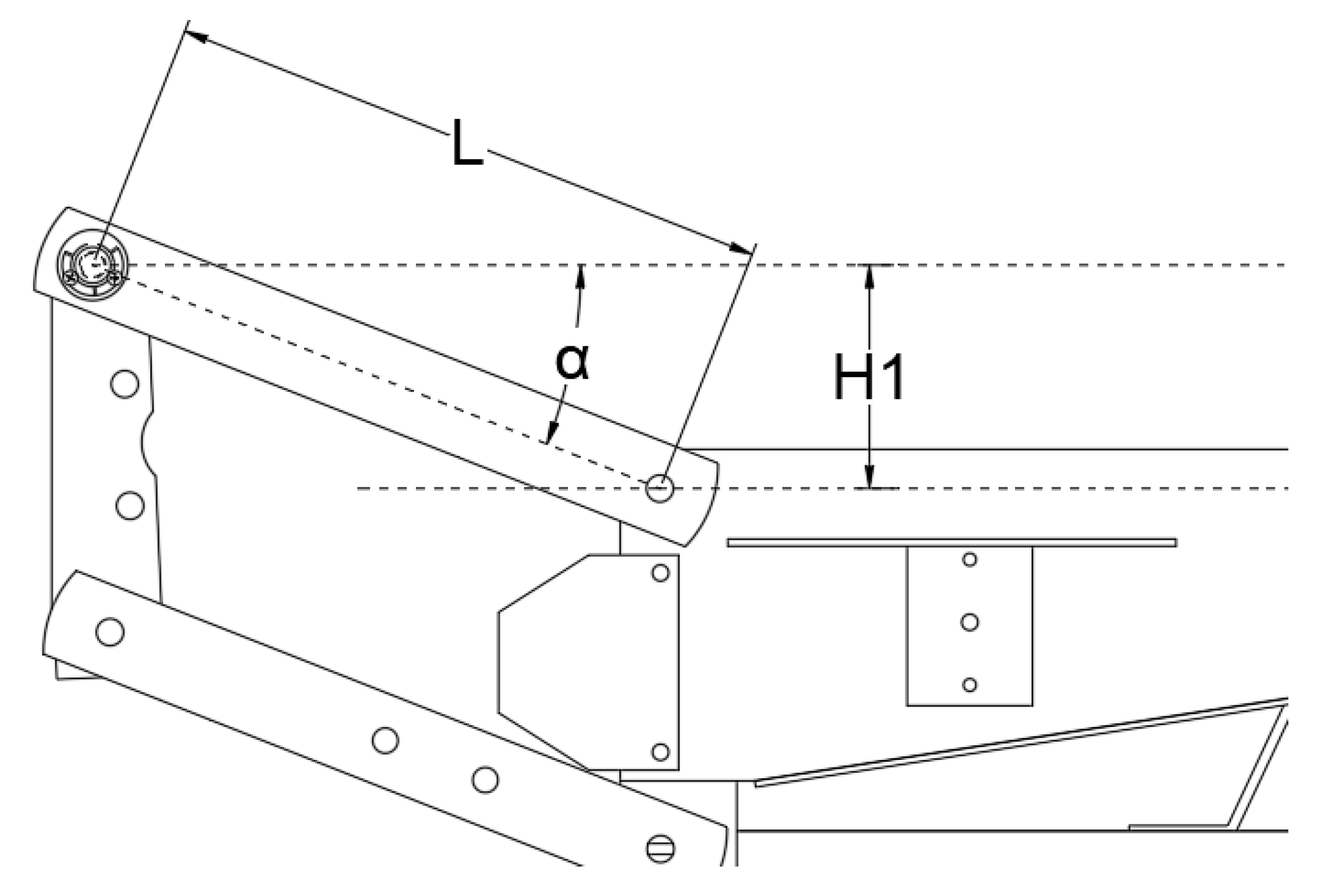
The working principle can be obtained from the motion characteristics of the sowing monomer parallel four-bar linkage. The sowing monomer parallel four-bar linkage rotates up and down with the fixed beam at the front of the rack as the axis. The upper rod and the lower rod always move in parallel so that the sowing monomer basically maintains the up-and-down translation when working in the field, ensuring the consistency of the sowing depth. The sensor detection principle of the MPU6050 is accelerometer detection and gyroscope detection. The angle measured by the acceleration sensor is the rotation angle of the acceleration sensor relative to the ground. Therefore, in addition to the rotation angle of the parallel four-bar linkage of the sowing monomer, the attitude angle of the sowing monomer itself must be considered. The difference between the two is the rotation angle of the parallel four-bar linkage relative to the sowing monomer. The schematic diagram of the rotation angle detection of the sowing monomer parallel four-bar linkage is shown in Figure 2. The length of the sowing monomer parallel four-bar linkage is 40 cm. The rotation angle of the parallel four-bar linkage is used to obtain the distance of the downward movement of the sowing monomer compared to the horizontal position of the parallel four-bar linkage. Subtracting this distance from the distance that the sowing monomer moves downwards when the sowing depth is 0 gives us the sowing depth at this point. The formula for calculating the seeding depth H is:
H 1 = sin α × L .
H = H 1 H 0  
where α is the parallel four-bar linkage rotation angle, L is the length of the sowing monomer parallel four-bar linkage, H 1 is the distance of the downward movement of the sowing monomer compared to the horizontal position of the parallel four-bar linkage, and H 0 is the distance that the sowing monomer moves downwards when the sowing depth is 0.

3. Data Fusion Algorithm

3.1. Moving Average Filter

Moving average filtering (MAF) has two steps. The first is to establish a data queue and store the data in order—first in, first out. The data length is fixed to N. The algorithm implements data update by using a window of length N to store and retrieve data; the second is to calculate the average value. The filter output is always guaranteed to be the average of N updated data points.
When encountering a signal with interference, if the interference is random, arithmetic moving average filtering can be used. The advantage of this filtering method is its simplicity. It has a strong inhibitory effect on high-frequency oscillation. The disadvantage is that calculating the average will also calculate the impulse disturbance. The algorithm has low sensitivity and accuracy, which come at the expense of memory. In general, the effect of the filter is also different when N is different. The larger the N, the larger the amount of data required and the better the smoothness. At the same time, the lower the memory, the higher the sensitivity. The moving average filter formula is as follows:
z ¯ = 1 N i = 1 N z i  
where z ¯ is the arithmetic mean of N sampled values and z i is the ith sampled value.

3.2. Particle Filter

Particle filter (PF) achieves the Bayesian estimation filter in another form through the nonparametric Monte Carlo simulation method. Particle filter describes prior and posterior information in time domain in the form of samples, not functions. The sample form adopted is called the sampling point, also called “particle”.
The algorithm approximately estimates the actual probability distribution by adjusting the proportion of each “particle” weight and the position of sample collection. When the number of samples collected approaches infinity, the function of posterior information probability density is basically the same as that of the Monte Carlo simulation. We believe that the two forms are statistically equivalent. At this time, the mean value of particles can be used as an estimate of the system. An optimal estimate is used to approximate nonlinearity. This method is not restricted by linear and Gaussian distribution in the field of mathematics. In principle, it can be used for the optimal estimation of the state of any nonlinear, non-Gaussian stochastic system.
The particle filter algorithm, as a whole, includes three steps: time update, observation update, and resampling. It is known that the weight of N sampled particles at k − 1 is 1/N. In the time updating phase, the state of each particle at time k is predicted by the state equation of the system. The weight w k i of the particles is updated in the observation update stage, the weight of particles with significant weight is reset in the resampling stage, and the particle weight is reset to 1/N.
The calculation process of particle filter algorithm is divided into six steps:
Step 1: Initialize the particles.
When k = 0, take N sampling points x 0 i , i = 1, 2, 3,..., N;
where x 0 i is the state of the ith particle at time 0.
Step 2: Perform importance sampling to obtain sampling particles:
x ˜ 0 : k i ~ q ( x k | x 0 : k 1 i , z 1 : k )  
x ˜ 0 : k i = x 0 : k i , x ˜ k i  
Step 3: Update the weight:
w k i = w k 1 i p ( z k | x k i ) p ( x k i | x k 1 i ) q ( x k i | x 0 : k 1 i , z 1 : k )  
The above equation is simplified as follows:
w k i = w k 1 i p ( z k | x k i )  
where w k i is the weight of the ith particle at time k.
Step 4: Normalize weight:
t = i = 1 N w k i  
w k i = w k i t  
Step 5: Perform resampling, with the normalized weight:
w k i = 1 / N  
Step 6: Update the results.
Obtain output set: x 0 : k i : i = 1 , 2 , 3 , , N and calculate the updated posterior probability expectation using this set.

3.3. Kalman Filter

In the 1960s, Kalman published a paper that would have far-reaching consequences for later generations. In this paper, Kalman systematically described the method by using recursion. Through the operation, the original discrete data are subjected to linear filtering to obtain the desired result. The Kalman filter (KF) provides an autoregressive algorithm for processing data. This algorithm is highly optimized and has been adopted by many researchers. The algorithm has an obvious effect on the discrete filtering of a linear system and has been widely used for more than 30 years. Applications include aircraft orbit correction, robotic system control, radar systems, and missile tracking.
The Kalman filter algorithm is a recursive estimation algorithm. It analyzes and predicts the following state based on the previous state. The premise of this algorithm is to know the estimated value of the previous state first. The specific value of the current state is also needed to match the estimated value for prediction. This results in a relatively stable value. A measurement of the current state is also required. Based on these two values, we can roughly estimate the estimated value of the current state. There is no need to record too much historical information, as we only need to know the previous state and the next state prediction can be used. A very significant advantage of the Kalman filter is that it is itself a filter that operates in the time domain. Compared to other filters, the Kalman filter simplifies the process of designing a method in the frequency domain and then transferring it to the time domain to be implemented.
The Kalman filter is a filter based on state and observation equations. Because the algorithm input contains process noise and measurement noise, in order to make the output value closer to the real value, the system adopts the method of minimum root mean square error to output the target value. The specific implementation method is to predict the next state value and correct and update the relevant parameters through the currently known state information. An iterative algorithm is used to obtain the optimal estimate. In essence, it is a process of constantly using new information to modify the posterior distribution, thereby approximating the optimal distribution. The schematic diagram of the Kalman filter algorithm is shown in Figure 3.
For a discrete system, first establish the state and observation equations with noise:
x k = A x k 1 + B u k 1 + w z k 1 = H x k 1 + v
where x k 1 is the value of the system state variable x at time k − 1, u k 1 is the input of the system at time k − 1, z k 1 is the output of the system at time k − 1, A is the system state transition matrix,   B is the system input matrix, H is system output matrix, w is the process noise of the system and v is the measurement noise of the system.
In the calculation process, it is considered that the noise w and v both conform to the normal distribution, w ~P(0, Q), v ~P(0, R), where Q and R represent the covariance matrix and the size of this value affects the filtering result.
The Kalman filter first predicts the next state, uses the output at the previous moment as the system input at the next moment, and then updates the estimated value. The eight steps correspond to the eight equations, and the relevant parameters are calculated to cause the estimated value to approach the real value and to obtain the optimal output.
The filter algorithm is used to estimate the target state value at time k. The basic process and core update equations of the KF algorithm are as follows:
Step 1: Initialization: Initialize the state variable x and the error covariance matrix P k at time k − 1:
Step 2: State prediction:
x ^ k = A x ^ k 1 + B u ^ k 1  
where x ^ k is the estimated value of the depth detection device at time k.
Step 3: Covariance matrix prediction:
P k = A P k 1 A T + Q  
where P k , i the prediction covariance at time k, P k 1 is the covariance of system state at k − 1 time, and Q is the system process noise covariance matrix.
Step 4: Measurement and prediction:
z ^ k = H x ^ k  
where z ^ k is the measured predictive value at time k.
Step 5: Kalman gain update:
K k = P k H T H P k H T + R i 1  
where K k is the Kalman gain at time k and R is the observation noise variance covariance matrix.
Step 6: Update with the new information.
δ k = z k H x ^ k  
where δ k is the filtering innovation term at time k and z k is the measured value of the sensor at time k.
Step 7: Update the target status:
x ^ k = x ^ k + K k δ k  
where x ^ k , i is the optimal estimate of the system at time k.
Step 8: Update the covariance matrix:
P k = I K k H P k  
where I is the identity matrix and P k is the estimated value of covariance at time k.

4. Experiment and Result Analysis

4.1. Simulation Results

In the system simulation software, because MATLAB has a variety of simulation models and is convenient for programming, this paper used MATLAB for the numerical simulation. In order to carry out the MATLAB simulation successfully, the system state equation and observation equation needed to be constructed first. The MPU6050 sensor state equation and observation equation construction method used in this paper were as follows. The MPU6050 sensor has two angle calculation methods. The first is to integrate the angular velocity output by the gyroscope. The second is to directly obtain the output value of the sensor accelerometer as the angle value. Therefore, the MPU6050 sensor takes the integration of the gyroscope output angular rate as the state equation and the direct output of the accelerometer as the observation equation. In the entire process of measurement, the weights of gyroscope and accelerometer are constantly adjusted. That is, the predicted angle at time k is approximately the static angle at time k − 1 plus the angular rate measured by the gyroscope times the time. The static drift of the gyro at time k is approximately the same as that at time k − 1, i.e., β k = β k 1 . The angle measured by the accelerometer is not related to the gyro drift β k , so the measurement system parameters are 1 0 .
The specific model can be expressed as:
α k = α k 1 + ω k 1 + β k 1 + w k 1 d t  
where α k is the prediction angle at time D, ω k 1 is the angular velocity of gyroscope at k − 1, β k 1 is the static drift at k − 1, w is the measurement noise, and d t is the measurement time.
The state equation of the system can be obtained from the above relations:
α ^ k β ^ k = 1 T s 0 1 α k 1 β k 1 + T s 0 U k  
The system measurement equation is:
z k = 1 0 α k β k + v k  
where U k is the gyroscope output, T s is the sampling time, z k is the measurement angle of the accelerometer, and v k is the acceleration measurement noise.
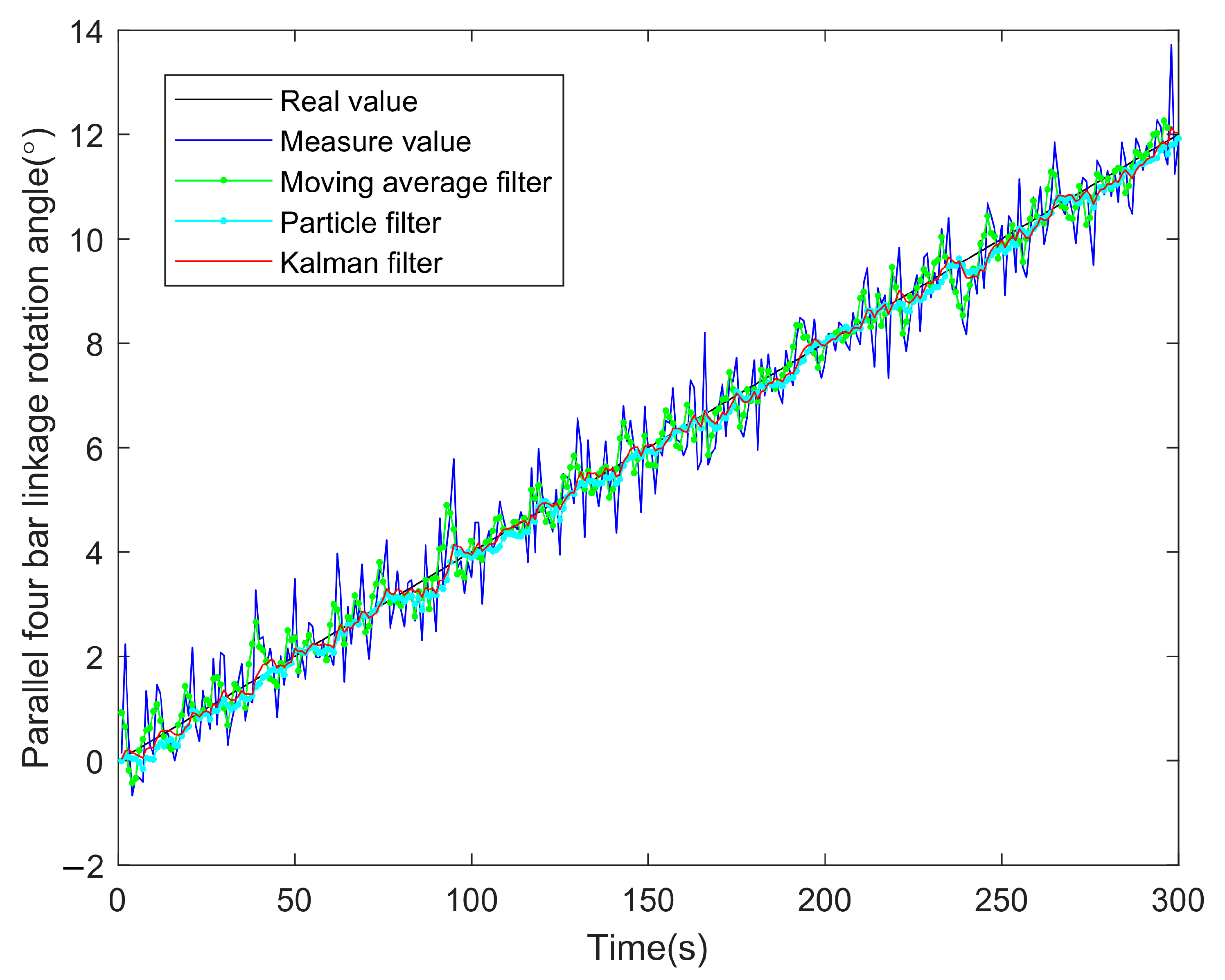
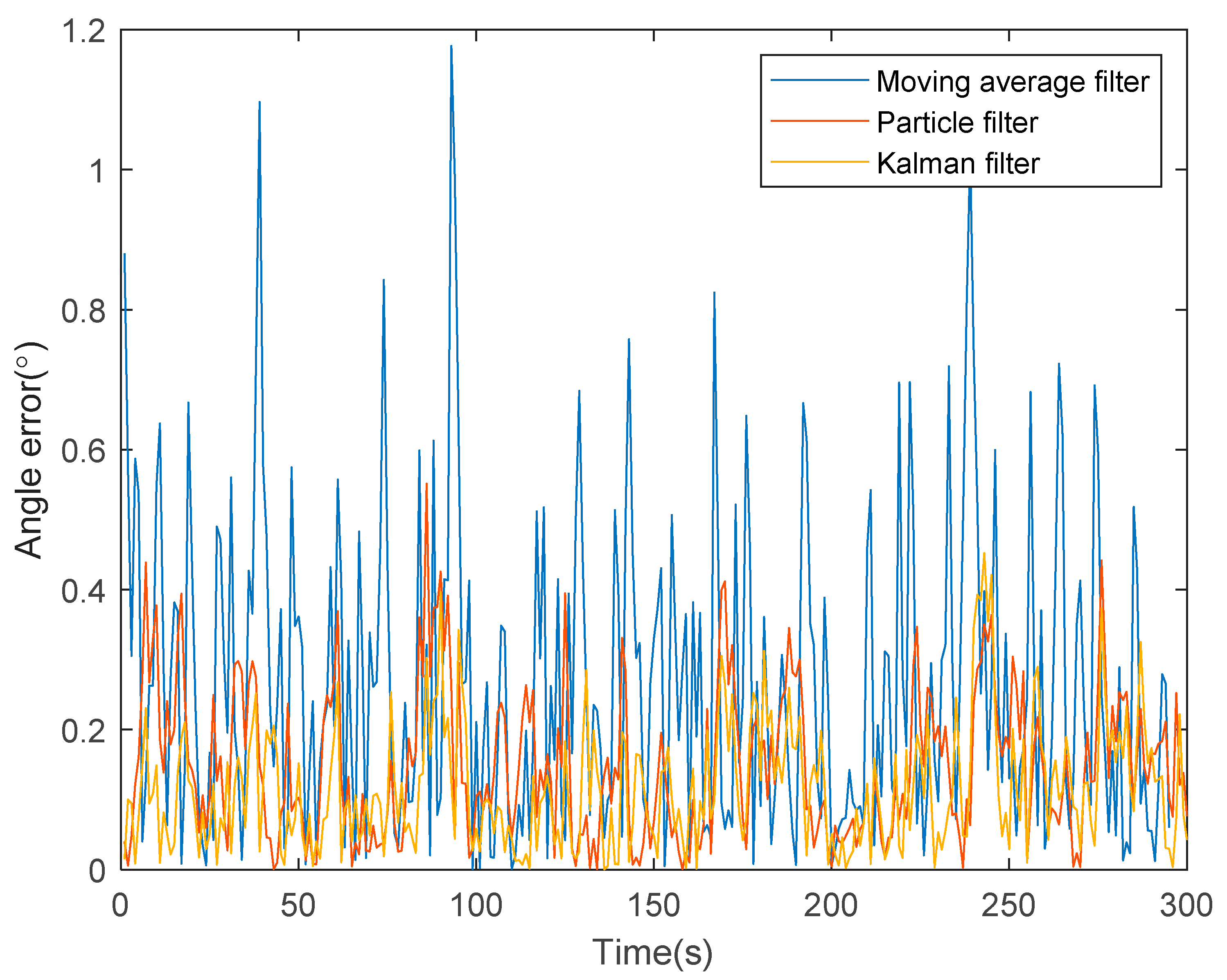
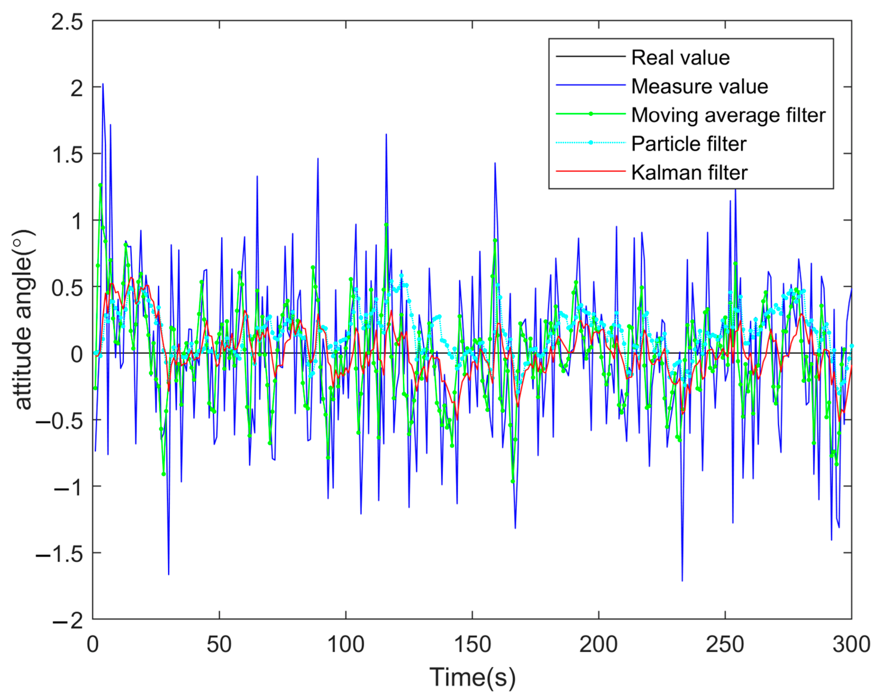
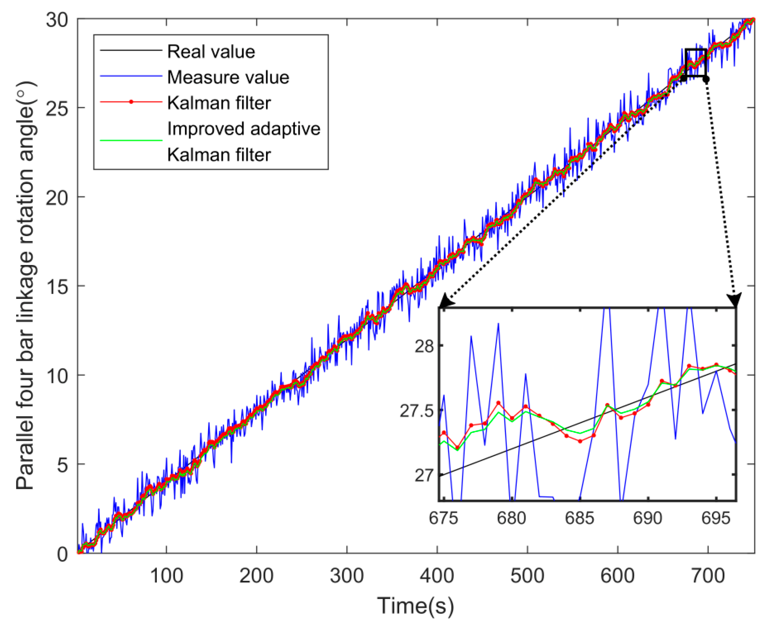
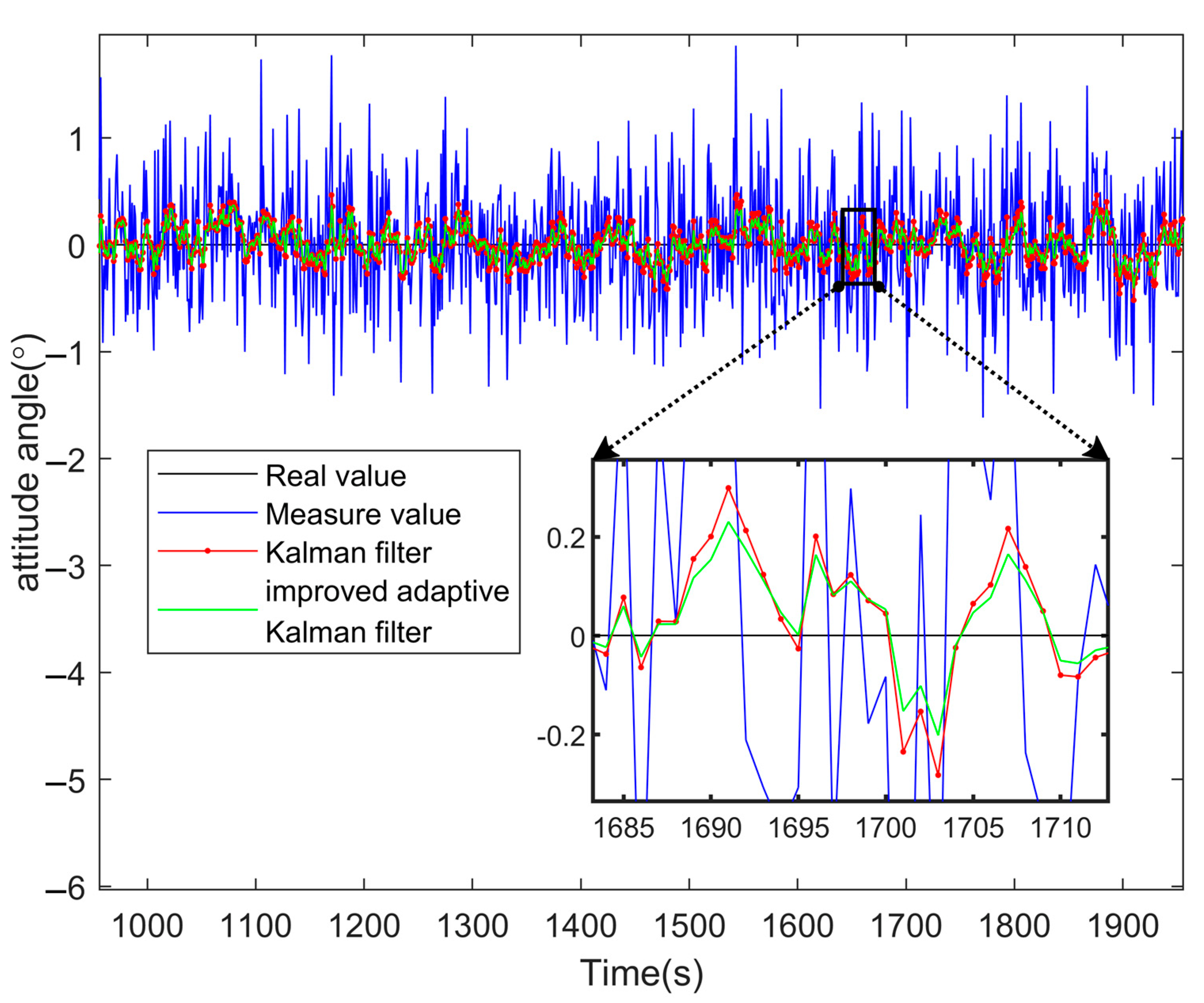
This study assumed that the inclination angle of the sowing monomer parallel four-bar linkage increases slowly with time. The attitude angle of the sowing monomer remains unchanged. We simulated the situation of the monomer when working in the field. The simulation time was 300 s. Real value is the real angle value generated by the MATLAB simulation, and measure value is the angle value of the sensor measurement generated by MATLAB. The other curves are the filtered angle values of the corresponding algorithms. The parallel four-bar linkage rotation angle simulation is shown in Figure 4, the algorithm error is shown in Figure 5, the sowing monomer attitude angle simulation is shown in Figure 6, and the algorithm error is shown in Figure 7.
It can be seen from the above simulation results that the Kalman filter algorithm has the best effect among the three filtering algorithms, which is closer to the real value in the simulation process, with an average MSE (mean squared error) of 0.0413; followed by particle filtering, with an average MSE of 0.05325; and finally, the moving average filter had the worst effect, with an average MSE of 0.1251. The algorithm simulation MSE is shown in Table 1.

4.2. Adaptive Kalman Filter

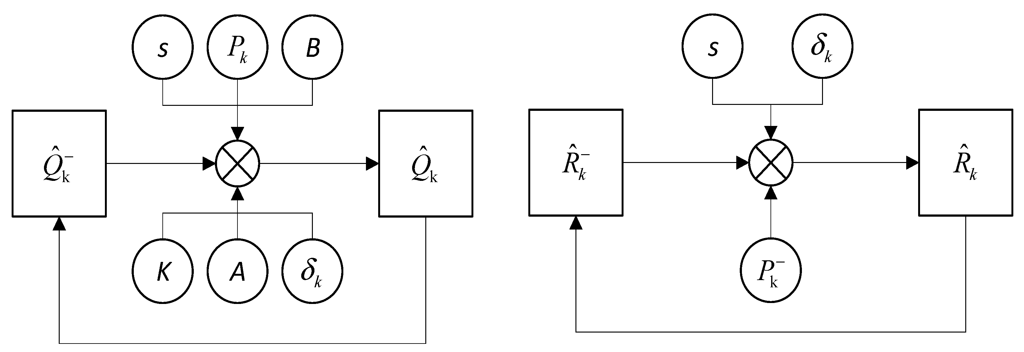
Although, in the above simulation results, the Kalman filter played a certain filtering effect, it can be seen from the simulation results that, when the measured data fluctuates greatly, the Kalman filter still has a large error. The Kalman filter needs to know the determined system noise covariance Q and measurement noise covariance R first. The accuracy of noise acquisition has a great relationship with the filtering results. In the actual system, it is difficult to know the exact Q and R values due to the complexity of the field environment, which makes the filtering result less accurate. Therefore, this paper decided to use the Sage–Husa adaptive Kalman filter. The Sage–Husa adaptive Kalman filter enhances noise adaptation. While using the observation data for recursive filtering, the forgetting factor is used to continuously estimate and correct the inaccurate parameters of the model and the noise covariance matrix. In this way, it can adapt to the interference of the environment and the time variations in the filtering process. This method can improve filtering accuracy and reduce state estimation errors, achieving a good filtering effect. The principle of the Sage–Husa adaptive Kalman filter algorithm is shown in Figure 8.
When using the Kalman filter to iterate the state equation, a time-varying noise statistical estimator is introduced according to the characteristics of the state equation itself.
First, replace Q and R in the formula with the estimated values Q ^ k and R ^ k , respectively, and then introduce the following equations:
G = B T B 1 B T  
Q ^ k = 1 α k 1 Q ^ k + α k 1 G K k δ k δ k T K k T + P k A P k 1 A T G T  
R ^ k = 1 α k 1 R ^ k + α k 1 δ k δ k T P k  
where α k and 1 − α k are used for index weighting. The so-called index weighting refers to the different weight coefficients that are attributed to the old data and the new data so that the new data plays a considerable role in the estimation and the old data is gradually forgotten. The weight coefficient subscribes to the law of negative exponential function.
When the forgetting factor s is considered according to 0 < s < 1, there is the following equation:
s 0 + s 1 + s k 1 = 1 s k / 1 s  
s 0 + s 1 + s k 1 1 s / 1 s k = 1  
To meet the requirements of the weight coefficient sequence, the following adjustments are made for α k :
α k = 1 s / 1 s k  
0 < s < 1  
where the forgetting factor s should be determined by experiments and is generally 0.95 or 0.99.
The suboptimal unbiased maximum a posteriori (MAP) noise statistical estimator of the Sage–Husa algorithm used above is simple to calculate. The algorithm can simultaneously estimate the system noise covariance and the measurement noise covariance. However, when the system order is high, filter divergence is prone to occurring. When the filter divergence occurs, it always accompanies and loses positive semi-definiteness and positive definiteness. The direct reason is that when the system adopts the subtraction algorithm to meet the requirement of unbiased estimation, filter divergence is caused.
Since the above time-varying noise statistical estimators diverge easily, the following biased estimation formula is adopted:
Q ^ k = 1 α k 1 Q ^ k + α k 1 G K k δ k δ k T K k T + P k G T  
R ^ k = 1 α k 1 R ^ k + α k 1 δ k δ k T  
Because the statistical characteristics of noise cannot be accurately known in advance, in the filtering process of the system, the adaptive Kalman filtering method is adopted, and the covariance matrix P gradually approaches zero after the system runs for a period of time. This is due to the fact that the state estimation is too dependent on previous data, which leads to filter divergence. In order to solve this problem, we attempted to reduce the influence of the old measurement value and strengthen the weight of the new observation value. In the literature, an adaptive algorithm of attenuation factor was proposed, whose formula is as follows:
P k = λ k A P k 1 A T + Q ^ k  
where λ k is the attenuation factor.
The value of attenuation factor λ k is as follows:
λ k = λ k λ k > 1 1     λ k 1  
λ k = δ k T δ k t r N k t r M k  
N k = H Q ^ k H T + R ^ k  
M k = H A P k 1 A T H T  
In each iterative filtering process, if the estimation error decreases, the method achieves λ k = 1 when λ k ≤ 1, which is the simplified Sage–Husa filtering. If the estimation error increases, which makes λ k increase when λ k > 1, the prediction error matrix P k increases, which increases the state gain matrix K k . By increasing the weight of innovation, we can reduce the impact of observation on estimation, making λ 1 = 1 .
Since it takes a certain amount of time for the adaptive factor to take effect, the adaptive algorithm is not very different from the ordinary algorithm in the early stage of the filtering algorithm, so the simulation time is increased. Previous research has found that the KF algorithm is better than the MAF and PF algorithms. Therefore, this simulation only compared the KF and improved adaptive Kalman filter (IAKF) algorithms. The algorithm simulation diagrams are shown in Figure 9, Figure 10, Figure 11 and Figure 12.
It was observed in MATLAB that the average MSE of the IAKF is 0.0189 in the two MPU6050 sensors and that the average MSE of the KF is 0.03785. The filtering effect is improved by 50%, which means that a good filtering effect was achieved.
We can see that the filtering effect of the IAKF and KF is relatively close in the time range of 0–100 s. This is because the forgetting factor S did not play a considerable role at the beginning of the simulation, and the Q and R of the noise adaptive system are not further adjusted. After a period of simulation, it can be clearly seen that the data filtered by the IAKF are closer to the real value, and the error of IAKF becomes smaller and smaller, but the error of the KF algorithm is still in a state of random fluctuation. It can be seen that the IAKF plays a greater role in the acquisition of angle data.

4.3. Sowing Monomer Experiment

This section applies the sowing depth detection system introduced in Section 2.2 in physical testing. By detecting the rotation angle of the parallel four-bar linkage relative to the sowing monomer, we used Formula (1) to convert the angle data to obtain the sowing depth data. The experimental site was the sowing and harvesting laboratory of Heilongjiang Bayi Agricultural University, and the 2BMZF no-till planter of Debon Dawei was used as the experimental object.
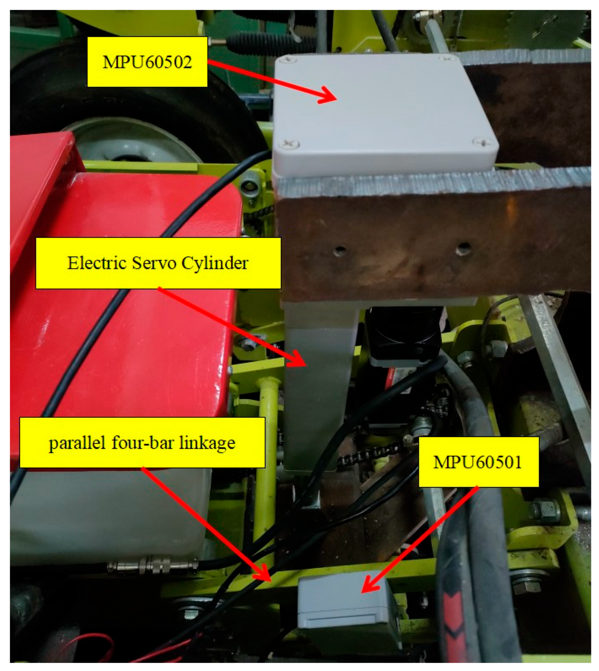
The experiment used an Electric Servo Cylinder produced by Dingying Intelligent to control the depth of broadcast. The Electric Servo Cylinder has a stroke of 150 mm, a ball screw lead of 5 mm, and a maximum speed of 50 mm/s. In order to conduct the long-term observation experiment, the speed of the travel electric cylinder was set to 0.01 mm/s. In the actual test, the travel speed of Electric Servo Cylinder did not have much influence on the sensor. This is because Electric Servo Cylinder travel mainly relies on the servo motor and ball screw drive. Compared to other motors and gear drives, the transmission torque is more stable and does not produce too much jitter. In order to ensure the accuracy of the experimental data, after the MCU sent the data reading command, we assessed whether the sensor was working normally by analyzing whether the number of bytes returned by the sensor was consistent with the regulations. A flashing red LED light means an alarm. An alarm will be triggered if the incorrect number of bytes is detected 10 times in a row.
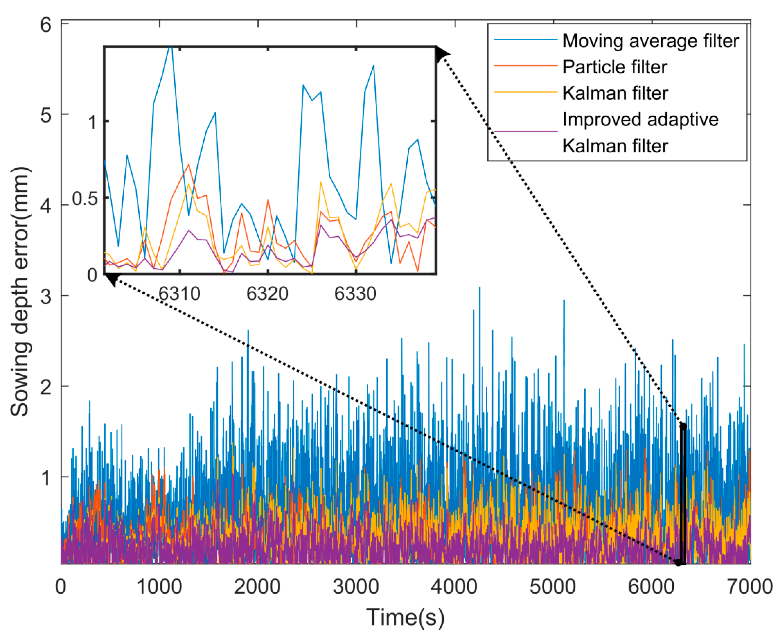
The experiment started from the position at which the sowing depth was 0 mm by controlling the Electric Servo Cylinder with the microcontroller. We set the Electric Servo Cylinder to extend downward at a constant speed from a predetermined speed. This allowed the sowing depth to vary until the predetermined depth of 7 cm was reached. At the same time, percussion vibration was artificially applied to the sowing monomer during the measurement. In the experiment, the sensor was disturbed by manually using a small hammer to knock on it, and the sowing monomer vibrated from bottom to top. The sowing depth was measured and calculated by the sensor. The experimental site for sowing the monomer is shown in Figure 13. The variation of the error of the experimental results is shown in Figure 14. The MSE of sowing depth measurement is shown in Table 2. It can be seen from the figure that the data acquisition error becomes larger when noise is artificially applied to the sowing monomer. This is mainly due to the impact the shock has on the accelerometer. It can be seen in the figure that the error curve represented by the MAF, PF, KF, and other algorithms increases with the changes in vibration and cannot be optimized with time, while the error curve of the IAKF algorithm has a large error in the initial state. However, over time, the adaptability to noise becomes stronger and the error lowers. It can be seen that the IAKF algorithm can still achieve a good accuracy in the actual scene and successfully improves the detection ability of the sowing depth.

5. Discussion and Conclusions

This paper mainly studied the method of sowing depth detection, the data filtering algorithm on the data acquisition of the attitude angle of the sowing monomer, and the rotation angle of the parallel four-bar linkage. By comparing the moving average filter algorithm, particle filter algorithm, Kalman filter algorithm, and improved adaptive Kalman filter algorithm using the MATLAB simulation, we found that the improved Kalman filter algorithm has better performance in noise adaptability, and in the improved Kalman filter algorithm with the extension of the filter time, MSE gradually becomes smaller and is closer to the true value, while the MSE of the remaining algorithms does not decrease significantly in the long run. This was also verified with physical testing. The improved adaptive Kalman filtering algorithm in this paper provides better detection accuracy for sowing depth detection. This study provides an important theoretical basis for the subsequent sowing depth control. This study can indirectly improve the accuracy of sowing depth control and increase the sowing depth qualification rate.
In this study, although the improved Kalman filter algorithm was used to obtain more accurate sowing depth data, the algorithm may still be affected by some environmental factors—such as air temperature, humidity, and soil hardness—in the field test. Therefore, in this paper, a field test was considered, and the detection system was further optimized by comparing the experimental measurement results with the theoretical values.

Author Contributions

Conceptualization, N.Z.; methodology, N.Z.; software, N.Z.; validation, N.Z. and S.Y.; formal analysis, N.Z.; investigation, N.Z.; resources, N.Z. and B.Z.; data curation, N.Z. and B.Z.; writing—original draft preparation, N.Z.; writing—review and editing, N.Z.; visualization, N.Z. and G.C.; supervision, N.Z. and Z.Z. All authors have read and agreed to the published version of the manuscript.

Funding

This research was financially supported by the National Youth Fund of China (NO. 32201655); the Major Science and Technology Special Projects of “Hundred, Thousand and Ten Thousand Talents Project” in Heilongjiang Province, China (NO.SC2020ZX17B0009).

Institutional Review Board Statement

Not applicable.

Informed Consent Statement

Not applicable.

Data Availability Statement

Not applicable.

Conflicts of Interest

The authors declare no conflict of interest.

References

  1. Gao, W.S. Development Trends and Basic Principles of Conservation Tillage. Sci. Agric. Sin. 2007, 40, 2702–2708. [Google Scholar]
  2. Sun, Z.Q.; Li, H.W.; Yang, L. 2BQM-2 Type Suction Precise Maize No-tillage Planter. J. Agric. Mech. Res. 2007, 2, 87–89. [Google Scholar]
  3. Yang, L.; Yan, B.X.; Zhang, D.X.; Zhang, D.X.; Zhang, T.L.; Wang, Y.X.; Cui, T. Research Progress on Precision Planting Technology of Maize. Trans. Chin. Soc. Agric. Mach. 2016, 47, 38–48. [Google Scholar]
  4. Zhou, S.H.; Wang, Z.H.; Huang, D.Y. No–Till Planter sowing Intelligent Depth Regulation System Based on Flex Sensor. J. Jilin Univ. 2020, 38, 555–562. [Google Scholar]
  5. Gao, Y.Y.; Wang, X.; Yang, S.; Zhai, C.Y.; Zhao, C.J. Development of CAN-based sowing Depth Monitoring and Evaluation System. Trans. Chin. Soc. Agric. Mach. 2019, 50, 23–32. [Google Scholar]
  6. Gao, Y.Y.; Zhai, C.Y.; Yang, S.; Zhao, X.G.; Wang, X.; Zhao, C.J. Development of CAN-based Downforce and sowing Depth Monitoring and Evaluation System for Precision Planter. Trans. Chin. Soc. Agric. Mach. 2020, 51, 15–28. [Google Scholar]
  7. Jiang, X.; Tong, J.; Ma, Y.; Li, J.; Wu, B.; Sun, J. Study of Tillage Depth Detecting Device Based on Kalman Filter and Fusion Algorithm. Nongye Jixie Xuebao/Trans. Chin. Soc. Agric. Mach. 2020, 51, 53–60. [Google Scholar]
  8. Suomi, P.; Oksanen, T. Automatic working depth control for seed drill using ISO 11783 remote control messages. Comput. Electron. Agric. 2015, 116, 30–35. [Google Scholar] [CrossRef]
  9. Ma, Y.C.; Zhang, W.; Li, Y.Q.; Che, G. Study on Two P rofiling M echanism of Planter Unit. J. Agric. Mech. Res. 2011, 33, 101–103, 106. [Google Scholar]
  10. Fitriani, D.A.; Kusuma, W.A.; Risqiwati, D. Design of monitoring system step walking with MPU6050 sensor based android. JOINCS 2016, 1, 1–8. [Google Scholar] [CrossRef]
  11. Liu, W.; Dai, J. Design of attitude sensor acquisition system based on STM32. In Proceedings of the 2015 Fifth International Conference on Instrumentation and Measurement, Computer, Communication and Control (IMCCC), Qinhuangdao, China, 18–20 September 2015; IEEE: Piscataway, NJ, USA, 2015; pp. 1850–1853. [Google Scholar]
  12. Jian, H. Design of angle detection system based on MPU6050. In Proceedings of the 7th International Conference on Education, Management, Information and Computer Science (ICEMC 2017), Shenyang, China, 16–18 June 2017; Atlantis Press: Paris, France, 2016; pp. 6–8. [Google Scholar]
  13. Ye, L. Azimuth Angle Algorithm Based on MPU6050 Sensor; Jilin University: Changchun, China, 2015. [Google Scholar]
  14. Hall, D.L.; Llinas, J. An introduction to multisensor data fusion. Proc. IEEE 1997, 85, 6–23. [Google Scholar] [CrossRef] [Green Version]
  15. Khaleghi, B.; Khamis, A.; Karray, F.O.; Razavi, S.N. Multisensor data fusion: A review of the state-of-the-art. Inf. Fusion 2013, 14, 28–44. [Google Scholar] [CrossRef]
  16. Wu, L. Study on Digital Filter Algorithms of Data Acquisition System; Beijing Forestry University: Beijing, China, 2015. [Google Scholar]
  17. Al-Mbaideen, A.A. Application of moving average filter for the quantitative analysis of the NIR spectra. J. Anal. Chem. 2019, 74, 686–692. [Google Scholar] [CrossRef]
  18. Gustafsson, F. Particle filter theory and practice with positioning applications. IEEE Aerosp. Electron. Syst. Mag. 2010, 25, 53–82. [Google Scholar] [CrossRef] [Green Version]
  19. Boers, Y.; Driessen, J.N. Particle filter based detection for tracking. In Proceedings of the 2001 American Control Conference (Cat. No. 01CH37148), Arlington, VA, USA, 25–27 June 2001; IEEE: Piscataway, NJ, USA, 2001; Volume 6, pp. 4393–4397. [Google Scholar]
  20. Hu, S.; Jing, Z. Overview of particle filter algorithm. Control. Decis. 2005, 20, 361–365, 371. [Google Scholar]
  21. Liang, J. Research on Particle Filter Algorithm and Its Application; Harbin Institute of Technology: Harbin, China, 2009. [Google Scholar]
  22. Meinhold, R.J.; Singpurwalla, N.D. Understanding the Kalman filter. Am. Stat. 1983, 37, 123–127. [Google Scholar]
  23. Di, W. Inertial Navigation Technology Based on Kalman Filtering; North China University of Technology: Beijing, China, 2018. [Google Scholar]
  24. Li, H.; Li, W.; Huang, Y. Multisensor measured data fusion based on Kalman filtering. Eng. J. Wuhan Univ. 2011, 44, 521–525. [Google Scholar]
  25. Li, Q.; Li, R.; Ji, K.; Dai, W. Kalman filter and its application. In Proceedings of the 2015 8th International Conference on Intelligent Networks and Intelligent Systems (ICINIS), Tianjin, China, 1–3 November 2015; IEEE: Piscataway, NJ, USA, 2015; pp. 74–77. [Google Scholar]
  26. Ge, J.; Dong, H.; Liu, H. Real-time Reduction of Magnetic Noise Associated with Ocean Waves via Sage Husa Algorithm for Towed Overhauser Marine Geomagnetic Sensor. Earth Sci. 2018, 43, 3792–3798. [Google Scholar]
  27. Zhou, D.H.; Xi, Y.G.; Zhang, Z.J. A suboptimal multipl fading extended kalman filter. Acta Autom. Sin. 1991, 17, 689–695. [Google Scholar]
  28. Narasimhappa, M.; Mahindrakar, A.D.; Guizilini, V.C.; Terra, M.H.; Sabat, S.L. MEMS-based IMU drift minimization: Sage Husa adaptive robust Kalman filtering. IEEE Sens. J. 2019, 20, 250–260. [Google Scholar] [CrossRef]
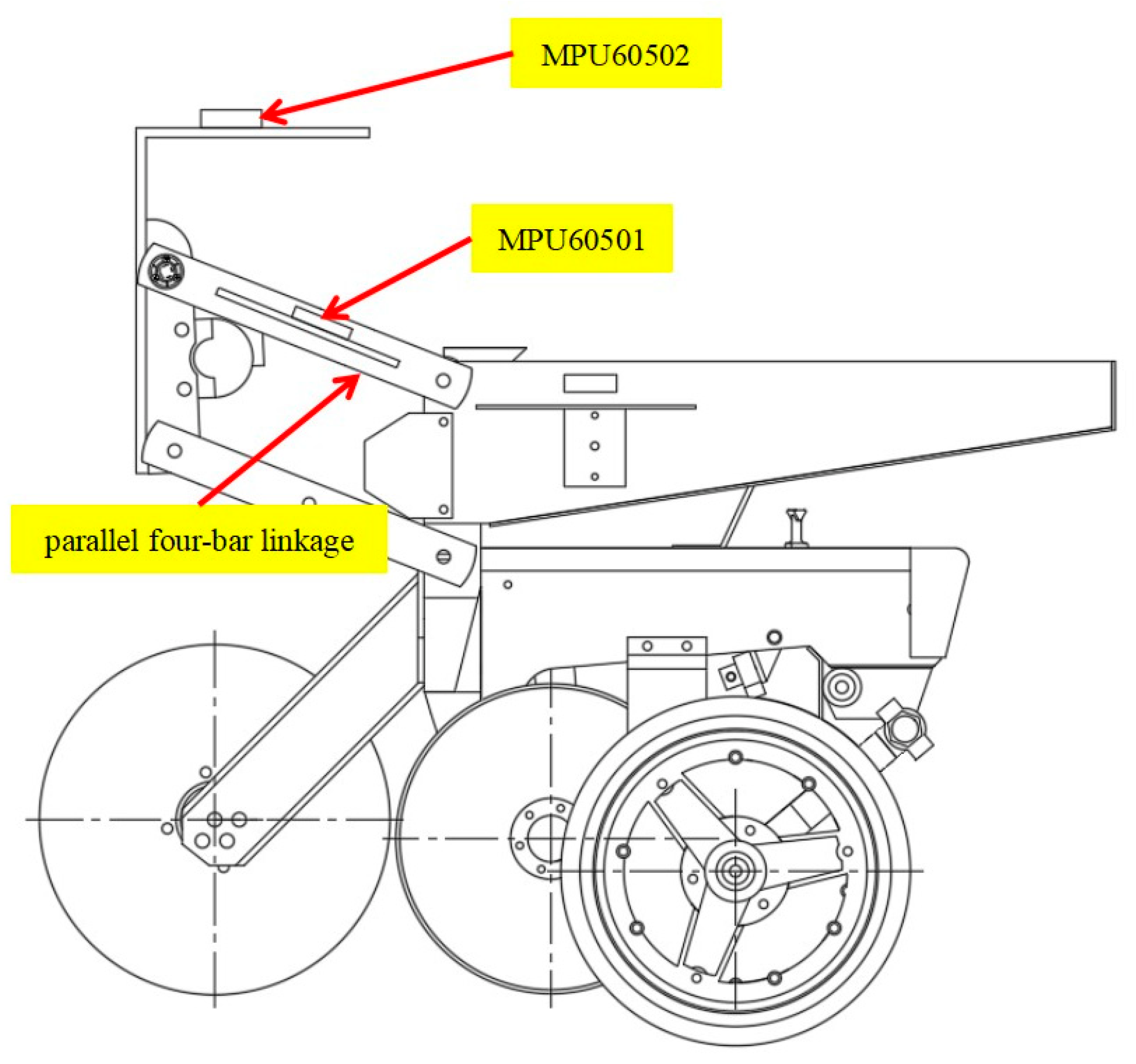
Figure 1. Two-dimensional structure diagram of the sowing monomer.
Electronics 11 03802 g001
Figure 2. Inclination detection diagram of the parallel four-bar linkage.
Electronics 11 03802 g002
Figure 3. Schematic diagram of the Kalman filtering algorithm.
Electronics 11 03802 g003
Figure 4. Parallel four-bar linkage rotation angle simulation.
Electronics 11 03802 g004
Figure 5. Parallel four-bar linkage rotation angle filtering error.
Electronics 11 03802 g005
Figure 6. Simulation of the attitude angle of the sowing monomer.
Electronics 11 03802 g006
Figure 7. Filtering error of the attitude angle of the sowing monomer.
Electronics 11 03802 g007
Figure 8. Principle of the adaptive Kalman filter algorithm.
Electronics 11 03802 g008
Figure 9. IAKF of the parallel four-bar linkage rotation angle simulation.
Electronics 11 03802 g009
Figure 10. IAKF of the parallel four-bar linkage rotation angle filtering error.
Electronics 11 03802 g010
Figure 11. Simulation of IAKF sowing monomer attitude angle.
Electronics 11 03802 g011
Figure 12. Filtering error of the IAKF sowing monomer attitude angle.
Electronics 11 03802 g012
Figure 13. Sowing monomer testing site.
Electronics 11 03802 g013
Figure 14. Error variation of the sowing monomer experiment.
Electronics 11 03802 g014
Table 1. Algorithm simulation of MSE.
Algorithm NameMSE
MPU60501MPU60502
Measure value0.42360.3037
MAF value0.14550.1047
PF value0.05170.0548
KF value0.04220.0404
Table 2. Sowing depth measurement MSE.
Algorithm NameSowing Depth MSE
Measure value1.8256
MAF value0.5968
PF value0.1807
KF value0.1449
IAKF value0.0636
Publisher’s Note: MDPI stays neutral with regard to jurisdictional claims in published maps and institutional affiliations.