Improved Linear Quadratic Regulator Lateral Path Tracking Approach Based on a Real-Time Updated Algorithm with Fuzzy Control and Cosine Similarity for Autonomous Vehicles

Abstract

Path tracking plays a crucial role in autonomous driving. In order to ensure the real-time performance of the controller and at the same time improve the stability and adaptability of the path tracking controller, a lateral path control strategy based on the improved LQR algorithm is proposed in this paper. To begin with, a discrete LQR controller with feedforward and feedback components is designed based on the error model of vehicle lateral dynamics constructed by the natural coordinate system. Then, a fuzzy control method is applied to adjust the weight coefficients of the LQR in real time according to the state of the vehicle. Furthermore, an update mechanism based on cosine similarity is designed to reduce the computational effort of the controller. The improved LQR controller is tested on a joint Simulink–Carsim simulation platform for a two-lane shift maneuver. The results show that the control algorithm improves tracking accuracy, steering stability and computational efficiency.

1. Introduction

Since Google, Baidu, Huawei, Tesla and other companies began to study autonomous driving technology, autonomous driving technology has ushered in a period of vigorous development in recent years [1]. Autonomous vehicles have been the subject of widespread debate worldwide due to the advantages of comfort, security and efficiency [2]. The automatic driving system includes environment perception and localization, decision making, path planning and path tracking [3]. Among these technologies, path tracking control is the core of intelligent driving, which is an important component to ensure vehicle driving safety, handling stability and other performances [4]. The study of path tracking control is of great importance in theoretical research and engineering applications, as it directly affects safety and user experience.

Path tracking is the process of executing a predefined path by controlling the steering and speed of the vehicle. The purpose of a path tracking controller is to reduce the lateral distance between the vehicle and the planned path, the difference between the vehicle’s heading and the expected path and the steering input to provide smooth motion while maintaining stability [5]. Different types of path tracking controllers have been designed in the last half-century. For example, the Pure pursuit and the Stanley method [6] are standard kinematics-based methodologies for autonomous vehicle path tracking. Although kinematic controllers can be designed without considering vehicle dynamics, they do not guarantee driving safety, especially in bad conditions. Therefore, there are many studies dedicated to path-tracking based on vehicle dynamics, such as traditional PID control, linear-quadratic regulators (LQR) [7], fuzzy logic control [8], sliding-mode control (SMC) [9] and model predictive control (MPC) [10].

As a traditional control method, the LQR control method has been used in a number of applications [11]. In 2009, Snider presented using the LQR control approach in path tracking, applying the vehicle centroid as the control point, modeling the system with path curvature disturbance and designing an LQR controller [12]. Although this control method can make the system more stable, it ignores the disturbances and generates systematic errors. As a result, NR Kapania proposed a feedforward steering controller with feedback [13]. This controller establishes a nonlinear vehicle dynamics model and presents a feedforward control component for the first time. The results show a decreasing trend of tracking bias at high-speed conditions. Xu et al. suggested adding a feedforward related to the path curvature to the LQR feedback control to reduce the steady-state deviation of the controller [14]. The LQR controller is an optimal control. It has the advantage that the controller ensures that the intelligent vehicle travels along the desired path while wasting the least amount of energy. The research-based LQR control method is widely used in smart vehicles, but there are input instability and computational problems in solving the LQR. This will affect the real-time performance and stability of the controller.

Intelligent control methods are based on the theory of advanced intelligent algorithms, the most common of which are fuzzy control, neural networks, genetic algorithms, etc. Applying intelligent control algorithms to the path tracking control of vehicles is the future trend [15,16]. Because fuzzy control uses human experience theory, it can simplify the complexity of the system and is an easy-to-control, robust nonlinear control method. Onieva [17] proposed an adaptive fuzzy controller which can update its membership functions and rule base in real time in an iterative genetic algorithm. Zhang [18] proposed a saturation-resistant output feedback controller based on T-S fuzzy control for nonlinear and unpredictable systems. Lian [19] built a fuzzy model-based system to represent a nonlinear networked vehicle system subject to hybrid cyberattacks for solving nonlinear autonomous vehicles that smoothly follow a planned path under perturbation. Yan [20] designed a fuzzy synchronous controller of a Takagi–Sugeno (T-S) fuzzy neural network with distributed time-varying delay and probabilistic network communication delay and applied it to image encryption. Yan [21] proposed a novel adaptive memory-event-triggered mechanism by studying the weighted memory-event-triggered $H_{\infty }$ static output control issue of uncertain Takagi–Sugano fuzzy wind power generation systems. Through data training, the neural network can mimic human learning behavior to improve the optimal control of the vehicle in various situations. H. Taghavifar [22] used neural network autoregression to accurately identify nonlinear vehicle dynamics to evaluate the system response. W. Zhang et al. used a two-layer deep reinforcement learning strategy to select the behavior with the highest payoff as the output of the neural network to deal with the overshoot problem during high-speed turns [23]. Although the combination of the path tracking controller and intelligent control algorithm has improved the tracking performance, the formulation of fuzzy control rules and the data training of neural networks are still tricky problems.

The above literature review outlines various research results on route tracking control strategies for autonomous vehicles and presents some of the problems faced by these approaches. Although LQR controllers can have full tracking accuracy during tracking maneuvers, the problem of driving comfort caused by fixed weights of the cost function when the vehicle is far from the desired path or driving in poor road conditions is less studied. Additionally, we investigate the trade-off between the sensitivity of the LQR controller to speed and the computational effort. The main contributions of this paper are as follows: (1) An LQR lateral path tracking controller including feedforward and feedback parts is designed, and the feedback coefficients are obtained by solving the cost function of the LQR controller by using the LaGrange multiplier method for the first time. (2) A calculation method is designed to calculate the coordinate information of the projection point of the real vehicle to the reference path according to the information of the nearest reference point on the path, which reduces the fluctuation of the controller input. (3) A strategy for the real-time updating of the LQR controller is formulated based on the fuzzy rules of lateral error and heading error. (4) An update rule based on cosine similarity is designed, which is used for the balance between the tracking accuracy and the calculation amount of the controller.

The rest of this paper is as follows: Section 2 presents the vehicle dynamics error model. In Section 3, we derive a detailed solution to the LQR lateral path tracking controller. Section 4 presents the improved LQR controller using fuzzy control and cosine similarity methods. Section 5 gives the simulation results under the Simulink–Carsim platform to evaluate the tracking performance of the improved LQR controller. Finally, we conclude the paper in Section 6.

2. Mathematical Model

2.1. Dynamics Model

Determining a reliable mathematical model is challenging because vehicle steering control systems have highly nonlinear and time-varying parameters. It is not easy to express the kinematic properties of the vehicle using only the kinematic model of the vehicle. Therefore, a simplified two-degree-of-freedom dynamics model will be used in this paper [24].

We assume that the car is symmetrical, while neglecting the distance between the wheels and combining the two wheels into one, which is the two-degree-of-freedom model dynamics model of the car. This dynamics model is shown in Figure 1.

Where ${\alpha }_f$ and ${\alpha }_r$ are the slip angles of the front and rear wheels. $a$ and $b$ indicate the distance from the front and rear axles to the center of mass. $v_f$ and $v_r$ denote the speed of the front and rear wheels. $F_{yf}$ and $F_{yr}$ are the lateral tire forces of the front and rear wheels. $\delta$ is the steering angle of the front wheel. Due to the sideslip angle of the center of mass, we can see that the speed direction of the wheel is not the same as the direction of the wheel. $v$ is the velocity at the center of mass, which generally does not coincide with the x-axis of the vehicle body coordinate system. By analyzing the momentum theorem in the y-axis direction of the car coordinate system and the momentum theorem at the center of mass, we can obtain:

$$\left\{\begin{array}{l}{\displaystyle \sum F_y}=m{a}_y=F_{yf}\cos \delta +F_{yr}\\ {\displaystyle \sum M=I_z\ddot{\phi }=a{F}_{yf}\cos \delta }-b{F}_{yr}\end{array}\right.$$

(1)

Considering that the steering angle $\delta$ is generally slight, we consider that $\cos \delta$ $\approx$ 1. Equation (1) can be simplified as:

$$\left\{\begin{array}{l}m{a}_y=F_{yr}+F_{yf}=C_{\alpha f}{\alpha }_f+C_{\alpha r}{\alpha }_r\\ I_z\ddot{\phi }=a{F}_{yf}-b{F}_{yr}=a{C}_{\alpha f}{\alpha }_f-b{C}_{\alpha r}{\alpha }_r\end{array}\right.$$

(2)

where $m$ is the mass of the whole vehicle. $I_z$ means the moment of inertia of the vehicle around the z-axis. $a_y$ represents the acceleration under the vehicle’s y-axis direction. $\phi$ is the yaw angle of a vehicle, which is the angle between the x-axis of the vehicle body and the X-axis of the inertial coordinate system. $\ddot{\phi }$ denotes the angular acceleration of the vehicle. $C_{\alpha f}$ and $C_{\alpha r}$ represent the linearized cornering stiffnesses of the front and rear wheels.

It is known from rigid body kinematics that the velocity of any point on a rigid body is equal to the combination of the velocity of the referenced point and the velocity around the referenced point. Figure 2 shows the combined relationship between the velocities of the front and rear wheels and the velocity of the center of mass in a two-degree-of-freedom model of the vehicle.

According to Figure 2, ${\alpha }_r$ can be expressed as follows:

$$\tan {\alpha }_r=\frac{\dot{\phi }b-v\sin \beta }{v\cos \beta }=\frac{\dot{\phi }b-v_y}{v_x}\approx {\alpha }_r$$

(3)

where $\beta$ represents the sideslip angle of the center of mass. $v_x$ and $v_y$ are the longitudinal speed and lateral speed of the car, respectively. Because ${\alpha }_r$ is a negative value in Figure 2, it can be rewritten as:

$$\frac{v_y-\dot{\phi }b}{v_x}\approx {\alpha }_r$$

(4)

By the same method, we can calculate ${\alpha }_f$ as:

$$\tan (\delta +{\alpha }_f)=\frac{\dot{\phi }a+v\sin \beta }{v\cos \beta }=\frac{\dot{\phi }a+v_y}{v_x}\approx \delta +{\alpha }_f$$

(5)

Since the lateral acceleration $a_y$ of the vehicle is related to the tangential and centripetal acceleration along the y-direction, it can be deduced as $a_y={\dot{v}}_y+v_x\dot{\phi }$. Assuming that the speed of the car is kept at a fixed value and applying Equations (3) and (5) to (2), the expression of the dynamics model of the vehicle is as follows:

$$\left[\begin{array}{c}{\dot{v}}_y\\ \ddot{\phi }\end{array}\right]=\left[\begin{array}{cc}\frac{C_{\alpha f}+C_{\alpha r}}{m{v}_x}& \frac{a{C}_{\alpha f}-b{C}_{\alpha r}}{m{v}_x}-v_x\\ \frac{a{C}_{\alpha f}-b{C}_{\alpha r}}{I_z{v}_x}& \frac{a^2{C}_{\alpha f}+b^2{C}_{\alpha r}}{I_z{v}_x}\end{array}\right]\left[\begin{array}{c}{v}_y\\ \dot{\phi }\end{array}\right]+\left[\begin{array}{c}-\frac{C_{\alpha f}}{m}\\ -\frac{a{C}_{\alpha f}}{I_z}\end{array}\right]\delta$$

(6)

2.2. Dynamics Tracking Error Model

To separate the horizontal and vertical control of the vehicle, we convert the dynamics model of the vehicle to a Frenet coordinate system. We use lateral and yaw errors as the state variables of the dynamics error model. This is because lateral and yaw errors occur when planning the vehicle’s path and current position when the intelligent vehicle is tracking its path in real-time. We need to design a controller to eliminate these two errors in real-time so that the vehicle can track our planned path quickly and accurately [25]

Figure 3 depicts the definition of the lateral error and yaw error. The lateral error is the distance between the projective point of the current vehicle position on the desired path and the current position, and the yaw error is the deviation between the yaw angle of the current position and the tangent orientation of the projective point on the desired path. Where $\dot{s}$ is the velocity of the projective point. $\theta$ and ${\theta }_r$ are the heading angles of the velocity at the current position and the projective point, respectively, and the $r$ in the lower right corner means the reference. From Figure 3, the expression of $e_d$ can be obtained as follows:

$$e_d=\left(\overrightarrow{r}-{\overrightarrow{r}}_r\right)•{\overrightarrow{n}}_r$$

(7)

Equation (7) is a vector dot product, and the result is a scalar. By taking the derivative on both sides of the expression of the lateral error, we can calculate the expression of the lateral error rate as:

$${\dot{e}}_d=\left(\dot{\overrightarrow{r}}-{\dot{\overrightarrow{r}}}_r\right)•{\overrightarrow{n}}_r+\left(\overrightarrow{r}-{\overrightarrow{r}}_r\right)•{\dot{\overrightarrow{n}}}_r$$

(8)

According to the vector derivation rule, we can obtain the expression of ${\dot{e}}_d$:

$${\dot{e}}_d=v\overrightarrow{\tau }•{\overrightarrow{n}}_r$$

(9)

Because the angle between $\overrightarrow{\tau }$ and ${\overrightarrow{n}}_r$ is $\pi /2-(\theta -{\theta }_r)$, and both are vectors, the expression of ${\dot{e}}_d$ can be rewritten as:

$${\dot{e}}_d=v\left|\overrightarrow{\tau }\right|\left|{\overrightarrow{n}}_r\right|\cos 〈\overrightarrow{\tau },{\overrightarrow{n}}_r〉=v\sin (\theta -{\theta }_r)$$

(10)

From Figure 1, the heading angle $\theta$ is the sum of $\phi$ and $\beta$. It can be deduced that $v_x=v\cos \beta$ and $v_y=v\sin \beta$. At the same time, we define $e_{\phi }=\phi -{\theta }_r$. Because the difference between the values of $\phi$ and ${\theta }_r$ is minimal, ${\dot{e}}_d$ can be simplified as:

$${\dot{e}}_d=v_x{e}_{\phi }+v_y$$

(11)

Because the reference heading angle is relatively smooth when designing the path, we ignore the higher-order derivative of ${\theta }_r$. In addition, when designing the lateral motion controller, we do not consider the effect of longitudinal velocity and let $v_x$ be a constant value. This gives us the conversion equations from the dynamics model to the dynamics error model:

$$\left\{\begin{array}{l}{v}_y={\dot{e}}_d-v_x{e}_{\phi }\\ {\dot{v}}_y={\ddot{e}}_d-v_x{\dot{e}}_{\phi }\\ \dot{\phi }={\dot{e}}_{\phi }+{\dot{\theta }}_r\\ \ddot{\phi }={\ddot{e}}_{\phi }\end{array}\right.$$

(12)

Equation (18) is applied to (7), and the simplified arrangement can be obtained:

$${\ddot{e}}_{\mathrm{d}}=\left(\frac{C_{\alpha \mathrm{f}}+C_{\alpha \mathrm{r}}}{m{v}_{\mathrm{x}}}\right){\dot{e}}_{\mathrm{d}}+\left(-\frac{a{C}_{\alpha \mathrm{f}}-b{C}_{\alpha \mathrm{r}}}{m}\right)e_{\phi }+\left(\frac{a{C}_{\alpha \mathrm{f}}-b{C}_{\alpha \mathrm{r}}}{m{v}_{\mathrm{x}}}\right){\dot{e}}_{\phi }+\left(\frac{a{C}_{\alpha \mathrm{f}}-b{C}_{\alpha \mathrm{r}}}{m{v}_{\mathrm{x}}}\right){\dot{\theta }}_{\mathrm{r}}+\left(-\frac{C_{\alpha \mathrm{f}}}{m}\right)\delta$$

(13)

$${\ddot{e}}_{\phi }=\left(\frac{a{C}_{\alpha \mathrm{f}}-b{C}_{\alpha \mathrm{r}}}{I_z{v}_{\mathrm{x}}}\right){\dot{e}}_{\mathrm{d}}+\left(-\frac{a{C}_{\alpha \mathrm{f}}-b{C}_{\alpha \mathrm{r}}}{I_z}\right)e_{\phi }+\left(\frac{a^2{C}_{\alpha \mathrm{f}}+b^2{C}_{\alpha \mathrm{r}}}{I_z{v}_{\mathrm{x}}}\right){\dot{e}}_{\phi }+\left(\frac{a^2{C}_{\alpha \mathrm{f}}+b^2{C}_{\alpha \mathrm{r}}}{I_z{v}_{\mathrm{x}}}\right){\dot{\theta }}_{\mathrm{r}}+\left(-\frac{a{C}_{\alpha \mathrm{f}}}{I_z}\right)\delta$$

(14)

The lateral error, lateral error rate, yaw error and yaw error rate are selected as new state variables. Moreover, the steering angle $\delta$ is employed as the input. The state-space of the dynamics error model can be expressed as:

$$\begin{array}{l}\left[\begin{array}{c}{\dot{e}}_d\\ {\ddot{e}}_d\\ {\dot{e}}_{\phi }\\ {\ddot{e}}_{\phi }\end{array}\right]=\left(\begin{array}{cccc}0& 1& 0& 0\\ 0& \frac{C_{\alpha f}+C_{\alpha r}}{m{v}_x}& -\frac{C_{\alpha f}+C_{\alpha r}}{m}& \frac{a{C}_{\alpha f}-b{C}_{\alpha r}}{m{v}_x}\\ 0& 0& 0& 1\\ 0& \frac{a{C}_{\alpha f}-b{C}_{\alpha r}}{I_z{v}_x}& -\frac{a{C}_{\alpha f}-b{C}_{\alpha r}}{I_z}& \frac{a^2{C}_{\alpha f}+b^2{C}_{\alpha r}}{I_z{v}_x}\end{array}\right)\left(\begin{array}{c}{e}_d\\ {\dot{e}}_d\\ e_{\phi }\\ {\dot{e}}_{\phi }\end{array}\right)+\left(\begin{array}{c}0\\ -\frac{C_{\alpha f}}{m}\\ 0\\ -\frac{a{C}_{\alpha f}}{I_z}\end{array}\right)\delta \\ \hspace{1em}\hspace{1em}\hspace{1em}+\left(\begin{array}{c}0\\ \frac{a{C}_{\alpha f}-b{C}_{\alpha r}}{m{v}_x}-v_x\\ 0\\ \frac{a^2{C}_{\alpha f}+b^2{C}_{\alpha r}}{I_z{v}_x}\end{array}\right){\dot{\theta }}_r\end{array}$$

(15)

The dynamics error model of the vehicle can be further simplified as

$$\dot{E}=AE+Bu+C{\dot{\theta }}_r$$

(16)

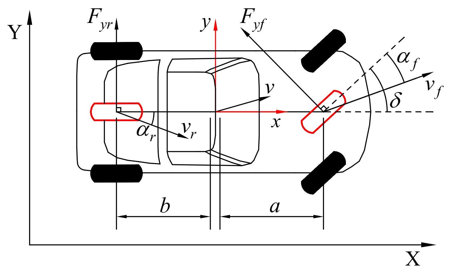
3. Lateral Control System Design

Based on the dynamics error model of the vehicle, we design the LQR controller shown in Figure 4 to achieve the lateral control of the vehicle and the fast convergence of the lateral error and yaw error so that the vehicle can better track on the desired path.

First, a dynamics error model is developed based on the parameters of the vehicle. Based on this mathematical model, we design the discrete LQR controller and obtain the feedback coefficients. Then, the current vehicle position is obtained by the environment sensing system, and the state variables between the vehicle and the desired path are calculated. Second, the feedforward module calculates the desired heading angular rate compensation from the feedback coefficients and the projection point information, which is neglected in the LQR module. Finally, the feedback coefficients calculated by the LQR controller, the current position information and the feedforward part are input to the vehicle controller to control the front wheel angle of the vehicle to drive the vehicle on the desired path.

3.1. LQR Controller Design

LQR control is an optimal control used to solve the stability problem of a system with minimum cost, which has been used in many control systems such as aircraft control, inverted pendulum control systems, automatic operation, etc. According to the dynamics error model of the vehicle, the input is the front wheel steering angle, and the state variables are the lateral error and yaw error and their first-order derivatives, respectively. Our control objective is to select the appropriate input $u$ so that the lateral and yaw errors are as small as possible. We can solve this problem with the LQR control algorithm.

The linear quadratic regulator is studied for linear systems in the form of state-space equations in modern control theory, where the cost function is a quadratic form function of state variables and control inputs. The advantage of LQR in intelligent driving lateral control is that when the system state deviates from the steady state due to obstacles or unexpected events, it ensures that the intelligent vehicle tracking control system approaches the ideal path without causing too much computational effort. The LQR control problem of a vehicle lateral path tracking controller can be expressed as:

$$\left\{\begin{array}{l}\min J={\displaystyle \sum _{k=0}^{\infty }\left(E_k^{T}Q{E}_k+u_k^{T}R{u}_k\right)}\\ s.t :\dot{E}=AE+Bu\end{array}\right.$$

(17)

where $Q=diag\left[q_1,q_2,q_3,q_4\right]$, $q_1$, $q_2$, $q_3$ and $q_4$ represent the weight coefficient of the lateral error, lateral error rate, yaw error and yaw error rate, respectively. $R=[r]$, where $r$ denotes the weight coefficient of the steering angle of the front wheels. The weight coefficient indicates the level of importance to this variable. The larger the value, the faster the corresponding state variables will converge.

Because in practical applications, especially on computers, we deal with discrete data, and in path planning we often plan a series of reference points rather than a continuous path, we choose to use discrete LQR control. To design the discrete LQR controller, we first ignore the $C{\dot{\theta }}_r$ in the dynamics error model, discretize Equation (16) and integrate both sides of the equation separately. It can be determined that:

$${\displaystyle {\int }_t^{t+dt}\dot{E}}dt={\displaystyle {\int }_t^{t+dt}(AE+Bu)}dt$$

(18)

where $dt$ is the sampling period of discrete control. According to the mean value theorem of definite integrals, we can obtain:

$$\left\{\begin{array}{l}E(t+dt)-E(t)=AE(\xi )dt+\mathrm{Bu}(\xi )dt\\ s.t :\xi \in (t,t+dt)\end{array}\right.$$

(19)

Usually, the accuracy of the midpoint Euler method is higher, but because the input only knows the input of the current period, the mixed-use of the forward Euler method and the midpoint Euler method is adopted. We define $E(\xi )=(E(t)+E(t+dt))/2$ and $u(\xi )=u(t)$ and apply it to Equation (19), resulting in:

$$E(t+dt)={\left(I-\frac{Adt}{2}\right)}^{-1}\left(I+\frac{Adt}{2}\right)E(t)+{\left(I-\frac{Adt}{2}\right)}^{-1}Bdtu(t)$$

(20)

where $I$ means the identity matrix. Let $\overline{A}={(I-Adt/2)}^{-1}(I+Adt/2)$ and $\overline{B}={(I-Adt/2)}^{-1}Bdt$. Equation (20) can be rewritten as

$$E(k+1)=\overline{A}E(k)+\overline{B}u(k)$$

(21)

Equation (21) is the discrete dynamics error model. Because the infinity in Equation (17) is challenging to deal with, it can be rewritten as:

$$\left\{\begin{array}{l}J={\displaystyle \sum _{k=0}^{n-1}\left(E_k^{T}Q{E}_k+u_k^{T}R{u}_k\right)}+E_n^{T}Q{E}_n n\to \infty \\ s.t :E(k+1)=\overline{A}E(k)+\overline{B}u(k)\end{array}\right.$$

(22)

Then, the LaGrange multiplier method is used to construct the unconstrained optimization problem to solve the extrema. The cost function with constraints is as follows:

$$J={\displaystyle \sum _{k=0}^{n-1}\left(E_k^{T}Q{E}_k+u_k^{T}R{u}_k\right)}+E_n^{T}Q{E}_n+{\displaystyle \sum _{k=0}^{n-1}{\lambda }_{k+1}^T}\left(\overline{A}{E}_k+\overline{B}{u}_k-E_{k+1}\right)$$

(23)

By constructing the Hamiltonian function, $H_k=E_k^{T}Q{E}_k+u_k^{T}R{u}_k+{\lambda }_{k+1}^T\left(\overline{A}{E}_k+\overline{B}{E}_k\right)$, and taking it into Equation (23), the cost function can be simplified as:

$$J={\displaystyle \sum _{k=0}^{n-1}\left(H_k-{\lambda }_k^T{E}_k\right)}+E_n^{T}Q{E}_n-{\lambda }_n^T{E}_n+{\lambda }_0^T{E}_0$$

(24)

Then, take the derivative of each item to make them equal to zero. Using the knowledge of vector derivatives, we can obtain the following equation:

$$\left\{\begin{array}{l}\frac{\partial J}{\partial E_k}=\overrightarrow{0}\Rightarrow {\lambda }_k=2Q{E}_k+{\overline{A}}^T{\lambda }_{k+1}(k=1,2,3\cdots n-1)\\ \frac{\partial J}{\partial u_k}=\overrightarrow{0}\Rightarrow u_k=-\frac{1}{2}{R}^{-1}{\overline{B}}^T{\lambda }_{k+1}(k=1,2,3\cdots n-1)\\ \frac{\partial J}{\partial {\lambda }_k}=\overrightarrow{0}\Rightarrow E_{k+1}=\overline{A}{E}_k+\overline{B}{u}_k(k=1,2,3\cdots n-1)\\ \frac{\partial J}{\partial E_n}=\overrightarrow{0}\Rightarrow {\lambda }_n=2Q{E}_n\end{array}\right.$$

(25)

By solving Equation (25), we can figure out:

$${\lambda }_{n-1}=2\left(Q+{\overline{A}}^{T}Q{\left(I+\overline{B}{R}^{-1}{\overline{B}}^{T}Q\right)}^{-1}\overline{A}\right)E_{n-1}$$

(26)

Equation (26) and ${\lambda }_n=2Q{E}_n$ have similar forms. When we start recurring from $n$, we can obtain the expression of ${\lambda }_{n-1}$ and ${\lambda }_{n-2}$ until ${\lambda }_1$. If we define ${\lambda }_k=2P_k{E}_k$, where $P_k=Q$, the value of $P_{k-1}$ can be inferred:

$$P_{k-1}=Q+{\overline{A}}^T{P}_k{\left(I+\overline{B}{R}^{-1}{\overline{B}}^T{P}_k\right)}^{-1}\overline{A}$$

(27)

Equation (27) is known as the Riccati equation. When the value of $P$ is iterated many times, the value of $P$ will converge. By calculating the Riccati equation, we can obtain the control quantity of the LQR controller as follows:

$$u_k=-{\left(R+{\overline{B}}^{T}P\overline{B}\right)}^{-1}{\overline{B}}^{T}P\overline{A}{E}_k$$

(28)

Equation (28) can be simplified as:

$$u_k=-k{E}_k$$

(29)

where $k=\left[k_1,k_2,k_3,k_4\right]$ is the outcome of the LQR controller and the feedback coefficient of the steering angle of the front wheels.

3.2. Feedforward Controller Design

Through applying Equation (29) to (16), the following equation is obtained:

$$\dot{E}=(A-Bk)E+C{\dot{\theta }}_r$$

(30)

If $\dot{E}$ is equal to 0, the equilibrium point of the state variables is not equal to 0. In other words, the vehicle’s lateral error and yaw error are not guaranteed to be 0. The LQR controller contains only a feedback part, which is not sufficient for our control needs. We need to design the feedforward part to eliminate the effect of $C{\dot{\theta }}_r$. The solution is to introduce a feedforward control ${\delta }_f$. The steering angle can be expressed as:

$$u=-kE+{\delta }_f$$

(31)

Similarly, if $\dot{E}$ is equal to 0, the expression of the state variables can be obtained:

$$E=-{(A-Bk)}^{-1}A\left(B{\delta }_f+C{\dot{\theta }}_r\right)$$

(32)

where all expressions in Equation (38) are known. With the help of the computer software, it can be determined that:

$$\left[\begin{array}{c}{e}_d\\ {\dot{e}}_d\\ e_{\phi }\\ {\dot{e}}_{\phi }\end{array}\right]=\left[\begin{array}{c}\frac{1}{k_1}\left\{{\delta }_f-\frac{{\dot{\theta }}_r}{v_x}\left[a+b-b{k}_3-\frac{m{v}_x^2}{a+b}\left(\frac{b}{C_{\alpha f}}+\frac{a}{C_{\alpha r}}{k}_3-\frac{a}{C_{\alpha r}}\right)\right]\right\}\\ 0\\ -\frac{{\dot{\theta }}_r}{v_x}\left(b+\frac{a}{a+b}\frac{m{v}_x^2}{C_{\alpha r}}\right)\\ 0\end{array}\right]$$

(33)

Obviously, the lateral error can make the steady-state error 0 through the feedforward part ${\delta }_f$. Nevertheless, the steady-state error of the yaw error will not be affected by ${\delta }_f$.

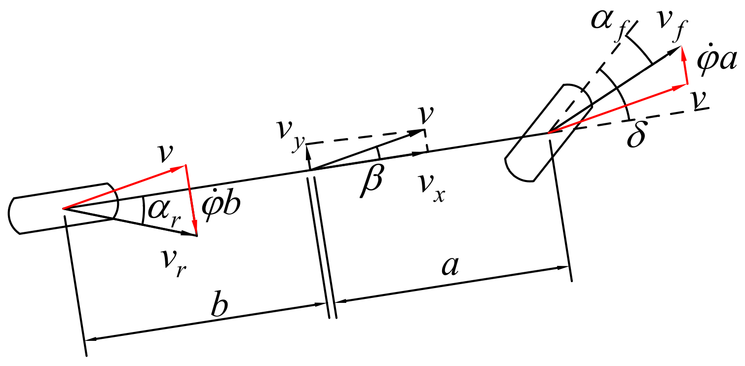
From Figure 3, the following equation can be obtained:

$${\overrightarrow{r}}_r+e_d{\overrightarrow{n}}_r=\overrightarrow{r}$$

(34)

By deriving from both sides of Equation (34) and substituting it with Equations (4), (5), (8) and (10), the following equation can be obtained:

$$\dot{s}{\overrightarrow{\tau }}_r+v\sin (\theta -{\theta }_r){\overrightarrow{n}}_r+e_d(-k\dot{s}\overrightarrow{\tau })=v\overrightarrow{\tau }$$

(35)

By multiplying both sides of Equation (35) by ${\overrightarrow{\tau }}_r$, we calculate $\dot{s}$ as:

$$\dot{s}=\frac{v_x\cos \left(\phi -{\theta }_r\right)-v_y\sin \left(\phi -{\theta }_r\right)}{1-K{e}_d}$$

(36)

In order to guarantee the smoothness of the vehicle, the planned driving route is a smooth curve, so the curvature $\left|K\right|$ of the path is much smaller than one. Therefore, when the vehicle is traveling along this path, the error $\left|e_{\phi }\right|$ between the actual yaw angle of the vehicle and the yaw angle on the desired path is also much smaller than one. Considering that there is no drift during the driving process of the vehicle, the lateral speed $\left|v_y\right|$ is far less than one. When $\left|K\right|\ll 1$, $\left|e_{\phi }\right|\ll 1$ and $\left|v_y\right|\ll 1$, we can obtain $\dot{s}\approx v_x$. According to the definition of the curvature, we can know that $K={\dot{\theta }}_r/\dot{s}$. Moreover, because $a_y\approx v_x^2/R$, the steady-state error of the yaw error can be expressed as:

$$e_{\phi }=\left(\frac{b}{R}+\frac{a}{a+b}m{a}_y\frac{1}{C_r}\right)$$

(37)

Moreover, because the vehicle is assumed to be rigid, according to the equivalent substitution method, the final form of $e_{\phi }$ is:

$$e_{\phi }=-\left(\frac{b}{R}+{\alpha }_r\right)$$

(38)

In Figure 5, $O$ is the center of the vehicle’s steering circle. The turning radius of the rear axle and the turning radius of the center of mass are approximately equal to form an isosceles triangle, approximately. Because the angle γ is a small value, it can be expressed as $\gamma \approx b/R$. According to the interior angle of the triangle, the sideslip angle $\beta$ can be calculated as:

$$-\beta =-\left(\frac{b}{R}+{\alpha }_r\right)$$

(39)

From Equations (38) and (39), we can obtain the conclusion $e_{\phi }=-\beta$. Due to $\theta =\phi +\beta$, the steady-state error of the yaw error does not need feedforward control to eliminate. The feedforward part is:

$${\delta }_f=\frac{v_x\cos \left(\phi -{\theta }_r\right)-v_y\sin \left(\phi -{\theta }_r\right)}{1-K{e}_d}\frac{K}{v_x}\left[a+b-b{k}_3-\frac{m{v}_x^2}{a+b}\left(\frac{b}{C_{\alpha f}}+\frac{a}{C_{\alpha r}}{k}_3-\frac{a}{C_{\alpha r}}\right)\right]$$

(40)

3.3. Predictive Controller Design

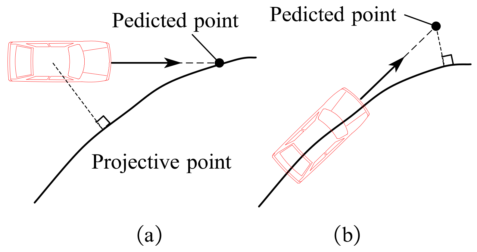
In the process of human driving, the human operation often has a certain predictability, which determines the human driving decision. As shown in the scenario in Figure 6, in (a), there is an error between the current position and the desired path, but when driving with the current situation, the vehicle will drive on the desired path, so the human will not change the driving behavior at this time, but the algorithm will move closer to the desired path to reduce the error. In (b), the current position of the vehicle is on the desired path, but when the vehicle continues to drive with the current state, the vehicle will deviate from the desired path, and the algorithm will not take action, but the human will change the steering wheel turning angle while driving.

The lagging nature of vehicle controllers and sensors makes it impossible to ensure good real-time performance, so predicting the vehicle’s travel path is essential. The prediction module is used to predict the future path of the vehicle to ensure that the vehicle travels on the desired path. Definition $t_p$ is the prediction time. It is assumed that the speed and angular velocity of the vehicle remain constant over the predicted time range. According to the kinematic models $\dot{x}=v\cos (\theta )$ and $\dot{y}=v\sin (\theta )$, by integration, we can obtain:

$$\left\{\begin{array}{l}{x}_{pre}=x_0+{\displaystyle \underset{0}{\overset{t_p}{\int }}[v_x\cos \phi (t)-v_y\sin \phi (t)]dt}\\ y_{pre}=y_0+{\displaystyle \underset{0}{\overset{t_p}{\int }}[v_y\cos \phi (t)+v_x\sin \phi (t)]dt}\end{array}\right.$$

(41)

where $x_0$ and $y_0$ represent the location information of the vehicle in the current time. $x_{pre}$ and $y_{pre}$ represent the predicted position information of the vehicle. $\phi (\tau )={\phi }_0+\dot{\phi }\tau$, where ${\phi }_0$ is the yaw angle of the current moment. By calculating Equation (41), the predicted location information can be obtained as follows:

$$\left\{\begin{array}{l}{x}_{pre}=x_0+\frac{v_x}{\dot{\phi }}\left(\sin ({\phi }_0+\dot{\phi }{t}_p)-\sin ({\phi }_0)\right)+\frac{v_y}{\dot{\phi }}\left(\cos ({\phi }_0+\dot{\phi }{t}_p)-\cos ({\phi }_0)\right)\\ y_{pre}=y_0+\frac{v_y}{\dot{\phi }}\left(\sin ({\phi }_0+\dot{\phi }{t}_p)-\sin ({\phi }_0)\right)-\frac{v_x}{\dot{\phi }}\left(\cos ({\phi }_0+\dot{\phi }{t}_p)-\cos ({\phi }_0)\right)\\ {\phi }_{pre}={\phi }_0+\dot{\phi }{t}_p\end{array}\right.$$

(42)

4. Improved Method of the LQR Controller

The LQR controller needs to track the desired path quickly and accurately under different path conditions and emergency situations. Weighting factors play an important role in the performance of the LQR controller, but the choice of weighting factors usually depends on human experience. To better compare the effect of each weighting factor on path tracking, we performed simulations using Simulink and Carsim software, setting the state variables and input weighting factors to 1. The desired path is a double-lane change path. Figure 7 and Figure 8 depict the results of the LQR controller with different weight factors. From the figures, it can be seen that the vehicle tracking performance is better when the weight coefficients are all 1.

In the figure, the variation in the $q_1$ and $q_4$ lateral and yaw error rates corresponding to the weight coefficients affects the vehicle path tracking control performance. When $q_1$ and $q_4$ are too large or too small, the vehicle cannot quickly eliminate the error and stay on the desired path. However, $q_2$, $q_3$ and $r$ have little effect on path tracking.

In addition, the input of the controller also has an effect on the vehicle, and the effect of different $r$ values on the steering angle of the front wheels is shown in Figure 9. When $r$ is small, the fluctuation of the steering angle is drastic, while when $r$ is larger, there will still be some fluctuation, although it can effectively reduce the fluctuation of the steering angle. The frequent fluctuation of the input signal is not good for the control of the vehicle and will also affect the service life of the vehicle.

Because the simulation is carried out in the simulation environment on the computer, the LQR controller updates the state matrix of the controller with the latest vehicle lateral speed $v_x$ in each running cycle to calculate the feedback coefficient $k$. Although it improves the tracking performance of the controller, it will cause the program to run slowly and put much pressure on the computer. The actual driving environment is terrible, which requires the controller to have a good real-time performance, so this approach cannot be applied well to the actual driving situation.

When the output feedback coefficient $k$ of the LQR controller is calculated according to a fixed $v_x$, then use the calculated $k$ to control the vehicle. Figure 10 shows the effect of path tracking at different longitudinal speeds. Obviously, when the established dynamics model is quite different from the actual longitudinal velocity, the tracking performance of the LQR controller will become very poor. This proves that the LQR controller has a high sensitivity to the longitudinal velocity $v_x$.

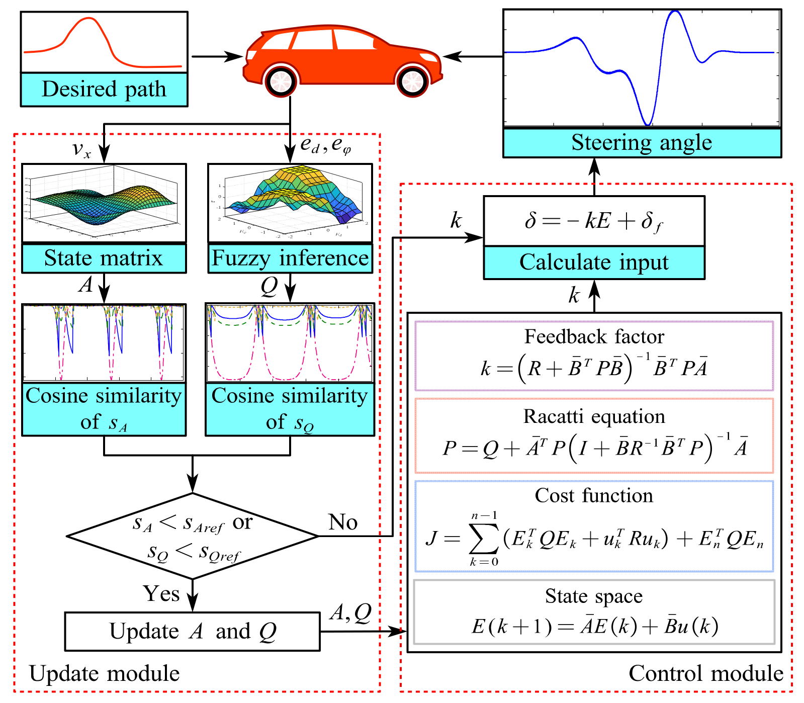
In order to improve the stability and real-time performance of the LQR controller, we propose an improved LQR path tracking strategy. The specific implementation process is shown in Figure 11, and the control strategy is mainly divided into two parts. First, the control module uses the LQR algorithm to calculate the steering angle according to the vehicle dynamics error model. Second, the update module calculates the cosine similarity between the real-time state matrix and the weight coefficient matrix obtained by fuzzy inference and the state matrix and weight coefficient matrix of the controller. Once one of the cosine similarities falls below the set update threshold, the updated state matrix and weight coefficient matrix will replace the state matrix and weight coefficient matrix of the control module. Then, the calculation process of LQR control is repeated, and the new feedback coefficients are obtained. If the cosine similarity is larger than the update threshold, it is not recalculated, and the previous feedback coefficient $k$ is used.

4.1. New Method for Calculating Projective Points

In the previous article, we mentioned that the error is calculated based on the current position of the vehicle and its projection point on the desired path. However, when the planned path is a closed curve, there will be more than one projection point, and it is not easy to find the projection point for continuous curves.

In practical planning paths, we often use discrete points to form the planning path. In addition, the error is calculated by using the point closest to the current position of the vehicle as the projection point. Although this does not cause much error compared to the data of the actual projection point, the fluctuation of the front wheel steering angle shown in Figure 9 may be caused by the inaccurate error calculation. When the vehicle switches from one reference point to the next, the reference point information changes abruptly, which leads to a sudden change in the error calculation results. According to $u=-kE+{\delta }_f$, the sudden change in the error will directly affect the front wheel steering angle of the vehicle, thus causing the fluctuation of the steering angle. For this phenomenon, the impact can be reduced by increasing the number of planning points. However, it is not feasible to increase the number of planning points, which will bring huge computation and affect the real-time performance of path tracking.

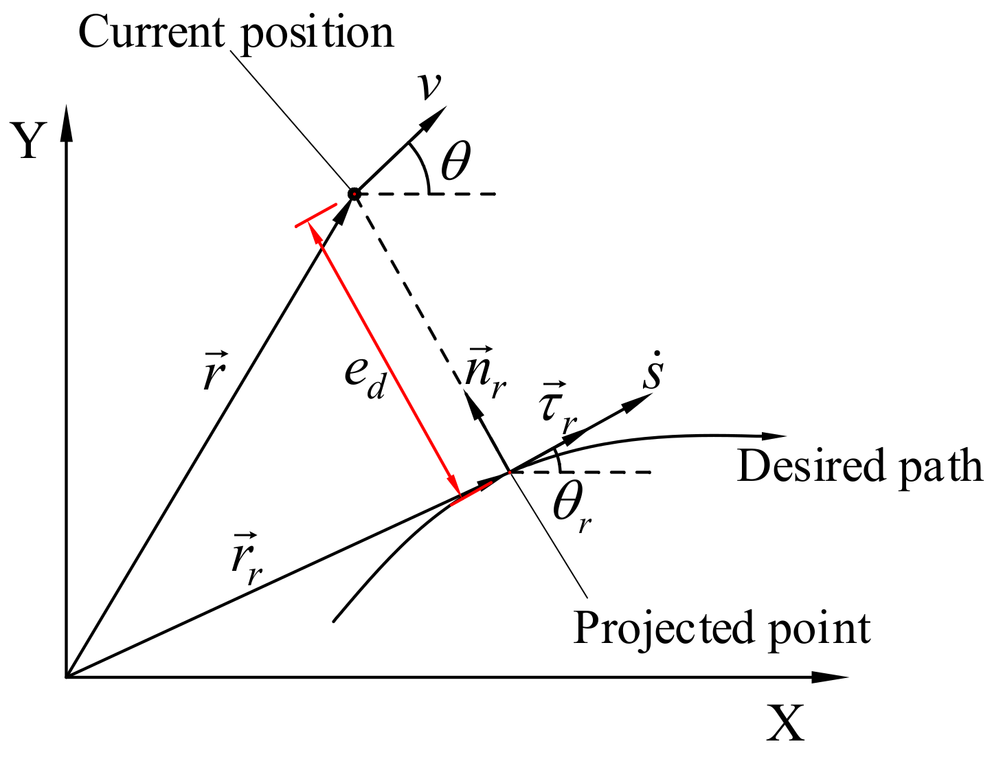
For the above case, we propose an improved method which can accurately estimate the information of the actual projected points at the current location without increasing the density of planning points. In Figure 12, the red dots represent the actual projected points, the black dots represent the current position of the vehicle and the blue dots represent the discrete trajectory points. ${\overrightarrow{\tau }}_m$ and ${\overrightarrow{n}}_m$ are the tangential unit direction and normal unit direction of the planning point closest to the current location.

It is not difficult to see from Figure 12 that the lateral error between the current position and the actual projective point can be expressed as:

$$e_d\approx (\overrightarrow{r}-{\overrightarrow{r}}_r)•{\overrightarrow{n}}_m$$

(43)

The arc length between the matching point and the projective point can be approximately expressed by $e_s$, and it can be approximated as follows:

$$e_s\approx (\overrightarrow{r}-{\overrightarrow{r}}_r)•{\overrightarrow{\tau }}_m$$

(44)

Especially in the straight-line segment, Equation (43) can accurately express the value of the lateral error. Because the matching point is close to the projection point and the curvature of the path is relatively stable when planning the path, there will not be much of a sudden change. We assume that the curvature between the matching point and the projection point is the same, and the trajectory between the matching point and the projection point can be approximated as an arc. Figure 13 shows this relationship between the projection and matching point

According to Equation (44), we can calculate ${\theta }_r$ as:

$${\theta }_r={\theta }_m+K_m{e}_s$$

(45)

By combining Equations (10), (36), (43), (44) and (45), the state error of the projective point is expressed as:

$$\left\{\begin{array}{l}{K}_r=K_m\\ {\theta }_r={\theta }_m+K_r(\overrightarrow{r}-{\overrightarrow{r}}_r)•{\overrightarrow{\tau }}_m\\ e_d=(\overrightarrow{r}-{\overrightarrow{r}}_r)•{\overrightarrow{n}}_m\\ e_{\phi }=\phi -{\theta }_r\\ {\dot{e}}_d=v_x\sin (\phi -{\theta }_r)+v_y\cos (\phi -{\theta }_r)\\ {\dot{e}}_{\phi }=\dot{\phi }-K_r\frac{v_x\cos \left(\phi -{\theta }_r\right)-v_y\sin \left(\phi -{\theta }_r\right)}{1-K_r{e}_d}\end{array}\right.$$

(46)

4.2. Update of the Weight Coefficient Based on Fuzzy Control

Fuzzy control algorithms are characterized by the fact that they do not require accurate modeling of the control system and are highly adaptable to changes in process parameters [26]. Fuzzy control is based on the physical characteristics of the controlled object rather than on an exact mathematical model. By combining fuzzy control with the LQR controller and combining people’s experience, we design fuzzy controller rules and use the fuzzy control to adjust the weighting coefficients of the LQR controller in real time. In this way, we can make full use of the advantages of both the LQR controller and the fuzzy controller to effectively improve the anti-interference and robustness of the controller. Figure 14 depicts the process of the fuzzy controller.

According to the information obtained from Figure 7, $q_1$ and $q_4$ influence the tracking performance, so the fuzzy control of $q_1$ and $q_4$ is mainly adjusted. According to different circumstances, sometimes having an error is a good result. When the lateral error is significant, we need to have a large yaw error to eliminate the lateral error. On the contrary, when the lateral error is small, we should mainly control the yaw error to ensure vehicle driving stability. The tuning principle of $q_1$ and $q_4$ needs to meet the following laws: (1) In Figure 15a, when the lateral error is large, and the yaw error is not in the direction of eliminating the lateral error, $q_1$ needs an enormous value, and $q_4$ needs a smaller value. (2) In Figure 15b, when the lateral error is large, and the yaw error is in the direction that can eliminate the lateral error, $q_1$ needs to take a smaller value, and $q_4$ needs to take an immense value. (3) In Figure 15c, when the lateral error is small, and the yaw error is large, $q_1$ needs a larger value, and $q_4$ needs a smaller value. (4) In Figure 15d, when the lateral error is small, and the yaw error is small, $q_1$ needs a smaller value, and $q_4$ needs a more significant value.

The values of $q_1$ and $q_4$ need to be determined by the current lateral and yaw errors. On this basis, we use the control factor to adjust the values of $q_1$ and $q_4$. They are described as functions of the control factor, lateral error and yaw error:

$$\left\{\begin{array}{l}{q}_1=f(e_d,e_{\phi },\tau )\\ q_4=f(e_d,e_{\phi },\sigma )\end{array}\right.$$

(47)

where $\tau$ and $\sigma$ are the control factors of $q_1$ and $q_4$, respectively. The lateral and yaw errors are appropriately processed to make them within the domain scope via Equation (48).

$$\left\{\begin{array}{l}{E}_d=-2+4\times \left(\frac{e_d-Min\left(e_d\right)}{Range\left(e_d\right)}\right)\hfill \\ E_{\phi }=-2+4\times \left(\frac{e_{\phi }-Min\left(e_{\phi }\right)}{Range\left(e_{\phi }\right)}\right)\hfill \end{array}\right.$$

(48)

where $Min\left(·\right)$ denotes the minimum. $Range\left(·\right)$ means $Max\left(·\right)-Min\left(·\right)$. $Max\left(·\right)$ represents the maximum.

Use the membership function in Figure 16 for the fuzzification processing of the lateral error and yaw error and the defuzzification of control factors.

Specific fuzzy control rules are designed in

Table 1. Fuzzy rule of $\tau$.

$\mathit{\tau }$		${\mathit{E}}_{\mathit{\phi }}$
		NB	NS	ZO	PS	PB
$E_d$	NB	PB	PB	PS	ZO	NS
	NS	PB	PB	PS	NS	NB
	ZO	PS	ZO	NS	ZO	PS
	PS	NB	NS	PS	PB	PB
	PB	NS	ZO	PS	PB	PB

and

Table 2. Fuzzy rule of $\sigma$.

$\mathit{\sigma }$		${\mathit{E}}_{\mathit{\phi }}$
		NB	NS	ZO	PS	PB
$E_d$	NB	NB	NB	NS	ZO	PB
	NS	NB	NB	NS	PS	ZO
	ZO	NS	ZO	PS	ZO	NS
	PS	ZO	PS	NS	NB	NB
	PB	PB	ZO	NS	NB	NB

. Defuzzification is according to the classical center of gravity method. Figure 17 shows the output surface obtained by the fuzzy reasoning of the control factors $\tau$ and $\sigma$ in the case of different lateral and yaw errors.

Finally, according to the control factors $\tau$ and $\sigma$, we can calculate $q_1$ and $q_4$ as:

$$\left\{\begin{array}{l}{q}_1={10}^{\tau }\\ q_4={10}^{\sigma }\end{array}\right.$$

(49)

4.3. Update Rules Based on Cosine Similarity

As illustrated in Figure 18, the LQR controller has a high sensitivity to the longitudinal speed of the vehicle, and the state matrix model will change with the longitudinal speed. The fixed LQR controller cannot adapt to various scenarios. In addition, the change in the weight coefficient based on fuzzy control is also in real time. If the LQR solution is carried out in real time like the simulation in the simulation environment, it will bring a substantial computational load, which is not conducive to the system’s stability. Therefore, the calculation method of cosine similarity is used to determine whether to update the state matrix and the weight coefficient matrix between the control accuracy and the computational load. This method can reduce the amount of computation while improving the real-time performance and adaptability of the controller. Taking the update of the state matrix as an example, the equation for calculating the cosine similarity is:

$$s_A=\cos \left(A^{\ast },A\right)=\frac{A^{\ast }\cdot A}{‖A^{\ast }‖\cdot ‖A‖}=\frac{{\displaystyle \sum A_{ij}^{\ast }\cdot A_{ij}}}{\sqrt{{\displaystyle \sum {\left(A_{ij}^{\ast }\right)}^2}}\cdot \sqrt{{\displaystyle \sum {\left(A_{ij}\right)}^2}}}$$

(50)

where $A^{\ast }$ is the state matrix that the controller is applying. $A$ denotes the latest state matrix. $s_A$ means the cosine similarity between $A^{\ast }$ and $A$. The value of $s_A$ is between 0 and 1, and the closer the value is to 1, the smaller the difference between $A^{\ast }$ and $A$. Similarly, we use the same method to calculate the cosine similarity $s_Q$ of the $Q$ matrix.

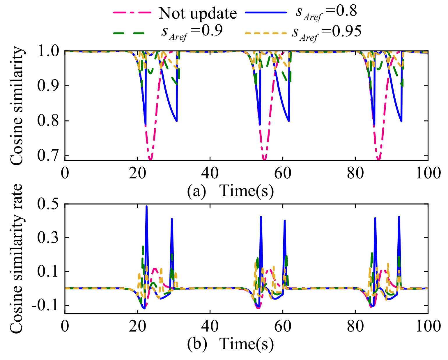
In order to better analyze the update frequency of the state matrix under different thresholds, we use the sine longitudinal velocity shown in Figure 19 as the speed input. The update threshold $s_{Aref}$ of cosine similarity is set as 0.8, 0.9, 0.95 and the non-updated state matrix.

As depicted in Figure 20, when the state matrix is not updated, the value of cosine similarity is small, while the rate of change of cosine similarity is large. From this perspective, the slight cosine similarity between the real-time longitudinal speed and the controller default state matrix causes the vehicle driving instability. When we set the threshold to 0.8, the overall cosine similarity decreases, and the number of updates is 6, but the rate of change becomes more extensive, to the detriment of the system input. When the update threshold is increased to 0.9, the rate of change of cosine similarity and the cosine similarity decrease, and the number of updates does not increase, remaining at 6. Continuing to increase to 0.95, the number of updates increases to 12, but the change rate of cosine similarity and the cosine similarity are further reduced. If continuing to increase the update threshold, the calculation load will further increase. After careful consideration, we set the update threshold of the state matrix as 0.9, which improves the real-time performance of the LQR controller without increasing the computation too much.

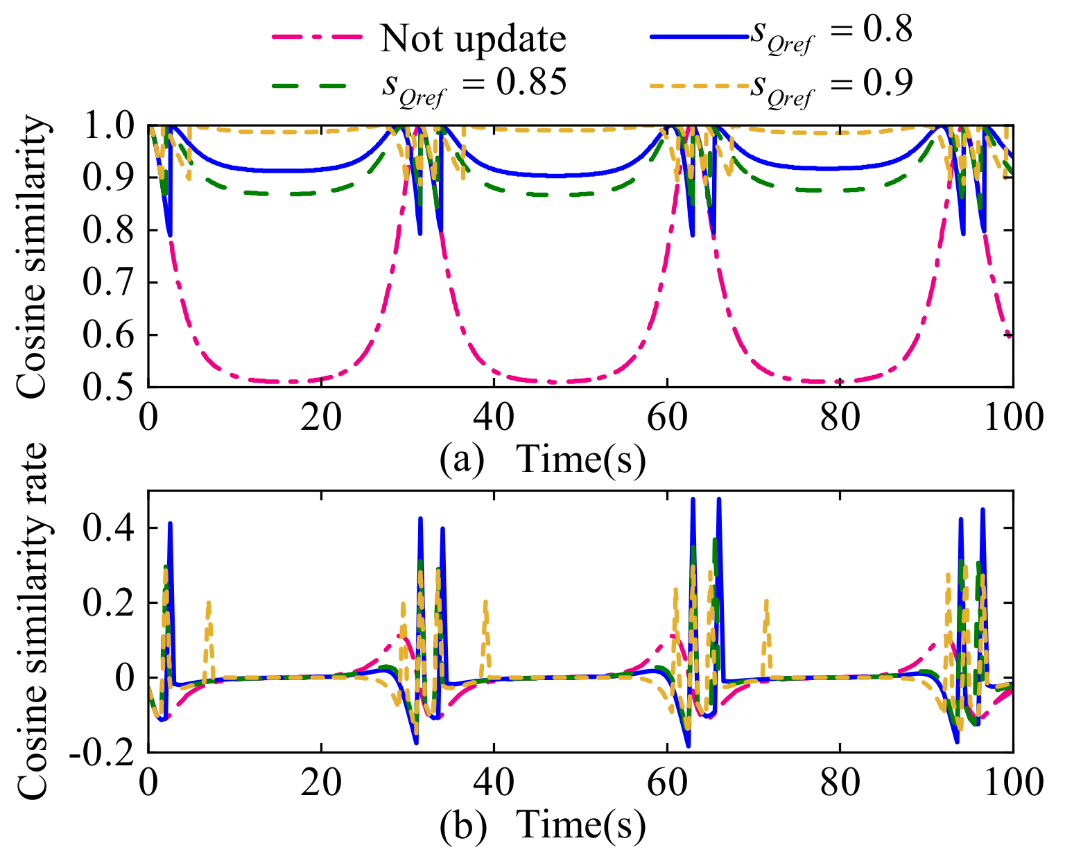
Through the same method used to analyze the selection of the update threshold of the weight coefficient matrix, we use the input shown in Figure 21 as the value for $\tau$ and $\sigma$. The update threshold $s_{Qref}$ of cosine similarity is set as 0.8, 0.85, 0.9 and the non-updated weight coefficient matrix.

As shown in Figure 22, when the weight coefficient matrix of the system is not updated, the cosine similarity is tiny, which cannot fulfill the vehicle’s adaptability to various situations. When we set the update threshold to 0.8, the overall cosine similarity decreases, and the number of updates is 7, but the rate of change becomes larger, which is not conducive to the system’s stability. When the update threshold is increased to 0.85, the rate of change of the cosine similarity and the cosine similarity decrease, which are in an appropriate range, and the number of updates is kept at 7. If continuing to increase to 0.9, the rate of change of cosine similarity and the cosine similarity are further reduced, but the number of updates increases by 14 times. If we continue to increase the update threshold, the calculation load will further increase. After comprehensive consideration, we set the update threshold of the state matrix as 0.85.

5. Simulation Results and Discussion

In order to verify the tracking performance of the improved LQR controller, we use the Simulink–Carsim platform for simulation verification. In the model shown in Figure 23, the Simulink software is applied to build the architecture of the lateral path tracking controller, and the Carsim software is used to build the vehicle model. We use the double lane change path as the desired path to test the tracking performance of the controller.

Table 3. Parameters for simulations.

Definition	Symbol	Value (Unit)
Vehicle mass	$m$	1412 (kg)
Moment of inertia about the Z-axis	$I_z$	1536.7 ($\mathrm{kg}\cdot {\mathrm{m}}^2$)
Distance from the centroid to the front axle	$l_f$	1.015 (m)
Distance from the centroid to the rear axle	$l_r$	1.895 (m)
Front-wheel turning stiffness	$C_{\alpha f}$	−148,970 ($\mathrm{N}\cdot {\mathrm{rad}}^{-1}$)
Rear-wheel turning stiffness	$C_{\alpha r}$	−82,204 ($\mathrm{N}\cdot {\mathrm{rad}}^{-1}$)
Input weight coefficient	$r$	20 (-)

lists the main parameters of the vehicle and controller.

We compare the improved LQR controller with the real-time updated LQR controller and test it in the case of speeds of 15 m/s and 25 m/s, respectively. In Figure 24, when the velocity is 15 m/s, the improved LQR controller’s tracking performance is as good as that of the real-time updated LQR controller. At low speeds, the maximum lateral error is about 0.2 m, which is a small and acceptable result. Although the improved LQR controller does not calculate and solve in real time, its tracking performance is ideal, with little deviation compared to the real-time updated LQR controller.

Figure 25 depicts the tracking performance of the improved LQR controller and the real-time updated LQR controller at the velocity of 25 m/s. When the vehicle is driving at high speeds, it is a challenge for the vehicle to drive perfectly on the double-lane change lane. At the turn with the immense curvature, the two control algorithms both have enormous errors. However, the lateral error of the improved LQR controller is smaller, and the vehicle can quickly correct the current state when the error is larger. Compared with the real-time updated LQR controller, the maximum lateral error of the improved LQR controller is reduced by about 28%. This shows that the improved LQR controller can reduce the error more effectively and make the vehicle drive in a safe condition when the tracking error of the vehicle is large. The main reason is that when the lateral error is large, the fuzzy controller adjusts the priority of the lateral error by adjusting the weight coefficient so that the LQR controller can eliminate the lateral error faster.

To evaluate the burden of the improved LQR controller on the computer, the computing time of the improved LQR controller is compared with that of the real-time updated LQR controller. The tic and toc functions in Matlab were used to record the computing time of different controllers at the velocity of 25 m/s, and the result is shown in Figure 26. The computing time of the improved LQR controller is reduced, which is 92% less than that of the real-time updated LQR controller. Meanwhile, the computing time has suddenly been increased at some time. The reason for this is that the cosine similarity is lower than the update threshold at these moments, leading to the controller’s recalculation. We can conclude that, due to the introduction of the calculation of the cosine similarity, the computing time of the improved LQR controller is significantly diminished most times, and the desired goal is achieved.

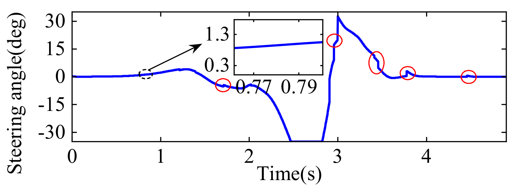
Figure 27 contains the steering angle information of the vehicle obtained by the improved LQR controller at a speed of 25 m/s. Compared with the steering angle in Figure 9, the steering angle here becomes smoother. We have revised the calculation method of the projection point to make the calculation of the projection point more accurate. However, there are still some sudden changes in the steering angle at the circles in Figure 27. The reason for this phenomenon is that the feedback coefficients obtained from the LQR scheme change abruptly after the fuzzy control updates the weighting coefficients.

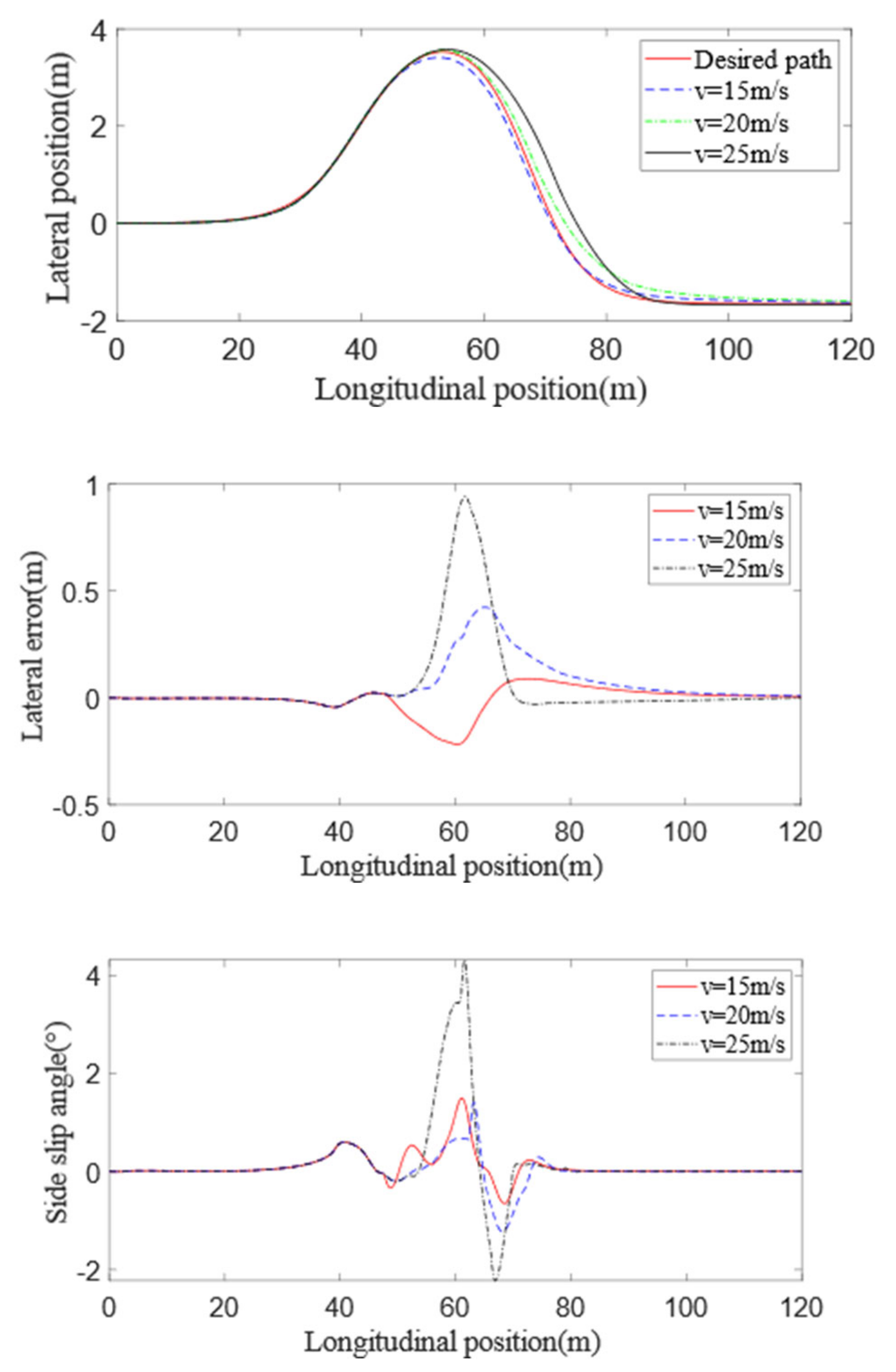
To study the accuracy of the improved LQR controller and its robustness with respect to speed, our comparison of simulation conditions at different vehicle speeds is shown in Figure 28. From the figure, we can see that when the vehicle’s velocity reaches 15 m/s and 20 m/s, it can follow the predetermined path better, which shows that the robustness of the controller is better. However, when the vehicle travels to a distance of 60 to 80 m, under the condition of 20 m/s, the lateral error of the vehicle increases to about 0.5 m, but the change in the side slip angle is not large, and the maximum is only about 1.5°. The vehicle runs smoothly. This indicates that the accuracy of the controller is greatly affected by the speed, but the stability is good. In general, the robustness, accuracy and stability of this improved LQR controller are acceptable under the condition that the vehicle speed is not too fast.

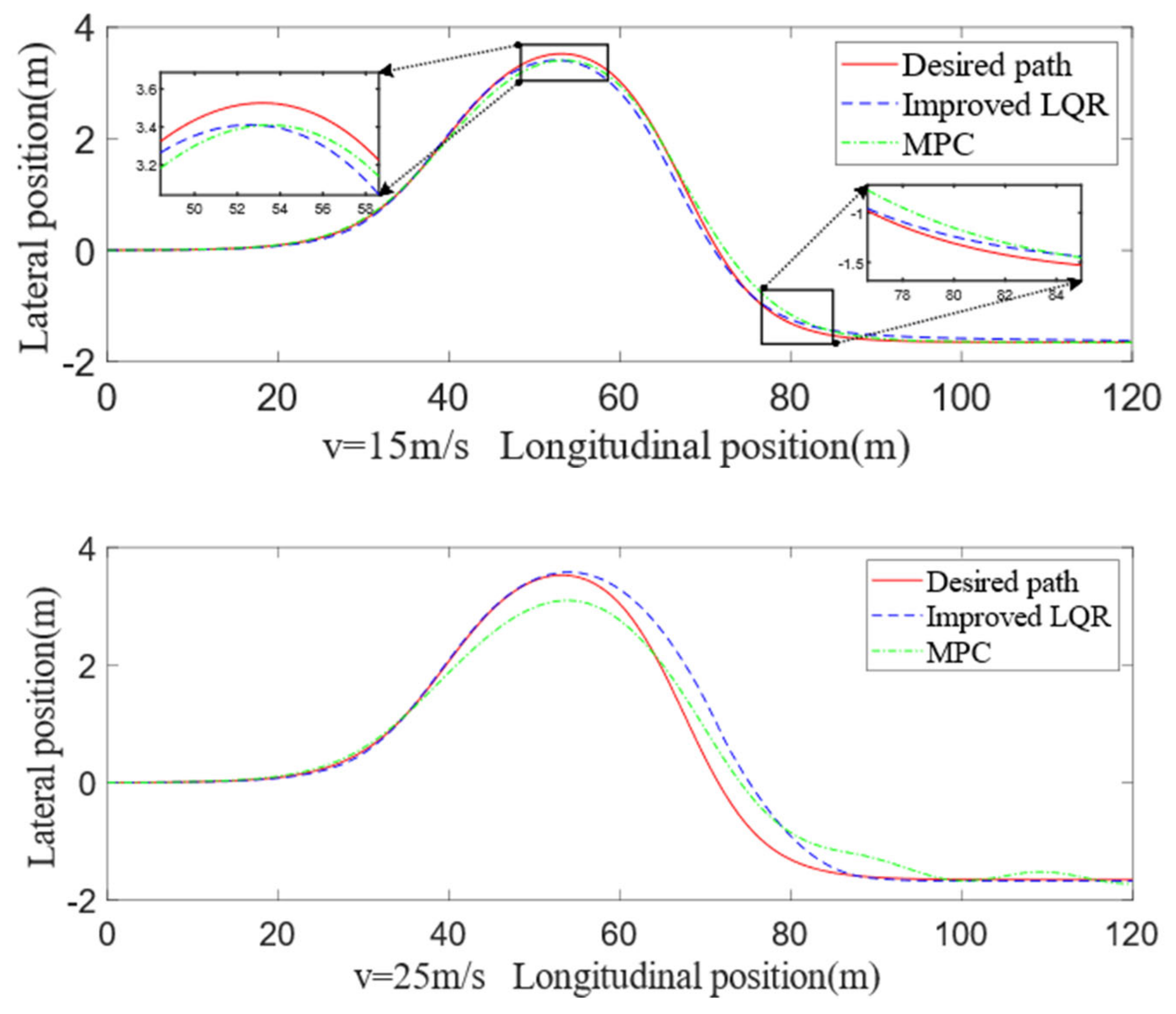
In order to study the performance of the designed controller, we compared the tracking effect with the model predictive (MPC) controller. The main parameters of the MPC controller are as follows: simulation step size $T_s=0.02 \mathrm{s}$, prediction step size $N_p=25$, control step size $N_c=10$, relaxation factor $\rho =100$, weight matrix $R=5\times {10}^5$.

The comparison results of two different controllers are shown in Figure 29. From Figure 29, we can see that the tracking performance of our designed LQR controller is better than that of the MPC controller when the vehicle speed is 15 m/s. Under the condition of the vehicle speed being 25 m/s, both controllers deviate from the planned path. At the same time, the vehicle under the control of the MPC controller exhibits oscillating motion. Therefore, the improved LQR controller we designed is better than the general MPC controller.

With the above test results and data, the path tracking effect of the improved LQR controller is verified to achieve the original design purpose. Compared with the real-time updated LQR controller, it can improve the adaptability of the vehicle, reduce the vehicle tracking error and decrease the computational load of the controller. Meanwhile, the vehicle path tracking accuracy can be improved compared with the fixed non-updating LQR controller. In addition, its performance effect is superior than that of the MPC controller. On the other hand, the adjustment of the weight coefficient can cause the steering angle to change drastically sometimes. When the tracking error deviation is huge, the steering angle needs to be adjusted to quickly reduce the tracking error, so the steering angle suddenly changes dramatically. Nevertheless, in most driving environments, the steering angle fluctuation will be minimal. However, the improved LQR controller proposed in this paper is based on two theories: fuzzy control theory and cosine similarity theory. There are two main limitations of this controller: (1) The choice of fuzzy control rules and membership functions is largely dependent on the experience and the lack of a corresponding theoretical basis. The fuzzy subset we chose is {NB, NS, ZO, PS, PB}, but other fuzzy subsets such as {NB, NM, NS, ZO, PS, PM, PB} are also available. The choice of different fuzzy subsets also produces different effects, so this is one of the disadvantages of the controller we designed. (2) The setting of the update threshold in the real-time update strategy based on cosine similarity is also selected by us through experiments and comprehensive consideration. This method is affected by human factors, which will affect the tracking accuracy.

6. Conclusions

In this paper, we propose an improved LQR-based lateral path tracking controller. First, the vehicle dynamics error model is established based on the Frenet coordinate system and the dynamics model. Then, we design the discrete LQR controller using the LaGrange multiplier method. At the same time, we analyzed and discussed the effect of each weight coefficient in the LQR controller on the tracking accuracy and steering angle. Therefore, we adopted a new method to calculate the coordinate information of the actual projection points to improve the steering stability. Fuzzy control is used to adjust the weight coefficients of the LQR controller to improve the tracking accuracy and adaptiveness of the vehicle under high-speed conditions. Simultaneously, the update rule of cosine similarity is proposed to improve the computational efficiency. Lastly, the improved LQR controller is compared and validated by using a real-time updated LQR controller. The results show that the improved LQR controller can reduce the tracking error more significantly in the case of large tracking errors.

This study decreases the computational load of the LQR controller while maintaining the tracking accuracy and stability, demonstrating the potential of the proposed strategy. Yet, some related issues still need further discussion and solutions: (1) The adjustment of the membership function and weight coefficients of the fuzzy controller is set by human experience, and its mathematical theory needs further research and proof. (2) Although the simulation experiments prove the reliability of the results, they still need to be tested in realistic scenarios. With the continuous progress of intelligent algorithms, advanced machine learning and intelligent optimization algorithms will be further integrated into future path tracking control research to design more accurate and efficient path tracking controllers.