Abstract
Parkinson’s disease (PD) is a neurodegenerative condition that affects the correct functioning of the motor system in the human body. Patients exhibit a reduced capability to produce facial expressions (FEs) among different symptoms, namely hypomimia. Being a disease so hard to be detected in its early stages, automatic systems can be created to help physicians in assessing and screening patients using basic bio-markers. In this paper, we present several experiments where features are extracted from images of FEs produced by PD patients and healthy controls. Classical machine learning methods such as local binary patterns and histograms of oriented gradients are used to model the images. Similarly, a well-known classification method, namely support vector machine is used for the discrimination between PD patients and healthy subjects. The most informative regions of the faces are found with a principal component analysis algorithm. Three different FEs were modeled: angry, happy, and surprise. Good results were obtained in most of the cases; however, happiness was the one that yielded better results, with accuracies of up to 80.4%. The methods used in this paper are classical and well-known by the research community; however, their main advantage is that they provide clear interpretability, which is valuable for many researchers and especially for clinicians. This work can be considered as a good baseline such that motivates other researchers to propose new methodologies that yield better results while keep the characteristic of providing interpretability.
Keywords:
Parkinson’s Disease; image processing; hypomimia; FE; classic techniques; machine learning 1. Introduction
Parkinson’s disease (PD) is a neurodegenerative condition that affects the basal ganglia, and it is responsible for the correct functioning of the cortical and sub-cortical motor systems. PD patients often exhibit reduced facial expressivity and develop difficulties producing facial expressions (FEs). The cortical motor system modulates expressions that are executed with consciousness, while the sub-cortical one is related to genuine expressional expressions which cannot be consciously moderated [1]. Studies suggest that PD patients show significantly less overall facial movement than healthy controls (HC) [2]. Reduced facial activity derives from impaired production of smiles and other expressions due to partial or permanent disabilities to move certain muscle groups, i.e., bradykinesia [3].
In the last decade, technological innovations have motivated the inclusion of machine learning (ML) techniques in different fields, including a diverse spectrum of topics within medicine [4,5,6]. ML contributes to this field by helping in medical assessments with predictive models that have been demonstrated to be accurate and reliable in a wide variety of applications [7,8]. Similarly, with the growth of ML methods, deep learning (DL) algorithms have been widely used thanks to the possibility to automatically extract features from raw data, perform the prepossessing and give a decision based on the data [9].
In [10], the authors showed that classical methods typically used to extract information and/or classify subjects, have been less used over years, while neural networks (NN) structures have increased their popularity. Although this is a global trend in many research areas, classical approaches can still yield good results. Classical models have a good performance with fewer computational requirements and offer the possibility to interpret the result, which is not possible in most of the cases where DL is used.
This paper intends to set a baseline for the automatic classification of PD patients and HC subjects. To this end, different FEs produced by the participants are modeled with classical and well-known feature extraction techniques including local binary patterns (LBP) and histograms of oriented gradients (HOG). Different expressions were studied including anger, happiness, and surprise. A support vector machine (SVM) was used as a classifier because it has been extensively used in other studies where FEs are modeled. Finally, an analysis of the regions that provide the most discriminant information was also performed.
2. Related Work
The interest in analyzing FEs in PD is growing in the ML community. One of the main challenges is to automatically detect the expression, which has been a hot topic in the past decade and multiple contributions have been done recently. For instance, In [11] proposed a method called Discriminative Kernel Facial Emotion Recognition (DKFER) which focuses on the integration of information from static facial features and motion-dependent features, the first set of features is extracted from a single image, the authors extracted landmarks of the faces of the Japanese Female FE (JAFFE) database [12] to obtain geometrical information; meanwhile, the motion dependent features are based on the Euclidean distance of the landmarks between the static state and the peak of the emotion, the result of this work was the definition of a new technique to merge both static and dynamic information.
One year later in [13], the authors extracted features using LBP from near-infrared (NIR) video sequences to classify different FEs, the authors used SVM and sparse representation classifier (SRC) and found that NIR videos help to reduce indoor light that changes depending on multiple factors and can affect the quality of the classification but has a drawback, which is that the working distance of NIR is limited. Later, the authors in [14] validated that there are a few facial muscles that are essential to discriminate different FEs. This result was achieved by extracting features from the Cohn–Kanade Database (CK+) [15] using LBP, which previously showed to be a powerful descriptor in FEs recognition [16].
In 2014, refs. [17,18] worked in understanding the contribution of different facial muscles in the performance of a FEs, and how this can be used to obtain a better classification of the FEs. The authors in [17] use landmarks to detect the main parts of the face such as the eyes, eyebrows corners, nose, and lip corners. The face is detected and later extracted using the Viola–Jones technique of Haar-like features [19]. The experiments were performed in both JAFFE and CK+ databases. The authors used an SVM as the classifier due to its simplicity and success in related works. On the other hand, the authors in [18] used only the CK+ database and proposed a new set of features called Muscle force-based features, which uses prior knowledge of facial anatomy to estimate the different activation levels of the muscles depending on the FEs. A wireframe model of the face, called HIgh polygon GEneric face Model (HI-GEM), originally introduced in [20] is used by the authors to extract information on key points of the face. Information on the involved muscles, forces, and direction are also extracted. Three classifiers are evaluated in [18], a Naive Bayes, an SVM, and a k-Nearest Neighbors (kNN). Better results were obtained with the SVM and KNN classification methods. Later, in [21] the authors extracted LBP and HOG features from both CK+ and JAFFE databases and found that different subjects have different ways to produce FEs, and such differences can be observed in LBP features, which makes this method a good feature extractor to model FEs. Other works such as [22,23,24,25,26,27,28] have used combinations of features, classifiers, and techniques to detect FEs; however, few works have addressed the problem of modeling FEs in PD patients. For instance, Bandini et al. [29] classified 17 PD patients and 17 HC subjects using landmarks extracted using information from the Microsoft Kinect Sensor. A Multi-Class SVM with a Gaussian kernel was trained for each expression: neutral, happiness, anger, disgust, and sadness. The classifiers were trained with the CK+ database and the Radboud Faces Database (RaFD) [30]. A 10-Fold Cross-Validation (CV) strategy was performed to optimize the meta-parameters of the classifiers, and the authors reported an average accuracy (ACC) of 88%. Specific results per expression indicate accuracies in test of 98% for happiness, 90% for disgust, 88% for anger, 84% for neutral, and 74% for sadness. In 2018 Rajnoha et al. [31] considered 50 PD patients and 50 HC subjects to automatically identify hypomimia through conventional classifiers such as random forest, XGBoost, and decision trees. The authors reported an average ACC of 67.33% in the classification between PD and HC subjects. One year later, Grammatikopoulou et al. [32] used similar features as the ones used by Bandini et al. to model FEs produced by 23 PD patients and 11 HC. The authors tried to classify three groups of subjects according to the FEs score in the MDS-UPDRS-III scale [33]. The Google Face API and Microsoft Face API were used to extract 8 facial landmarks and 27 facial landmarks, respectively. Two individual models were trained to estimate two Hypomimima Severity indexes (HSi1 for Google and HSi2 for Microsoft features). The authors reported a sensitivity of 0.79 and a specificity of 0.82 for the HSi1, while for HSi2 the results were 0.89 and 0.73, respectively. More recently, Jin et al. [34] used Face++ to automatically locate facial landmarks from an image, providing 106 landmark points. The work focused on the analysis of the tremor caused by movement disorders, which makes the key points tremble while trying to maintain the expression. The classification was performed with a long short-term memory (LSTM) and the authors reported accuracies of 86.76%.
Another recent contribution includes the one made by Gomez et al. [35]. In that work, the authors used the FacePark-GITA database, which includes a total of 54 participants (30 PD patients and 24 HC subjects). The authors implemented a multimodal study based on static and dynamic features. A set with 17 dynamic features was combined with 2048 static ones. They reported accuracies of 77.36% for static features and 71.15% for the dynamic ones. When the combination was considered the ACC improved to 88.76%. More recently, in 2021 the authors in [36] analyzed action units activation variance from Open-Face predictions. The three most relevant action units per expression were used to discriminate between PD patients and HC subjects by using an SVM classifier. The analysis was performed on 61 PD patients and 534 HC subjects of the PARK dataset [37]. The reported precision and recall were 95.8%, and 94.3%, respectively.
From the studies mentioned above, we observed that the use of landmarks and geometric features as well as classical classifiers are the most popular approaches and provide interpretable results. For this reason, in this paper we proposed to use LBP and HOG features to model FE produced by PD patients and HC subjects. Both methods are based on transformations over the images and return feature vectors widely used in FE recognition. Further analysis in classification stages can indicate which regions of the images may have influenced the decisions made. We are aware that there exist more sophisticated methods to perform FE analysis; however, we want to present this work as a rationale baseline for future studies. We expect other researchers to motivate to evaluate other methods, hopefully with better results but keeping a high level of interpretability, which is the strongest argument in favor of classical approaches.
3. Contributions of This Work
Two classical feature extraction techniques, LBP and HOG are used to extract features from video frames of PD patients and HC subjects who produced three different FEs, namely happiness, surprise, and angriness. An SVM classifier is considered to perform the classification between PD patients and HC subjects. The three FEs are modeled with the two feature extraction methods for comparison purposes. Furthermore, the information extracted from the features was analyzed to find those areas of the face that are more informative depending on the FEs and the feature extractor. This work can be considered as a baseline for the topic of considering FEs to discriminate between PD and HC subjects.
4. Methods
4.1. Methodology
Video recordings from both PD and HC groups will be separated into frames, from which only five frames will be used according to the findings reported in [35]. The sequence consisted of five images: Normal, Onset, Apex, Offset, and Normal, as shown in Figure 1.
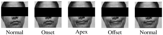
Figure 1.
Sequence of frames selected for each subject.
The face was extracted from each frame using the multi-task cascaded convolutional networks (MTCNN) algorithm, which removes the background noise to avoid unnecessary variability. The resulting image is resized to 80 × 80 pixels, gray-scaled, and normalized using facial landmarks as shown in Figure 2.
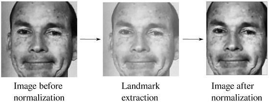
Figure 2.
Normalization process using Landmarks.
LBP and HOG features were extracted. For LBP, the image is transformed and divided into 20 × 20 sectors, for each sector the histogram is calculated and concatenated to form a 4096-dimensional feature vector (16 sectors × 256 values of the histograms). This process is illustrated in Figure 3.
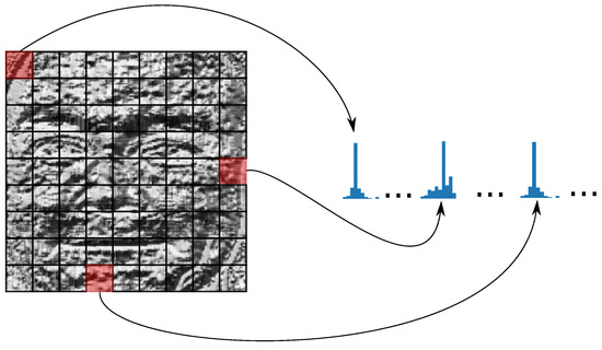
Figure 3.
LBP feature extraction.
In the case of HOG, the algorithm requires the number of pixels per cell in one of the parameters, which is set to 20 × 20 to use the same separation grid as the one used in LBP. For each block, eight orientations are extracted, then a principal component analysis (PCA) transformation with 95% of the variance is performed to select the most relevant features and to perform an analysis that allows the identification of areas in the face that are relevant for each expression. To achieve this, we check the coefficients found in the PCA transformation, the magnitudes of these coefficients give an idea of the relevance of each original feature in the new set of features.
The resulting features are then mapped back to the original image to identify the portion within the image from which it was extracted, a histogram with the contribution of each feature to the PCA transformation is created and reshaped to a 4 × 4 matrix, and later resized into an 80 × 80 image to show the areas of the faces that are selected the most.
4.2. Participants and Data Collection
The corpus considered for this work includes 31 PD patients and 23 HC subjects. All participants gave informed consent to participate in the study. Patients performed a variety of tasks including speech production, handwriting, gait, and the posed FEs exercises. Only the tasks about producing FEs are considered in this work. After completing those tasks, each patient visited the neurologist, who administered the MDS-UPDRS-III scale and provided the resulting scores. In the FEs tasks, patients were asked to imitate a specific expression presented by an avatar on a screen. For this study videos of angriness, surprise and happiness were considered. Figure 4 and Figure 5 show the distribution of demographic and clinical information of the participants, more detailed information can be found in Table 1. Possible biases due to age and gender were discarded according to a Welch’s t-test (p = 0.16) and a chi-square test (p = 0.57), respectively. All patients were recorded in ON-state, i.e., no more than 3 h after the medication intake.
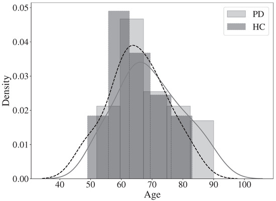
Figure 4.
Age distribution for both HC and PD.
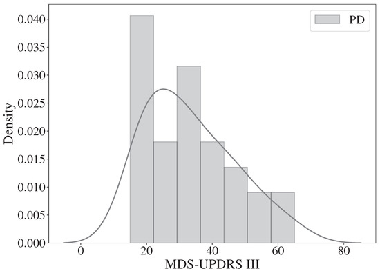
Figure 5.
Label count for the MDS-UPDRS-III scale.

Table 1.
Demographic information of the patients and healthy controls considered in this study.
4.3. Multi-Task Cascaded Convolutional Networks
Face detection is the first step before removing environmental noise, allowing the system to focus on the subjects’ faces. Cascade classifiers are commonly used for this aim. These methods consider features based on pixel intensities on images. For example, weighted classifiers detect contrasting face parts, such as the nose bridge and eyes. The algorithms work through small classifiers that ensemble a more robust one by detecting a face multiple times using different filters; the lower the complexity of the aforementioned small classifiers the more efficient the resulting system.
Multi-Task convolutional networks implement a novel and efficient approach to detect faces in images. The image is first resized multiple times in what is called an image pyramid, these resized images are then passed through a three-stage cascade network P-Net, R-Net, and O-Net [38]. P-Net is used to localize possible windows where a face can be found, the other two networks focus on the refinement and final decision of the window and its bounding boxes, as shown in Figure 6.
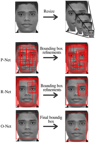
Figure 6.
MTCNN sequence to find a face in an image.
4.4. Local Binary Patterns
LBP is a visual descriptor-based method that considers differences between pixel neighborhoods to recognize features in images. The workflow of this method is as follows:
- The image color space is set to gray-scale.
- A radius hyper-parameter is chosen and the image is divided into cells.
- The central pixel of each cell is compared against its N neighbors. If the intensity of the center pixel is greater than or equal then a value of 1 is set in the neighbors’ position, otherwise, the value is set to 0.
- Starting clockwise from the top-right (Figure 7) a binary number is formed with the 1 s and 0 s from the previous step, this binary representation is then converted into decimal and stored in the central pixel position.
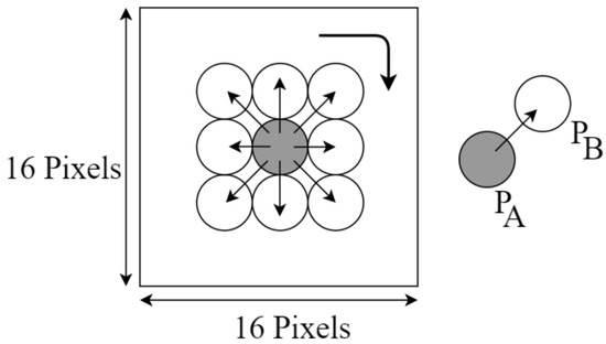 Figure 7. Neighbors operation in LBP.
 - With this new representation a feature histogram is formed.
- The process is repeated for each region and the histograms are concatenated forming the feature vector.
4.5. Histogram of Oriented Gradients
HOG considers shapes, objects, and textures by computing the intensity and direction of gradients [39]. The flow of this algorithm is as follows:
- The image color space is set to gray-scale.
- For each pixel in the image, the gradient is calculated in the x and y axes, generating and
- The magnitude and angle are calculated as shown in Equation (1):
- The gradient matrix is divided into cells where the histogram is calculated.
- Each histogram is normalized across local groups of cells using the normalization. This step is necessary to compensate for different changes in illumination and contrast between neighboring cells.
- An x-dimensional feature vector is computed across the resulting histograms.
The resulting vector is the one that will be used as a feature vector for the classification process, but we can also see how the magnitudes and angles change depending on the parameters, Figure 8 shows an example of an image where HOG was applied.
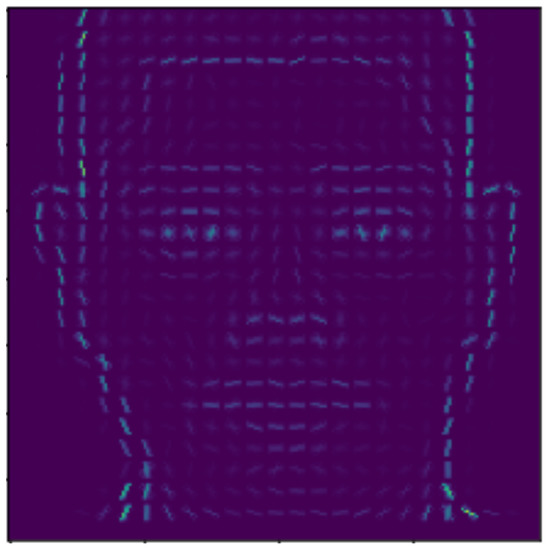
Figure 8.
Gradients obtained by the HOG algorithm.
4.6. Landmarks
A landmark is a point of correspondence that “matches between and within populations” [40]. This set of points raised the interest of researchers due to its successful use in face and FEs recognition [41]. The commonly used landmarks are focused in areas around the eyes, nose tip, nostrils, mouth, ears, and chin. A total of 68 landmarks are typically used to improve the representation of the face. External landmarks are also used to normalize the image. In this work, the pre-trained facial landmark detector introduced in [42] is used to estimate the 68 landmarks.
4.7. Principal Component Analysis (PCA)
PCA is a well-known transformation method commonly used to reduce the dimensionality of a large dataset. It can also be used to perform a feature selection that allows identifying which are the most relevant features in a given problem. PCA intends to capture the data with the most variance [43], and components that give less information are removed. The data are transformed through a linear combination of the variables, as shown in Equation (2):
where the original set of features and is the new set of features created with the linearly combination between and the constant values , where and with p and d are the original dimensionality and the new dimensionality respectively. After the transformation, there will be a linear combination of the original feature set multiplied by a constant for each principal component. Such a constant value can be considered as the “weight” for each feature.
4.8. Support Vector Machine (SVM)
SVM is a supervised machine learning method that focuses on finding the best margin or hyperplane that separates the data into two classes as shown in Figure 9. To find the best margin, an optimization process is performed by looking at the largest distance between the hyperplane and the data [44].
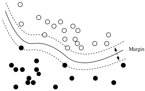
Figure 9.
Support vector machine.
The SVM intends to find the optimal hyperplane but the data are not always linearly separable. Therefore, kernels are implemented, and the main aim of a kernel is to transform the data into another space where the separability of the classes is linear. The kernel trick allows operating in the new space without mapping the data [45]. Some kernels are ( represents the feature matrix in all cases):
- Linear:
- Polynomial: , where d is the degree of the polynomial.
- Gaussian: , where is the kernel bandwidth.
- Sigmoid: , where r is a shifting parameter that controls the threshold of the mapping and is a scaling parameter for the input data [46].
SVM was selected as the classifier for this work given the fact that it has been extensively used in similar works where FEs are intended to be modeled. In fact, according to our literature revision, SVM is the classifier that most of the times yields better results. Another advantage of this classification method is its direct interpretability regarding the distance of the samples to the separating hyperplane.
5. Experiments and Results
5.1. Classification
The hyperparameters of the SVM are optimized following a subject-independent nested cross-validation strategy. This helps in reducing the bias when combining the hyper-parameter tuning and model selection. Given that each subject has five images for the outer loop of the nested cross-validation, stratified cross-validation is applied to split the dataset into train and test. These cross-validation method returns fold balanced in classes and with non-overlapping groups. Notice that in this case, the groups are each subject. A grid-search up to powers of ten where and is performed for the inner loop to obtain optimal parameters. shows the range of the hyper-parameter considered in the grid search. Optimal parameters used for the test are selected according to the mode along the training process. Notice that two different kernels are used, namely linear and Gaussian (also known as radial basis function—RBF).
5.2. Results
Table 2, Table 3 and Table 4 show both the parameters used in the classifier and the performance obtained, for the tree expressions the best feature extractor was LBP. The score distribution, as well as the ROC curve, are shown in Figure 10 and Figure 11.
Table 2.
PD classification results and optimal parameters analyzing angry expression.
Table 3.
PD classification results and optimal parameters in analyzing happiness expression.
Table 4.
PD classification results and optimal parameters analyzing surprise expression.
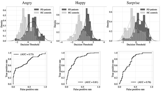
Figure 10.
Score distribution (Top) and ROC curve (Bottom).
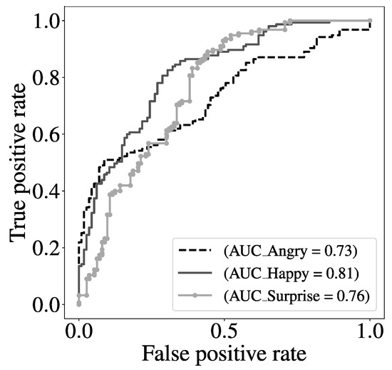
Figure 11.
ROC curve with the three expressions.
Apart from the classification experiments, statistical tests were performed to evaluate the distribution of the scores obtained with the classifier for each facial expression. First, a Shapiro–Wilk test was used to know whether the data follow a normal distribution. This test was performed for each class and facial expression, a total of six p-values were calculated (PD and HC in each emotion) and all of them were smaller than 0.05 which was the threshold to either reject or accept the null hypothesis. In this case, the test showed that none of the distributions are normal, so tests such as the t-test could not be applied. Nevertheless, another tests can be used e.g the Mann–Whitney U test. Table 5 shows the results of the Mann–Whitney U test and also whether the null hypothesis was rejected or not.
Table 5.
Mann–Whitney U tests to compare the scores obtained from the classifier per emotion.
After classifying the subjects, it is important to discuss what are the most relevant zones for both feature extractors in all expressions, this can be later compared with the classifier performance to understand which information is being considered by the classifiers to make the final decision. For both anger and surprise, we can notice that LBP shows more emphasis on the upper part of the face, while HOG focuses more on the eyes for both cases, as observed in Figure 12 and Figure 13. This behavior is somewhat expected because when the patient is performing the facial expression, these zones that change due to the facial expression are considered the zones with more variance and hence, the ones that stand out when the PCA algorithm is applied.
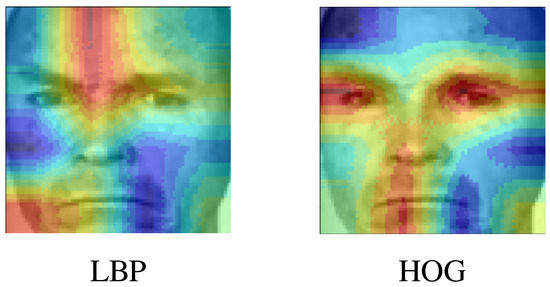
Figure 12.
Most important zones of the faces for angry.
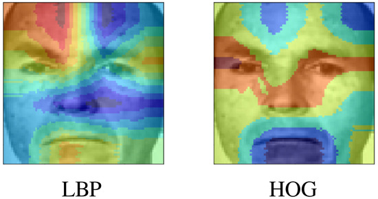
Figure 13.
Most important zones of the faces for surprise.
For the case of happiness, both feature extractors focus on the lower part of the face, LBP focuses more on the mouth region, while HOG focuses more on the cheek regions as seen in Figure 14. Both regions are the main regions involved in happiness expression. This show that both extractors when a PCA is applied can focus on different facial parts depending on the expression.
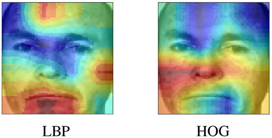
Figure 14.
Most important zones of the faces for happy.
6. Discusion
This study covers the analysis of FEs in PD using HOG and LBP features. The objective was to classify PD patients vs. HC subjects. 31 PD patients and 24 HC subjects were considered for the classification task. 55 videos were used for each expression. For each patient, five images are used, following the pattern: Normal, Onset, Apex, Offset, and Normal. A PCA reduction with a variance ratio of 95% is applied to remove redundant features and analyze these features to identify where the most important features are placed. Each feature set was considered separately for the classification tasks. An SVM classifier is considered. Nested cross-validation was used to optimize hyper-parameters and divide the dataset into train and test. The best result for anger has an ACC = 72.8%, for surprise, the classifier had an accuracy of 75.8%, and happiness an accuracy of 80.4%, making it the best facial expression for the classification of PD vs. HC.
The results in this work could relate to [29], a similar behavior was experimented with these expressions, although the validation scheme and features are different. This is an exploratory analysis of FEs in PD using classical approaches. The performance of the models proved to be adequate and robust to classify impaired expressions (i.e., models with ACC = 80.0%) despite the PDs with low UPDRS values.
The focus of this work is not only to be able to classify PD patients vs. HC subjects, but to perform a more detailed of the results and to understand what the classifier is seeking in order to separate the classes.
Further research is needed with more expressions to find out which is the most suitable for this task, as well as extracting features using deep learning architecture such as convolutional neural network (CNN), which has been widely used to automatically extract information from an image, this information can be compared with the hand-crafted features extracted in this work and also a combination of this features can be performed in order to improve the performance of the models. There is also a need for experiments related to clinical personnel to find which features are more suitable for clinical evaluations and find possible clinical interpretations of the results obtained with these models.
7. Limitations and Constraints
The main limitation of this work is the use of classical techniques both for feature extraction and for classification. We are aware that there exist more sophisticated methods in the literature such as those based on deep learning; however, we believe that classical methods have been overshadowed in the last few years, mostly because deep learning models require much less knowledge about the application (in the particular case of this paper, Parkinson’s disease and hypomimia), and achieve better results. The main point in favor of classical approaches is their interpretability (at the features and classification levels), which makes them more attractive for clinical applications in the real world. Another limitation of this study is the small size of the corpus. Although according to the literature revision the number of patients considered in this study is within the average, we are aware that more data would help in finding more conclusive results. Notice that this limitation also supports the fact of not using DL methods, because these approaches require much more data than the classical ones.
8. Conclusions
The production of FEs is a sensible bio-marker for the classification between PD patients and HC subjects. Given the fact that different muscles are activated depending on which FE to be produced, accurate and interpretable models able to extract information from different FEs are necessary. This work presents a study where classical yet interpretable techniques are used to create models that allow the automatic discrimination between PD patients and HC subjects. The classifier used in this study showed high sensitivity in most of the cases. However, the specificity decreased when the HOG features were considered. This is possibly due to similarities between the facial abilities of some HC subjects and PD patients who were in a low to intermediate state of the disease. The normalization performed with Landmarks reduced the variability of the background which helped in reducing errors when the models were focusing on the important zones. Regarding the different FEs produced by the patients, happiness has yielded the highest accuracy; however, the results obtained with the other two FEs suggest that the three of them can be used to perform the classification and obtain better results. LBP shows the best results for the three FEs, although the zones highlighted with HOG features are also interesting to look at. The main contribution of this work is to set a baseline with classical and interpretable methods such that motivate other researchers to study other approaches that likely yield also interpretable results with higher accuracies. Although the results in this work cannot be directly compared to those in the state-of-the-art because the datasets are different, we believe that in terms of classical approaches, the results presented here are competitive and result in a good baseline model. Future studies should focus on developing more sophisticated methodologies that provide better classification results while keeping a clear interpretability for clinicians, patients, and caregivers.
Author Contributions
Conceptualization, N.R.C.-A., L.F.G.-G. and J.R.O.-A.; methodology, N.R.C.-A. and L.F.G.-G.; validation, N.R.C.-A. and L.F.G.-G.; formal analysis, N.R.C.-A., L.F.G.-G. and J.R.O.-A.; investigation, L.F.G.-G.; resources, L.F.G.-G. and J.R.O.-A.; data curation, N.R.C.-A. and L.F.G.-G.; writing—original draft preparation, N.R.C.-A.; writing—review and editing, N.R.C.-A., L.F.G.-G. and J.R.O.-A.; visualization, N.R.C.-A.; supervision, L.F.G.-G. and J.R.O.-A.; project administration, J.R.O.-A.; funding acquisition, J.R.O.-A. All authors have read and agreed to the published version of the manuscript.
Funding
The study was partially funded by CODI at Universidad de Antioquia grant # PRG2017-15530 and by the planning direction and institutional development at Universidad de Antioquia, project # ES92210001.
Institutional Review Board Statement
This study was approved by the Ethical Research Committee of the University of Antioquia and according to the Helsinki declaration (1964) and its later amendments.
Informed Consent Statement
Written informed consent has been obtained from the patient(s) to publish this paper.
Data Availability Statement
Not applicable.
Acknowledgments
The authors would like to thank the patients of the Parkinson’s Foundation in Medellín, Colombia (Fundalianza https://www.fundalianzaparkinson.org/) for their cooperation during the development of this study. Without their contribution, it would have been impossible to address this work.
Conflicts of Interest
The authors declare no conflict of interest. The funders had no role in the design of the study; in the collection, analyses, or interpretation of data; in the writing of the manuscript; or in the decision to publish the results.
References
- Rinn, W. The neuropsychology of facial expression: A review of the neurological and psychological mechanisms for producing facial expressions. Psychol. Bull. 1984, 95, 52–77. [Google Scholar] [CrossRef] [PubMed]
- Smith, M.C.; Smith, M.K.; Ellgring, H. Spontaneous and posed facial expression in Parkinson’s Disease. J. Int. Neuropsychol. Soc. 1996, 2, 383–391. [Google Scholar] [CrossRef] [PubMed]
- Bologna, M.; Fabbrini, G.; Marsili, L.; Defazio, G.; Thompson, P.D.; Berardelli, A. Facial bradykinesia. J. Neurol. Neurosurg. Psychiatry 2013, 84, 681–685. [Google Scholar] [CrossRef] [PubMed]
- Dargan, S.; Kumar, M.; Ayyagari, M.R.; Kumar, G. A Survey of Deep Learning and Its Applications: A New Paradigm to Machine Learning. Arch. Comput. Methods Eng. 2020, 27, 1071–1092. [Google Scholar] [CrossRef]
- Prakash, A.J.; Ari, S. A system for automatic cardiac arrhythmia recognition using electrocardiogram signal. Bioelectron. Med. Devices 2019, 2019, 891–911. [Google Scholar]
- Safi, K.; Fouad Aly, W.H.; AlAkkoumi, M.; Kanj, H.; Ghedira, M.; Hutin, E. EMD-Based Method for Supervised Classification of Parkinson’s Disease Patients Using Balance Control Data. Bioengineering 2022, 9, 283. [Google Scholar] [CrossRef]
- Schwartz, W.; Patil, R.; Szolovits, P. Artificial intelligence in medicine. Where do we stand? N. Engl. J. Med. 1987, 316, 685–688. [Google Scholar] [CrossRef]
- Deo, R.C. Machine Learning in Medicine. Circulation 2015, 132, 1920–1930. [Google Scholar] [CrossRef]
- LeCun, Y.; Bengio, Y.; Hinton, G. Deep learning. Nature 2015, 521, 436–444. [Google Scholar] [CrossRef]
- Canal, F.Z.; Müller, T.R.; Matias, J.C.; Scotton, G.G.; de Sa Junior, A.R.; Pozzebon, E.; Sobieranski, A.C. A survey on facial emotion recognition techniques: A state-of-the-art literature review. Inf. Sci. 2022, 582, 593–617. [Google Scholar] [CrossRef]
- Wang, H.; Huang, H.; Hu, Y.; Anderson, M.; Rollins, P.; Makedon, F. Emotion detection via discriminative kernel method. In Proceedings of the 3rd International Conference On Pervasive Technologies Related To Assistive Environments, Samos, Greece, 23–25 June 2010; pp. 1–7. [Google Scholar]
- Lyons, M.; Akamatsu, S.; Kamachi, M.; Gyoba, J. Coding facial expressions with gabor wavelets. In Proceedings of the Third IEEE International Conference on Automatic Face And Gesture Recognition, Nara, Japan, 14–16 April 1998; pp. 200–205. [Google Scholar]
- Zhao, G.; Huang, X.; Taini, M.; Li, S.Z.; PietikäInen, M. Facial expression recognition from near-infrared videos. Image Vis. Comput. 2011, 29, 607–619. [Google Scholar] [CrossRef]
- Zhong, L.; Liu, Q.; Yang, P.; Liu, B.; Huang, J.; Metaxas, D.N. Learning active facial patches for expression analysis. In Proceedings of the 2012 IEEE Conference on Computer Vision and Pattern Recognition, Providence, RI, USA, 16–21 June 2012; pp. 2562–2569. [Google Scholar]
- Lucey, P.; Cohn, J.; Kanade, T.; Saragih, J.; Ambadar, Z.; Matthews, I. The Extended Cohn-Kanade Dataset (CK+): A complete dataset for action unit and emotion-specified expression. In Proceedings of the 2010 IEEE Computer Society Conference on Computer Vision and Pattern Recognition-Workshops, San Francisco, CA, USA, 13–18 June 2010; pp. 94–101. [Google Scholar] [CrossRef]
- Shan, C.; Gong, S.; McOwan, P.W. Facial expression recognition based on local binary patterns: A comprehensive study. Image Vis. Comput. 2009, 27, 803–816. [Google Scholar] [CrossRef]
- Happy, S.; Routray, A. Automatic facial expression recognition using features of salient facial patches. IEEE Trans. Affect. Comput. 2014, 6, 1–12. [Google Scholar] [CrossRef]
- Eskil, M.T.; Benli, K.S. Facial expression recognition based on anatomy. Comput. Vis. Image Underst. 2014, 119, 1–14. [Google Scholar] [CrossRef]
- Viola, P.; Jones, M. Rapid object detection using a boosted cascade of simple features. In Proceedings of the 2001 IEEE Computer Society Conference On Computer Vision And Pattern Recognition, CVPR 2001, Kauai, HI, USA, 8–14 December 2001; Volume 1, p. I. [Google Scholar]
- Abeysundera, H.P.; Benli, K.S.; Eskil, M.T. Nearest neighbor weighted average customization for modeling faces. Mach. Vis. Appl. 2013, 24, 1525–1537. [Google Scholar] [CrossRef]
- Liu, Y.; Li, Y.; Ma, X.; Song, R. Facial expression recognition with fusion features extracted from salient facial areas. Sensors 2017, 17, 712. [Google Scholar] [CrossRef]
- Varma, S.; Shinde, M.; Chavan, S.S. Analysis of PCA and LDA features for facial expression recognition using SVM and HMM classifiers. In Techno-Societal 2018; Springer: Berlin/Heidelberg, Germany, 2020; pp. 109–119. [Google Scholar]
- Reddy, C.V.R.; Reddy, U.S.; Kishore, K.V.K. Facial emotion recognition using NLPCA and SVM. Trait. Signal 2019, 36, 13–22. [Google Scholar] [CrossRef]
- Nazir, M.; Jan, Z.; Sajjad, M. Facial expression recognition using histogram of oriented gradients based transformed features. Clust. Comput. 2018, 21, 539–548. [Google Scholar] [CrossRef]
- Acevedo, D.; Negri, P.; Buemi, M.E.; Fernández, F.G.; Mejail, M. A simple geometric-based descriptor for facial expression recognition. In Proceedings of the 2017 12th IEEE International Conference on Automatic Face & Gesture Recognition (FG 2017), Washington, DC, USA, 30 May–3 June 2017; pp. 802–808. [Google Scholar]
- Chaabane, S.B.; Hijji, M.; Harrabi, R.; Seddik, H. Face recognition based on statistical features and SVM classifier. Multimed. Tools Appl. 2022, 81, 8767–8784. [Google Scholar] [CrossRef]
- Bhangale, K.B.; Jadhav, K.M.; Shirke, Y.R. Robust pose invariant face recognition using DCP and LBP. Int. J. Manag. Technol. Eng. 2018, 8, 1026–1034. [Google Scholar]
- Eng, S.; Ali, H.; Cheah, A.; Chong, Y. Facial expression recognition in JAFFE and KDEF Datasets using histogram of oriented gradients and support vector machine. In Proceedings of the IOP Conference Series: Materials Science And Engineering; IOP Publishing: Bristol, UK, 2019; Volume 705, p. 012031. [Google Scholar]
- Bandini, A.; Orlandi, S.; Escalante, H.J.; Giovannelli, F.; Cincotta, M.; Reyes-Garcia, C.A.; Vanni, P.; Zaccara, G.; Manfredi, C. Analysis of facial expressions in parkinson’s disease through video-based automatic methods. J. Neurosci. Methods 2017, 281, 7–20. [Google Scholar] [CrossRef] [PubMed]
- Langner, O.; Dotsch, R.; Bijlstra, G.; Wigboldus, D.H.J.; Hawk, S.T.; van Knippenberg, A. Presentation and validation of the Radboud Faces Database. Cogn. Emot. 2010, 24, 1377–1388. [Google Scholar] [CrossRef]
- Rajnoha, M.; Mekyska, J.; Burget, R.; Eliasova, I.; Kostalova, M.; Rektorova, I. Towards Identification of Hypomimia in Parkinson’s Disease Based on Face Recognition Methods. In Proceedings of the 2018 10th International Congress on Ultra Modern Telecommunications and Control Systems and Workshops (ICUMT), Moscow, Russia, 5–9 November 2018; pp. 1–4. [Google Scholar] [CrossRef]
- Grammatikopoulou, A.; Grammalidis, N.; Bostantjopoulou, S.; Katsarou, Z. Detecting hypomimia symptoms by selfie photo analysis: For early Parkinson disease detection. In Proceedings of the 12th ACM International Conference on PErvasive Technologies Related to Assistive Environments, Island of Rhodes, Greece, 5–7 June 2019; pp. 517–522. [Google Scholar]
- Goetz, C.G.; Tilley, B.C.; Shaftman, S.R.; Stebbins, G.T.; Fahn, S.; Martinez-Martin, P.; Poewe, W.; Sampaio, C.; Stern, M.B.; Dodel, R.; et al. Movement Disorder Society-sponsored revision of the Unified Parkinson’s Disease Rating Scale (MDS-UPDRS): Scale presentation and clinimetric testing results. Mov. Disord. Off. J. Mov. Disord. Soc. 2008, 23, 2129–2170. [Google Scholar] [CrossRef] [PubMed]
- Jin, B.; Qu, Y.; Zhang, L.; Gao, Z. Diagnosing Parkinson disease through facial expression recognition: Video analysis. J. Med. Internet Res. 2020, 22, e18697. [Google Scholar] [CrossRef] [PubMed]
- Gómez-Gómez, L.F.; Morales, A.; Fierrez, J.; Orozco-Arroyave, J.R. Exploring Facial Expressions and Action Unit Domains for Parkinson Detection. SSRN 2022. [Google Scholar] [CrossRef]
- Ali, M.R.; Myers, T.; Wagner, E.; Ratnu, H.; Dorsey, E.; Hoque, E. Facial expressions can detect Parkinson’s disease: Preliminary evidence from videos collected online. NPJ Digit. Med. 2021, 4, 1–4. [Google Scholar] [CrossRef]
- Langevin, R.; Ali, M.R.; Sen, T.; Snyder, C.; Myers, T.; Dorsey, E.R.; Hoque, M.E. The PARK framework for automated analysis of Parkinson’s disease characteristics. Proc. ACM Interact. Mob. Wearable Ubiquitous Technol. 2019, 3, 1–22. [Google Scholar] [CrossRef]
- Zhang, K.; Zhang, Z.; Li, Z.; Qiao, Y. Joint face detection and alignment using multitask cascaded convolutional networks. IEEE Signal Process. Lett. 2016, 23, 1499–1503. [Google Scholar] [CrossRef]
- Dalal, N.; Triggs, B. Histograms of oriented gradients for human detection. In Proceedings of the 2005 IEEE Computer Society Conference On Computer Vision And Pattern Recognition (CVPR’05), San Diego, VA, USA, 20–25 June 2005; Volume 1, pp. 886–893. [Google Scholar]
- Dryden, I.L.; Mardia, K.V. Statistical Shape Analysis: With Applications in R; John Wiley & Sons: Hoboken, NJ, USA, 2016; Volume 995. [Google Scholar]
- Shi, J.; Samal, A.; Marx, D. How effective are landmarks and their geometry for face recognition? Comput. Vis. Image Underst. 2006, 102, 117–133. [Google Scholar] [CrossRef]
- Kazemi, V.; Sullivan, J. One millisecond face alignment with an ensemble of regression trees. In Proceedings of the IEEE Conference On Computer Vision And Pattern Recognition, Washington, DC, USA, 23–28 June 2014; pp. 1867–1874. [Google Scholar]
- Xu, Y.; Zhang, D.; Yang, J.Y. A feature extraction method for use with bimodal biometrics. Pattern Recognit. 2010, 43, 1106–1115. [Google Scholar] [CrossRef]
- Schölkopf, B.; Smola, A.J.; Bach, F. Learning with Kernels: Support Vector Machines, Regularization, Optimization, And Beyond; MIT Press: Cambridge, MA, USA, 2002. [Google Scholar]
- Soentpiet, R. Advances in Kernel Methods: Support Vector Learning; MIT Press: Cambridge, MA, USA, 1999. [Google Scholar]
- Lin, H.T.; Lin, C.J. A study on sigmoid kernels for SVM and the training of non-PSD kernels by SMO-type methods. Neural Comput. 2003, 3, 16. [Google Scholar]


Publisher’s Note: MDPI stays neutral with regard to jurisdictional claims in published maps and institutional affiliations. |
© 2022 by the authors. Licensee MDPI, Basel, Switzerland. This article is an open access article distributed under the terms and conditions of the Creative Commons Attribution (CC BY) license (https://creativecommons.org/licenses/by/4.0/).