Abstract
Integrated Energy Systems (IES) are an important way to improve the efficiency of energy, promote closer connections between various energy systems, and reduce carbon emissions. The transformation between electricity, heating, and cooling loads into each other makes the dynamic characteristics of multiple loads more complex and brings challenges to the accurate forecasting of multi-energy loads. In order to further improve the accuracy of IES short-term load forecasting, we propose the Convolutional Neural Network, the Long Short-Term Memory Network, and Auto-Regression (CLSTM-AR) combined with the multi-dimensional feature fusion (MFFCLA). In detail, CLSTM can extract the coupling and periodic characteristics implied in IES load data from multiple time dimensions. AR takes load data as the input to extract features of sequential auto-correlation over adjacent time periods. Then, the diverse and effective features extracted by CLSTM, LSTM, and AR can be fused using the multi-dimensional feature fusion technique. Ultimately, the model achieves the accurate prediction of multiple loads. In conclusion, compared with other forecasting models, the case study results show that MFFCLA has higher forecasting precision compared with the comparable model in the short-term multi-energy load forecasting performance of electricity, heating, and cooling. The accuracy of MFFCLA can help to optimize and dispatch IES to make better use of renewable energy.
1. Introduction
Aiming at the defects of the traditional energy supply system, IES—as an important way to improve energy efficiency—promotes the connection of various energy systems more closely and effectively reduces carbon emission [1]. IES uses electricity as a primary carrier of energy supply, and the energy supply systems are coordinated and optimized with each other. This advantage of flexible switching also makes the dynamic characteristics of multi-energy loads further complex [2]. Furthermore, a strongly coupled multi-energy system may increase the risk of system cascading failures [3]. Therefore, it is necessary to accurately predict the multi-energy load of the IES, which is the key to ensure the efficient and stable operation of the power supply equipment.
Short-term load forecasting is divided into traditional methods and artificial intelligence methods. In the traditional methods, the regression analysis algorithm represented by Auto-Regression Integrated Moving Average model (ARIMA) [4] and the machine learning models represented by Support Vector Machine (SVM) [5,6], Random Forest [7,8], XGBoost [9], and Sparse Algorithm [10] are used. With the increasing complexity of energy systems and the diversification of the energy demand, it is difficult to obtain satisfactory prediction targets using the regression analysis method. Although machine-learning algorithms can solve the above problems, they need to construct the temporal characteristics of the data artificially.
With the rapid development of artificial intelligence algorithms, long short-term memory networks (LSTMs) have significant advantages in solving time-series problems and have been studied in the field of electricity load forecasting in recent years [11,12]. The authors in [13] used LSTM combined with the improved sparrow search algorithm to predict short-term load. The authors in [14] proposed a combined LSTM and a self-attention mechanism model with two-input group channels for forecasting the day-ahead residential load. The mentioned LSTM individual load forecasting model was trained using a pinball loss-guided optimization approach [15]. The above-mentioned papers all constructed prediction models for a single load, and although they had high prediction accuracy, the models did not consider the coupling information implied between multi-energy loads. Therefore, the above models are not suited to the multi-energy load forecasting problem of IES.
Considering the complex coupling relationships among multi-energy loads, such as electricity, heating, and gas in IES, a wavelet neural network optimized by improved particle swarm optimization and the chaos optimization algorithm (WNN-IPSO-COA) was introduced to the short-term load forecasting of IES is proposed in [16]. A Variational Mode Decomposition (VMD) method was used to decompose the original data and remove the noise, which is helpful for the accuracy of the LSTM short-term load forecasting as proposed in [17]. Furthermore, Zhang and Bai adopted a sequence-to-sequence network based on an encoder–decoder architecture to enhance the load-timing feature-mining capability [18].
All of the above protocols perform IES load predicting from the single-task perspective, which does not consider the Multi-Task Learning (MTL) scenario [19]. To forecast electricity, heating, and cooling loads simultaneously, Tan and others proposed an MTL evolved from a Least Square Support Vector Machine (LSSVM) [20]. A Deep Belief Network (DBN) is based on a restricted Boltzmann machine for data feature extraction, and these features are fed to the MTL for load forecasting [21]. Although most of the aforementioned multi-energy load-forecasting methods consider the complex dynamic characteristics among energy sources, they do not thoroughly explore the important data information in more dimensions.
Load forecasting is a time-series correlation problem, where the load changes of IES depend on the antecedent state, which means that load changes are highly auto-correlated in time [22]. Although LSTM and GRU have great advantages in time series prediction, they cannot capture the short-term interdependence when the time sequence is too long [23]. Therefore, it is necessary not only to learn the relation of coupling between different loads of different time dimensions but also to strengthen the change relation between loads at adjacent times.
We propose a CLSTM-AR multi-energy load-forecasting method based on multi-dimensional feature fusion. The method can effectively learn the coupling relationship among different loads and enhance the time-series relation of the load itself. Eventually, the proposed MFFCLA will be able to greatly improve the accuracy of multi-energy load forecasting.
Our contributions can be summarized as follows. An auto-regression algorithm is used to store ultra-short time series state features of multi-energy loads using an LSTM neural network and mining the characteristics of weather factors in IES.
By combining a Convolutional Neural Network (CNN) and LSTM neural network, the spatial and temporal features of multiple time dimensions are extracted. The multidimensional feature fusion technique is applied to fuse the effective features of multiple dimensions extracted above, allowing the advantages of each feature to be exploited. The results verify that the proposed model has higher prediction accuracy compared with the existing ARIMA, LSTM, and CLSTM forecasting models.
The remainder of the paper is structured as follows. Section 2 analyzes the time-series auto-correlation of each load of the IES and the spatial correlation between different data. Section 3 first describes the overall framework of the model. Secondly, we construct multidimensional input features based on the analysis results and introduce AR, CLSTM, and LSTM feature extraction methods as well as multidimensional feature fusion techniques. Section 4 shows the experimental results of the algorithm and a comparison with other short-term load prediction models. Our conclusions are discussion in Section 5.
2. Characteristic Analysis of Integrated Energy SystemsIES
Integrated energy systems is a complex energy system integrated with energy production, supply, and consumption, which can coordinate and optimize different energy sources in the process of energy system planning, construction, and operation. The system operation brings a large amount of measurement information, and analysis of the system measurement data will produce general knowledge of the whole system and provide help in the construction of prediction models. For the spatial-temporal correlation information implied in the data, the auto-correlation coefficients function is used to analyze the temporal auto-correlation of the load data, and the spatial coupling characteristics between the data are analyzed using the Person correlation coefficient method.
The integrated energy system spatial and time-series characterization data consists of load data and weather data. Load data was obtained from the National Renewable Energy Laboratory website [24]. Weather data was obtained from the weather website of the region where the IES system is located [25]. The actual data are shown in Figure 1 (the weekday types are not listed separately because the values are only 0 and 1).
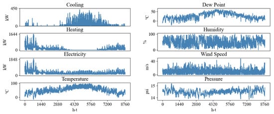
Figure 1.
IES year-round actual data.
In Figure 2, the blue area is the confidence range for the auto-correlation coefficient with a 90% confidence interval. Scatters then indicate that the delay time is 1 h with different delay times. Analysis of the auto-correlation coefficients within the first 4 h shows that the electricity, heating, and cooling loads are positively correlated and outside the confidence interval. The electricity and heating loads auto-correlation coefficients are negatively correlated outside the confidence interval at a lag of 8–16 h; the cooling loads are negatively correlated outside the confidence interval at a lag of 9–14 h.
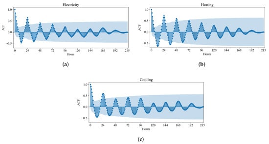
Figure 2.
The loads temporal auto-correlation. (a) The electricity load temporal auto-correlation. (b) The heating load temporal auto-correlation. (c) The cooling load temporal auto-correlation.
At 22–26 h, the auto-correlation coefficients of the electricity, heating, and cold loads are again outside the confidence interval and are positively correlated, while the coefficient values reach a peak in the direction of positive correlation at every 24 h interval. At the 168th hour, the electricity and cooling loads are more variable than in the first two cycles. After the 168th hour, the loads show less correlation than within a week. It can be seen that the load itself has continuous strong auto-correlation in the first 4 h, and the load data has both daily and weekly characteristics.
In the IES system, there is a mutual transformation and complementary characteristic between the individual energies, and this unclear coupling relationship affects the accurate accuracy of the power system to an extent. The correlation between the factors is analyzed by the Person correlation coefficient method, and the analysis results are plotted by heat map as shown in Figure 3.
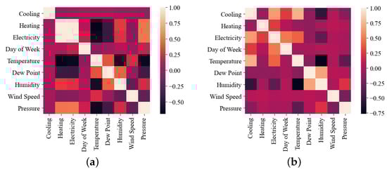
Figure 3.
Characteristics correlation analysis heat map. (a) The heating season, which is from January to May and from October to December. (b) The non-heating season, which is from June to September.
In Figure 3, the legend represents the correlation degree between attributes, and the coefficients take values in the range of [−1, 1]. When the coefficient is 0, it means that the two attributes are not correlated at all; when the coefficient is positive, it means that the attributes are positively correlated with each other; and when the coefficient is negative, they are negatively correlated. In Figure 3a, the coefficient of the electricity load and cooling load is 0.0236; the coefficient of the electricity load and heating load is 0.9828; and the coefficient of the heating load and cooling load is −0.0005.
In Figure 3b, the coefficient of the electricity load and cooling load is 0.6486; the coefficient of the electricity load and heating load is 0.2645; and the coefficient of the heating load and cooling load is −0.0441. Clearly, the electricity load has an extremely high correlation with the heat load during the heating season and the electricity load with the cold load during the non-heating season, which is related to the use of thermo-electrical device and heat-pump equipment in the building. Furthermore, temperature has a high correlation with the cooling and heating loads. The workday type is more closely related to the electricity load.
3. Proposed Model
There are coupling relationships between multiple energy systems in IES, and CNN has the ability to handle this spatially interactive information, while single-load prediction is a typical time-series problem, LSTM is able to consider the temporal periodicity of loads. On this basis, CNN and LSTM are connected in order to further improve the ability of the model for spatial-temporal feature mining of multi-energy load. Based on the results of auto-correlation analysis of the load data mentioned above, the time-varying of loads relies on the ultra-short-term priors state change, and the AR algorithm is used to store the load’s prior state. Considering the influence of weather factors on the energy consumption load, a LSTM is used to study the weather influence characteristics.
Figure 4 shows the overall framework. Data input module: the original time series data are constructed from multiple dimensions. Data feature extraction module: the data features are extracted from multiple perspectives by AR, CLSTM, and LSTM according to the characteristics of the input data. Multi-dimensional feature fusion prediction module: the extracted multi-dimensional abstract features are fused using Concatenate and Add layers, and finally load prediction is realized by fully connected layers.
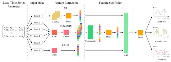
Figure 4.
Multi-energy load-forecasting model framework.
Model input and output settings, AR, CLSTM, and LSTM feature-extraction models and feature fusion are described in detail as follows.
3.1. Data Preprocessing and Input/Output Setup
It is required to construct multi-dimensional data input channels for the forecasting model, and thus it is necessary to consider the impact of many factors on the forecast from different perspectives at the same time. Thje input parameters of the IES multi-load forecasting model must be established with full consideration of the environmental characteristics, weekly characteristics, daily characteristics, coupling characteristics between loads, and time-series relationships of loads. Therefore, based on the results of the previous analysis of the IES data, the input parameters of Input1 of the AR input data are the electricity, heating, and cooling loads for the 4 hours before the forecast point.
Input2, one of the CLSTM inputs, is the electricity, heating, and cooling loads for the first 7 hours of the forecast point. Input3, Input4, and Input5 are the loads for each day of the week before the forecast point and the neighboring hours as input data. Finally, Input6 takes the weather data at time T as input data from environmental factors. The model output is the predicted electric, heating, and cooling load values, and the specific set of input and output channels is shown in Table 1.

Table 1.
Model input/output set.
3.2. Time-Series Feature Extraction Based on Auto-Regression
Auto-regression is essentially a linear regression equation, as shown in Equation (1). Since the change of each load of IES at the current moment depends on its own antecedent state and the auto-correlation analysis of load data shows that the state on which the change of load depends is in an ultra-short time range (0–4 h), in this paper, we attempt to use the AR to extract the ultra-short fore-sequence states for the predicted moments.
where represents the random variable. p represents the model order. is the constant term. are the auto-regression coefficients (model coefficients) of the equation, . is the random disturbance term of the white noise series with mean 0 and variance .
A Lambda layer and full connection layer are used to simulate the auto-regression mechanism. Using the equivalent dimension transformation of the Lambda layer, the two-dimensional input data are transformed into a one-dimensional vector. The fully connected layer combines a linear activate function to multiply the weight vector with the input vector X dot product and add it to the bias coefficients. The vector corresponds to in Equation (1). The vector X corresponds to in Equation (1). The final output equation is given in the following Equation (2).
3.3. Spatial-Temporal Feature Extraction Based on the Convolutional Neural Network and the Long Short-Term Memory Network
The CLSTM is divided into two parts. One consists of the CNN [26] network responsible for mining spatially coupled features, and the other part is the LSTM [27] network responsible for learning the temporal features present in the features. CNN is a feed-forward neural network that automatically mines the interaction information between multiple loads using convolution and pooling to perform noise reduction on the noise in the input signal. The spatial dimensional feature extraction of the input data is performed using CNN, and a complex high-dimensional matrix is constructed.
LSTM is a recurrent neural network that can handle periodic, regular, and time-series-related problems effectively. The coupling features between loads parsed by CNN are used as the input of LSTM, and LSTM again extracts the implied periodic patterns (daily and weekly characteristics) in the data. The CLSTM combined network structure organically combines the advantages of both networks, thereby, making the prediction results more accurate and stable.
Figure 5 shows the CLSTM network structure used in this paper. The figure shows that the CNN consists of a Convolutional layer, Dropout layer, and MaxPooling layer together. First, the constructed multidimensional data set is input into the convolutional layer to compress the data using a sliding window. In the second step, the Dropout layer filters the extracted invalid features. In the third step, the spatially coupled features are extracted by the MaxPooling layer. Finally, the LSTM layer completes the extraction of the temporal features.
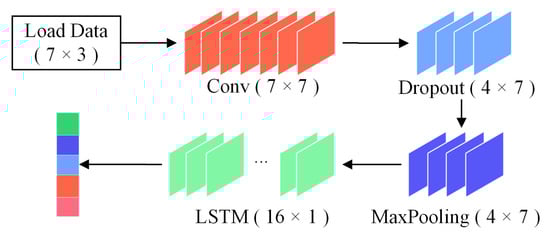
Figure 5.
The CLSTM network structure.
3.4. Environment Feature Extraction Based on LSTM
Since environmental factors have different degrees of influence on the load and the extracted environmental features are related to time series, weather data, and workday types are used as LSTM inputs, this study aims to extract features from the dimensions of the environmental factors that affect the loads by this method, thus, facilitating model learning and enhancing the generalization ability of the model. Figure 6 shows the network structure of LSTM to extract the environmental factor features. The input data are the current weather data and the type of working day. The data are input to the LSTM network consisting of 16 neurons, and finally the environmental impact features of the current moment are output.
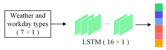
Figure 6.
The LSTM network structure.
3.5. Multidimensional Feature Fusion
It is necessary to fuse the features in a reasonable and effective way to fully take advantage of the advantages achieved on each dimensional method [28]. In this paper, we attempt to fuse multiple features by filtering, overlaying, and combining them from multidimensional features. The principle details of feature fusion are shown in Figure 7, and the Feature Confusion module part of Figure 4 shows the specific process of multidimensional feature fusion. In Figure 7, the feature fusion process is divided into two parts: one part is the splicing fusion of features, and the other part is the superposition of features.
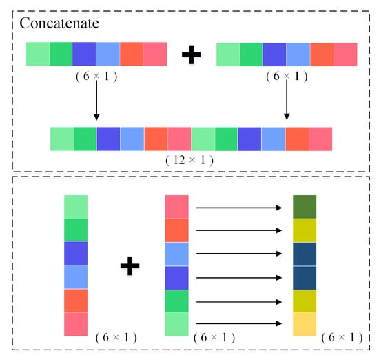
Figure 7.
The principles of feature fusion.
The splicing fusion is the first fusion of the features using a Concatenate layer for the weekly and daily feature input features, and then the first fusion of these features is done with the Dense layer based on the Softmax activate function. Secondly, the two features extracted using the AR algorithm, and the environmental factors are combined with the fused features in the first part to perform the second fusion. The fusion method uses the Add layer to superimpose the three features to complete the second feature fusion. Finally, the predicted loads are output by the Linear activate function.
4. Case Study
4.1. Case Description
The MFFCLA model was constructed and trained under the Keras and Tensorflow deep-learning frameworks on a server with two Xeon 4215R CPUs and two NVIDIA RTX 3090 GPUs. Experimental data used the integrated energy system data mentioned in Section 2. The data set is divided into training, validation, and test sets at 75%, 15%, and 10%, respectively, and the future electricity, heating, and cooling loads are predicted in 1 h steps.
4.2. Model Performance Assessment
The multi-energy load forecasting model requires prediction analysis for multiple subtasks while there are zero real load values. Therefore, the MAE (mean absolute error), and (weighted ) were selected. The MAE and indicators reflect the prediction performance of the prediction model for each load, and can reflect the performance of the model for multi-energy load forecasting as a whole, and its specific evaluation index expressions are as follows.
where , , and are the mean, true, and predicted values of the load at time t, respectively; n is the number of samples; , , and are the weights of the electricity, heating, and cooling loads, respectively; , , and are the values of the electricity, heating, and cooling loads, respectively. Considering the dominance and importance of electricity in the studied IES, and combined with the hierarchical analysis method of [29], the values of the electricity, heating, and cooling weight coefficients in Equation (5) were determined to be 0.4, 0.3, and 0.3, respectively.
4.3. Hyper-Parameter Selection
The hyper-parameter selection affects the model training effect and the actual forecasting accuracy of the model. To further explore the best model structure, the accuracy of different CNN and LSTM hyper-parameter models is compared using the control variables approach, and the appropriate optimizer is selected after the hyper-parameter combination is determined.
4.3.1. CNN LSTM Hyper-Parameter Selection
The main CNN hyper-parameters are the number of convolutional kernels, the sliding window size, and the step. The LSTM hyper-parameters are used to determine the number of LSTM units. Due to the input data structure, the sliding window size is 3, and the step is 1; therefore, only the number of convolutional kernels and the number of LSTM units need to be determined.
Figure 8 is the comparison histogram of the model prediction errors for different combinations of CNN and LSTM hyper-parameters. The number of convolutional kernel hyper-parameters of CNN and the number of neuron hyper-parameters of LSTM are [7, 14, 21] and [8, 16, 24, 32], which are combined to compare the prediction errors of the electricity, heating, and cooling loads. The CNN filters equal to 7 and LSTM units equal to 16 had the least prediction error in terms of the electricity load prediction performance, while the combination with more convolutional kernels did not perform better. Approximately the same predicted performance was found for the heating and cooling loads.
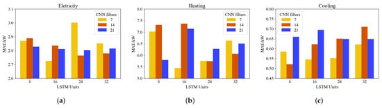
Figure 8.
Comparison of the forecasting errors for different combinations of hyper-parameters. (a) The histogram of electricity load forecasting error. (b) The histogram of electricity load forecasting error. (c) The histogram of electricity load forecasting error.
4.3.2. Optimizer Selection
As the optimization algorithms differ, their solution methods also differ, which can have some influence on the convergence and training effect of the algorithms. Therefore, in this paper, four commonly used optimizer are analyzed. Figure 9a shows the model trained with different optimizer and the forecast of the electricity, heating, and cooling loads. Among them, the prediction performance of the heating load was the most significant, while the prediction performance of the electricity and cooling loads was generally consistent. The Adam optimizer had the smallest error performance in the prediction errors of the electricity, heating, and cooling loads.
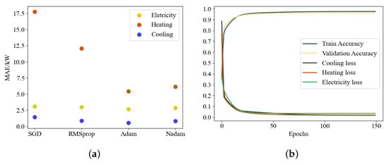
Figure 9.
Optimizer selection and model training loss performance. (a) Comparison of forecasting errors of different optimizers. (b) Loss curves and model training validation prediction accuracy curves for each load.
Figure 9b is the load loss curves of the model using the Adam optimizer and the model training/validation prediction accuracy curves. It can be seen that, when the number of training times is less than 150, the loss value of multi-energy load forecasting gradually decays, and the average accuracy of the model weights gradually increases. When the number of training times reaches 150, the loss values of multi-energy load forecasting and the average accuracy of the weights in both training and test sets converge, reflecting that the model is more similar to the actual operating data of IES when processing multi-energy load forecasting and that the model training results are credible. In summary, the specific hyper-parameters of the forecasting model are selected as shown in Table 2.
Table 2.
MFFCLA model hyper-parameter selection.
4.4. Comparison of the Proposed Model and Other Prediction Models
In order to demonstrate the practical value of the method proposed in this paper, the model MFFCLA is compared and analyzed with existing ARIMA, LSTM, and CLSTM [30].
Figure 10a,b shows the electricity and heating load, with data taken from 15 to 18 December in the winter, where the first two days are working days and the last two days are non-working days. Figure 10c shows the cooling load, with data from 29 July to 1 August in the summer, where the first two days are working days and the last two days are weekends. The forecasting results of each model used all test sets as input combined with the evaluation indexes used in this paper, and the test set prediction accuracy evaluation results are shown in Table 3 and Table 4.
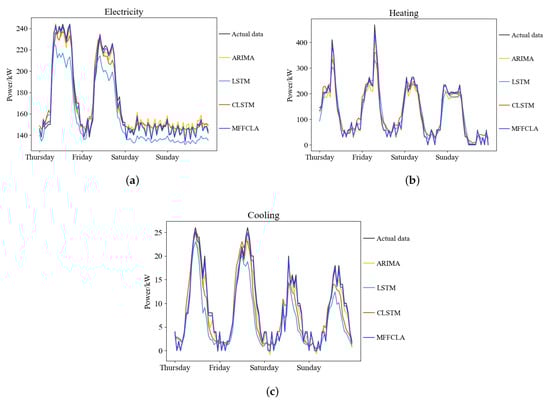
Figure 10.
Multi-energy load forecasting curves. (a) The curve of electricity load forecasting results of each model. (b) The curve of heating load forecasting results of each model. (c) The curve of cooling load forecasting results of each model.
Table 3.
evaluation.
Table 4.
MAE evaluation.
From Figure 10 as well as Table 3 and Table 4, it can be seen that all four prediction models performed well for the electricity, heating, and cooling loads. In terms of forecasting strategies, LSTM and CLSTM were more similar. Furthermore, the prediction of the three loads of CLSTM was significantly better than that of LSTM, especially in the peak performance of daily loads. It is evident that the introduction of CNN in the LSTM model can effectively extract the coupling features existing between the loads when the input data structure is the same. This further improves the forecast accuracy of the model.
The ARIMA model, which predicts the load by constructing a regression equation, also had good results. This model uses multidimensional feature fusion techniques to filter and fuse the time-series features extracted by AR, the spatial-temporal coupling features of CLSTM, and the environmental factor features of LSTM. This method organically combines the advantages of the three models to make the forecast performance more consistent with the actual load variation. MFFCLA showed excellent stability for both peak forecasts during weekday hours and smoother load forecasts during non-workday hours. This indicates that the multidimensional feature fusion technique of the model is able to fully learn the periodic characteristics present in the measured data. Therefore, this model was improved by 7.864% in the evaluation index when compared to the CLSTM model.
Figure 11 shows the red line inside the box representing the median error, the upper and lower borders of the box representing the error quartiles, the top and bottom edges representing the 1.5 times quartiles, and the dots beyond the edges representing the outliers. All four forecasting models had few anomalies, which proves that the models were stable. Four forecasting models had the largest deviation in the prediction error of the heating load, mainly due to the heating load energy demand being special. The model has difficulty learning the changing pattern of the heating load because of the large influence of climate.
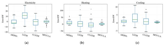
Figure 11.
Multi-energy load forecasting error box diagram. (a) The boxes of electricity load forecasting results of each model. (b) The boxes of heating load forecasting results of each model. (c) The boxes of cooling load forecasting results of each model.
The reason why the error range of the cooling load is the smallest is mainly because there is less demand for teh cooling load and less power in the building, and the value of the error deviation is also small. Secondly, the error range of the CLSTM model is smaller when compared to that of the LSTM model, and the median error line is closer to 0. This shows that the introduction of CNN structure in the CLSTM model can improve the robustness of the model and help to enhance the accuracy of the model.
As can be seen from the electricity load error box plot, the ARIMA model is based only on its trend over a short period of time when the electricity load has a periodic nature, which leads to a larger error. MFFCLA combines the advantages of CNN, LSTM, and AR from multiple dimensions by feature fusion and keeps the error range within a small range. The median line is also almost always around 0.
5. Conclusions and Discussion
In this paper, we proposed a CLSTM-AR multiple-load forecasting model based on multi-dimensional feature fusion. This model effectively combines the linear statistical ability of AR with nonlinear and periodic features extracted by LSTM and CLSTM to achieve load prediction through a multi-dimensional feature fusion method. The forecasting accuracy of MFFCLA was improved by 2.169% for ARIMA, 7.870% for CLSTMand 17.887% for LSTM. By analyzing the experimental results, the following conclusions were obtained:
By using CNN to learn the coupling relationship between energy sources, coupled with LSTM to learn the time-varying relationship among them, CLSTM effectively mined the spatial-temporal features of IES. This also considers that the load itself changes depending on the antecedent state and that AR is able to extract the state change features. In addition, considering that the environmental factors also change the energy demands, LSTM was introduced to extract the environmental impact features. Thus, comprehensive feature mining of the measurement data was achieved from multiple dimensions.
The multidimensional feature fusion method by filtering, superimposing, and combining features completes the prediction of multi-dimensional loads through linear activated layers. The process relies on backpropagation to ensure that the multidimensional features can be fused reasonably and effectively to ensure the accuracy of the model forecasting. Moreover, the fused features effectively reduce the number of model parameters, which indirectly improves the prediction efficiency of the model.
Through this study, we found that not only were energy use fluctuations at the load side influenced by weather but also different types of weekdays caused load peak variations. The load changes that occur with different weekday types can be explained to some extent as a change in the energy consumption behavior of users as describable data on the impact of the groups on the loads, including structured and unstructured data. In the future, unstructured data can be added to the method proposed in this paper to study IES multi-energy load forecasting under multi-modal data.
Author Contributions
Conceptualization, C.H., J.A. and X.L.; methodology, H.M. and B.R.; software, B.R.; validation, H.M. and B.R.; formal analysis, B.R.; investigation, H.M. and B.R.; resources, C.H., J.A. and X.L.; data curation, B.R.; writing—original draft preparation, B.R.; writing—review and editing, L.C. and H.M.; visualization, B.R.; supervision, S.M. and C.H.; project administration, H.M. and C.H.; funding acquisition, H.M. All authors have read and agreed to the published version of the manuscript.
Funding
This work was supported in part by the National Natural Science Foundation of China (No. 51907096) and in part by the Joint Fund Project of State Grid Technology Research Program (No. SGQHJY00GHJS2100269).
Data Availability Statement
All data, models, or code that support the findings of this study are available from the corresponding author upon reasonable request.
Conflicts of Interest
The authors declare no conflict of interest.
Abbreviations
The following abbreviations are used in this manuscript:
| IES | Integrated Energy System |
| CNN | Convolutional Neural Network |
| LSTM | Long Short-Term Memory Network |
| CLSTM | Convolutional Neural Network and Long Short-Term Memory Network |
| AR | Auto-Regression |
| MFFCLA | CLSTM-AR combined with Multi-Dimensional Feature Fusion |
| ARIMA | Auto-Regression Integrated Moving Average Model |
| SVM | Support Vector Machine |
| VMD | Variational Mode Decomposition |
| MTL | Multi-Task Learning |
| LSSVM | Least Square Support Vector Machine |
| DBN | Deep Belief Network |
References
- Dong, H.; Fang, Z.; Ibrahim, A.; Cai, J. Optimized Operation of Integrated Energy Microgrid with Energy Storage Based on Short-Term Load Forecasting. Electronics 2022, 11, 22. [Google Scholar]
- Gu, W.; Wang, J.; Lu, S.; Luo, Z.; Wu, C. Optimal Operation for Integrated Energy System Considering Thermal Inertia of District Heating Network and Buildings. Appl. Energy 2017, 199, 234–246. [Google Scholar] [CrossRef]
- Yan, C.; Bie, Z.; Liu, S.; Urgun, D.; Singh, C.; Xie, L. A Reliability Model for Integrated Energy System Considering Multi-Energy Correlation. J. Mod. Power Syst. Clean Energy 2021, 9, 811–825. [Google Scholar] [CrossRef]
- Boroojeni, K.G.; Amini, M.H.; Bahrami, S.; Iyengar, S.S.; Sarwat, A.I.; Karabasoglu, O. A Novel Multi-Time-Scale Modeling for Electric Power Demand Forecasting: From Short-Term to Medium-Term Horizon. Electr. Power Syst. Res. 2017, 142, 58–73. [Google Scholar] [CrossRef]
- Chen, Y.; Xu, P.; Chu, Y.; Li, W.; Wu, Y.; Ni, L.; Bao, Y.; Wang, K. Short-Term Electrical Load Forecasting Using the Support Vector Regression (SVR) Model to Calculate the Demand Response Baseline for Office Buildings. Appl. Energy 2017, 195, 659–670. [Google Scholar] [CrossRef]
- Yang, A.; Li, W.; Yang, X. Short-Term Electricity Load Forecasting Based on Feature Selection and Least Squares Support Vector Machines. Knowl.-Based Syst. 2019, 163, 159–173. [Google Scholar] [CrossRef]
- Dietrich, B.; Walther, J.; Weigold, M.; Abele, E. Machine Learning Based Very Short Term Load Forecasting of Machine Tools. Appl. Energy 2020, 276, 115440. [Google Scholar] [CrossRef]
- Ahmad, T.; Chen, H. Nonlinear Autoregressive and Random Forest Approaches to Forecasting Electricity Load for Utility Energy Management Systems. Sustain. Cities Soc. 2019, 45, 460–473. [Google Scholar] [CrossRef]
- Al-Rakhami, M.; Gumaei, A.; Alsanad, A.; Alamri, A.; Hassan, M.M. An Ensemble Learning Approach for Accurate Energy Load Prediction in Residential Buildings. IEEE Access 2019, 7, 48328–48338. [Google Scholar] [CrossRef]
- Lv, J.; Zheng, X.; Pawlak, M.; Mo, W.; Miśkowicz, M. Very Short-Term Probabilistic Wind Power Prediction Using Sparse Machine Learning and Nonparametric Density Estimation Algorithms. Renew. Energy 2021, 177, 181–192. [Google Scholar] [CrossRef]
- Bui, V.; Le, N.T.; Nguyen, V.H.; Kim, J.; Jang, Y.M. Multi-Behavior with Bottleneck Features LSTM for Load Forecasting in Building Energy Management System. Electronics 2021, 10, 1026. [Google Scholar] [CrossRef]
- Hwang, H.; Kang, S. Nonintrusive load monitoring using a lstm with feedback structure. IEEE Trans. Instrum. Meas. 2022, 71, 1–11. [Google Scholar]
- Han, M.; Zhong, J.; Sang, P.; Liao, H.; Tan, A. A Combined Model Incorporating Improved SSA and LSTM Algorithms for Short-Term Load Forecasting. Electronics 2022, 11, 1835. [Google Scholar] [CrossRef]
- Zang, H.; Xu, R.; Cheng, L.; Ding, T.; Liu, L.; Wei, Z.; Sun, G. Residential Load Forecasting Based on LSTM Fusing Self-Attention Mechanism with Pooling. Energy 2021, 229, 120682. [Google Scholar] [CrossRef]
- Wang, Y.; Gan, D.; Sun, M.; Zhang, N.; Lu, Z.; Kang, C. Probabilistic Individual Load Forecasting Using Pinball Loss Guided LSTM. Appl. Energy 2019, 235, 10–20. [Google Scholar] [CrossRef]
- Ge, L.; Li, Y.; Yan, J.; Wang, Y.; Zhang, N. Short-Term Load Prediction of Integrated Energy System with Wavelet Neural Network Model Based on Improved Particle Swarm Optimization and Chaos Optimization Algorithm. J. Mod. Power Syst. Clean Energy 2021, 9, 1490–1499. [Google Scholar] [CrossRef]
- Jin, Y.; Guo, H.; Wang, J.; Song, A. A Hybrid System Based on LSTM for Short-Term Power Load Forecasting. Energies 2020, 13, 6241. [Google Scholar] [CrossRef]
- Zhang, G.; Bai, X.; Wang, Y. Short-Time Multi-Energy Load Forecasting Method Based on CNN-Seq2Seq Model with Attention Mechanism. Mach. Learn. Appl. 2021, 5, 100064. [Google Scholar] [CrossRef]
- Ma, J.; Zhao, Z.; Yi, X.; Chen, J.; Hong, L.; Chi, E.H. Modeling Task Relationships in Multi-Task Learning with Multi-Gate Mixture-of-Experts. In Proceedings of the 24th ACM SIGKDD International Conference on Knowledge Discovery & Data Mining, New York, NY, USA, 19 July 2018; pp. 1930–1939. [Google Scholar]
- Tan, Z.; De, G.; Li, M.; Lin, H.; Yang, S.; Huang, L.; Tan, Q. Combined Electricity-Heat-Cooling-Gas Load Forecasting Model for Integrated Energy System Based on Multi-Task Learning and Least Square Support Vector Machine. J. Clean. Prod. 2020, 248, 119252. [Google Scholar] [CrossRef]
- Zhang, L.; Shi, J.; Wang, L.; Xu, C. Electricity, Heat, and Gas Load Forecasting Based on Deep Multitask Learning in Industrial-Park Integrated Energy System. Entropy 2020, 22, 1355. [Google Scholar] [CrossRef]
- Zhou, D.; Ma, S.; Hao, J.; Han, D.; Huang, D.; Yan, S.; Li, T. An Electricity Load Forecasting Model for Integrated Energy System Based on BiGAN and Transfer Learning. Energy Rep. 2020, 6, 3446–3461. [Google Scholar] [CrossRef]
- Lai, G.; Chang, W.-C.; Yang, Y.; Liu, H. Modeling Long- and Short-Term Temporal Patterns with Deep Neural Networks. In Proceedings of the 41st International ACM SIGIR Conference on Research & Development in Information Retrieval, New York, NY, USA, 27 June 2018; pp. 95–104. [Google Scholar]
- Open Energy Data Initiative (OEDI). Available online: https://data.openei.org/ (accessed on 19 September 2022).
- Denver, CO Weather History|Weather Underground. Available online: https://www.wunderground.com/history/daily/us/co/denver/KDEN/date/2011-1-1 (accessed on 19 September 2022).
- Lecun, Y.; Bottou, L.; Bengio, Y.; Haffner, P. Gradient-Based Learning Applied to Document Recognition. Proceed. IEEE 1998, 86, 2278–2324. [Google Scholar] [CrossRef]
- Hochreiter, S.; Schmidhuber, J. Long Short-Term Memory. Neural Comput. 1997, 9, 1735–1780. [Google Scholar] [CrossRef] [PubMed]
- Wang, J.; Chen, X.; Zhang, F.; Chen, F.; Xin, Y. Building Load Forecasting Using Deep Neural Network with Efficient Feature Fusion. J. Mod. Power Syst. Clean Energy 2021, 9, 160–169. [Google Scholar] [CrossRef]
- Lu, X.; Wu, J.; Hu, W.; Chi, C.; Jiang, X.; Li, X. Synthetic Evaluation of Integrated Energy System Based on AHP- Fuzzy Comprehensive Assessment Method. E3S Web Conf. 2020, 185, 01010. [Google Scholar] [CrossRef]
- Zhu, R.; Guo, W.; Gong, X. Short-Term Load Forecasting for CCHP Systems Considering the Correlation between Heating, Gas and Electrical Loads Based on Deep Learning. Energies 2019, 12, 3308. [Google Scholar] [CrossRef]


Publisher’s Note: MDPI stays neutral with regard to jurisdictional claims in published maps and institutional affiliations. |
© 2022 by the authors. Licensee MDPI, Basel, Switzerland. This article is an open access article distributed under the terms and conditions of the Creative Commons Attribution (CC BY) license (https://creativecommons.org/licenses/by/4.0/).