Detection Performance Evaluation for Marine Wireless Sensor Networks

Abstract

Detection performance evaluation is one of the inevitable problems for marine wireless sensor networks (MWSNs) deployed for target detection. However, it is a very complicated problem since it associates many different aspects, such as emitter power, range, radar cross-section, weather, geography, working mode, and so on. Targeting this problem, this paper incorporates the Poisson point process model into describing the ranges from sensors to targets. The relationship between sensors and a target is built from the perspective of detection probabilities. Then, a new consistent, conservative target detection probability evaluation is derived within a CFAR framework, and the further global detection probability of the whole MWSN on the target is developed. Additionally, the rationality of this modeling approach is demonstrated via simulation results, which is in accord with the actual situation.

1. Introduction

Recently, marine wireless sensor networks (MWSNs), composed of many sensors with the capability of wireless communication, and primary data processing floating on the sea, have been widely used in various applications, such as ocean remote sensing [1,2], maritime search and rescue [3,4], target detection (including air vessel and submarine detection) [5,6,7,8], and so on. Due to their low cost and mobile deployment, the energy budgets, communication capabilities, and the detection capabilities of the individual sensors in the MWSNs for target detection are always limited. Thus, to achieve better MWSN detection performance, detection fusion is necessary. However, it is an intractable task to fuse the individual detection performance from different sensors and consequently attain the global detection performance evaluation for the MWSNs. The reasons are two-fold. The first, as mentioned above, is that the communication capabilities of individual sensors are limited. The second is that the locations of the sensors usually change randomly because of harsh weather and rolling waves.

Most research in this area is divided into two parts. The main work focuses on the signal detection area, designed to obtain a high signal-to-noise ratio around the region of target echo signals [9,10]. However, no specific estimation of target detection probability is concerned, and the corresponding detection value is not given [11,12]. Another part concentrates on developing filters with unknown target detection probability, attempting to alleviate the dependency of the algorithm’s performance on the target detection probability. The fundamental mathematical derivation of a random finite set framework with an unknown background can be found in [13,14,15]. The influence of clutter rate on target detection probability is analyzed in [16]. Furthermore, a direct estimation of the clutter rate is incorporated into the cardinalized probability hypothesis density filter [17], and the same method is introduced in the Generalized Labeled multi-Bernoulli filter [18]. The Expectation Maximization and Markov chain Monte Carlo are used to calculate the clutter rate from real-time data at a heavy computation burden and cost [19]. Clutters are treated as a pseudo-measurement and used to jointly estimate the detection probability [20]. Nevertheless, all the research is developed on the assumption that the target detection probability is the same and the range from the sensor to the target is not considered, which does not conform to reality. In addition, the estimation of the target detection probability in a network with a random position is rarely studied.

Motivated by this, in this paper the fusion of the detection performance by different individual sensors and the evaluation of the global detection performance for the MWSNs is addressed. Specifically, we first use the Poisson point process (PPP) to characterize the spatial distribution of the individual sensors. Then, by introducing the covariance intersection (CI) algorithm, a new consistent and conservative method to evaluate the global detection performance of the MWSN is proposed. In summary, the main contributions of this paper are as follows:

First, we introduce the PPP model to describe the ranges from sensors to a target and reveal the relationship between ranges and target detection probability from the perspective of range probability;

Second, we incorporate the proposed range probability into the radar equation and achieve a target detection probability estimation through a constant false alarm rate (CFAR) detector;

Finally, we achieve a new consistent, conservative, and global detection performance evaluation for the whole MWSN by applying the CI algorithm.

The rest of the paper is organized as follows. Section 2 presents the system model and analyzes the detection performance of individual sensors. Section 3 describes the proposed method for evaluating global detection performance. Section 4 presents simulation results, followed by the conclusion in Section 5.

2. Background

To detect potential targets in a two-dimensional marine region $\Re$, we suppose that considerable wireless sensors are stochastically deployed in the region $\Re$, constituting a marine wireless sensor network (MWSN) for target detection. As shown in Figure 1, consider a target exists in this region. For convenience, the origin of the Cartesian coordinate system is set to the location of the target, and these sensors are listed as $s_1,s_2,\dots$, in increasing order, according to the distance between them with the target. Accordingly, the distance between $s_i$ and the target is denoted as $D_i$, and it follows that $D_1\le D_2\le \cdot \cdot \cdot$.

These distances are illustrated in Figure 1, and are increasingly arranged around the same target center. Similar to [21], the distribution of the number and the spatial distribution of these sensors in the MWSN are jointly modeled by a homogeneous Poisson point process (PPP) with intensity $\lambda (s)$, where $s\in {ℝ}^m$, $m\ge 1$. A realization of the PPP with intensity $\lambda (s)$, i.e., $(n,\{x_1,x_1,\dots ,x_n\})$, has the following two features [22]:

First, the number of elements in the realization, $n\ge 0$, follows the Poisson distribution with the probability mass function:

$$p(n)=\frac{{({\displaystyle {\int }_{\Re }\lambda (s)d_s})}^n}{n!}{e}^{-{\displaystyle {\int }_{\Re }\lambda (s)d_s}}$$

(1)

Second, the distribution of each element in the realization is subject to the following probability density function:

$$p(x)=\frac{\lambda (s)}{{\displaystyle {\int }_{\Re }\lambda (s)d_s}}$$

(2)

A PPP is homogeneous if there exists some constant $\alpha \ge 0$ leading to $\lambda (s)=\alpha$.

After modeling the distribution of the number and the spatial distribution of these sensors via a PPP, it is straightforward that $D_i$ is a random variable. According to [22,23], $D_i$ follows the following generalized Gamma distribution:

$$\begin{array}{cc}\hfill p_{D_i}(r)& =\frac{m{(\lambda c_m{r}^m)}^i}{r\Gamma (i)}{e}^{-\lambda c_m{r}^m}\hfill \\ & =\frac{m}{(i-1)!}{(\lambda c_m)}^i{r}^{mi-1}{e}^{-\lambda c_m{r}^m}\hfill \end{array}$$

(3)

where:

$$c_m=\frac{{\pi }^{m/2}}{\Gamma (m/2+1)}$$

(4)

and $r$ is the volume of the m-dimensional ball of radius $r$ [21]. Specifically speaking, in a two-dimensional Euclidean space, $m=2$, then we have:

$$p_{D_i}(r)=\frac{2}{(i-1)!}{(\lambda \pi )}^i{r}^{2i-1}{e}^{-\lambda \pi r^2}$$

(5)

Additionally, the expectation and variance are listed as:

$$E[D_i]=\frac{\Gamma (i/2+1)}{\sqrt{\lambda \pi }(i-1)!}$$

(6)

$$V[D_i]=\frac{n{((n-1)!)}^2-{\Gamma }^2(i+1/2)}{\lambda \pi {((n-1)!)}^2}$$

(7)

3. Methodology

For clarity, we summarize the notation used for the variables of the following part, and the corresponding meanings of those variables are given, see

Table 1. Notation of variables.

Notations	Meanings
$S_t$	emitted energy of a target
$\gamma$	loss coefficient
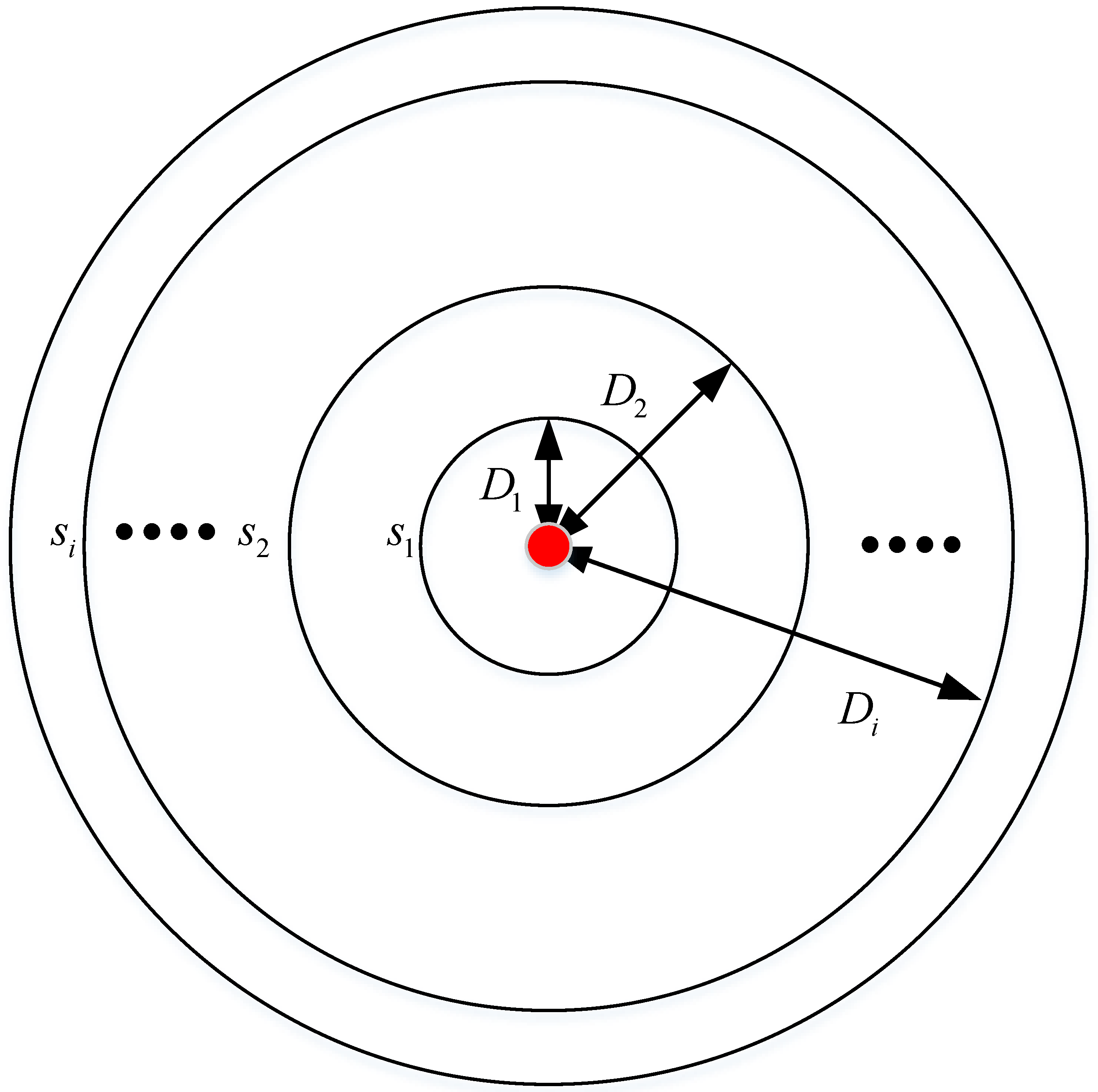
$D_i$	distance of $i$-th sensor to a target
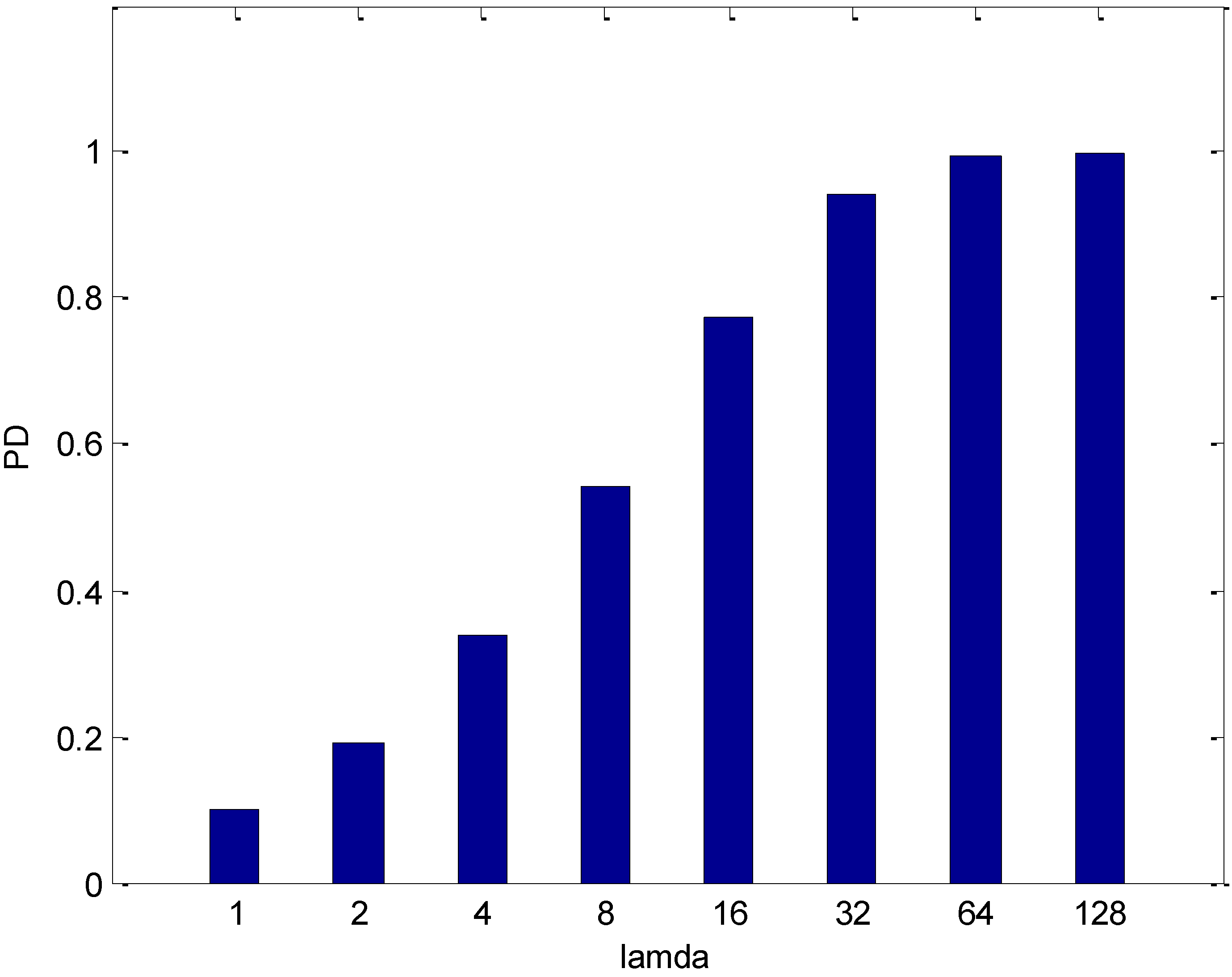
$P_D$	detection probability
$P_F$	false alarm rate
$m$	space dimension
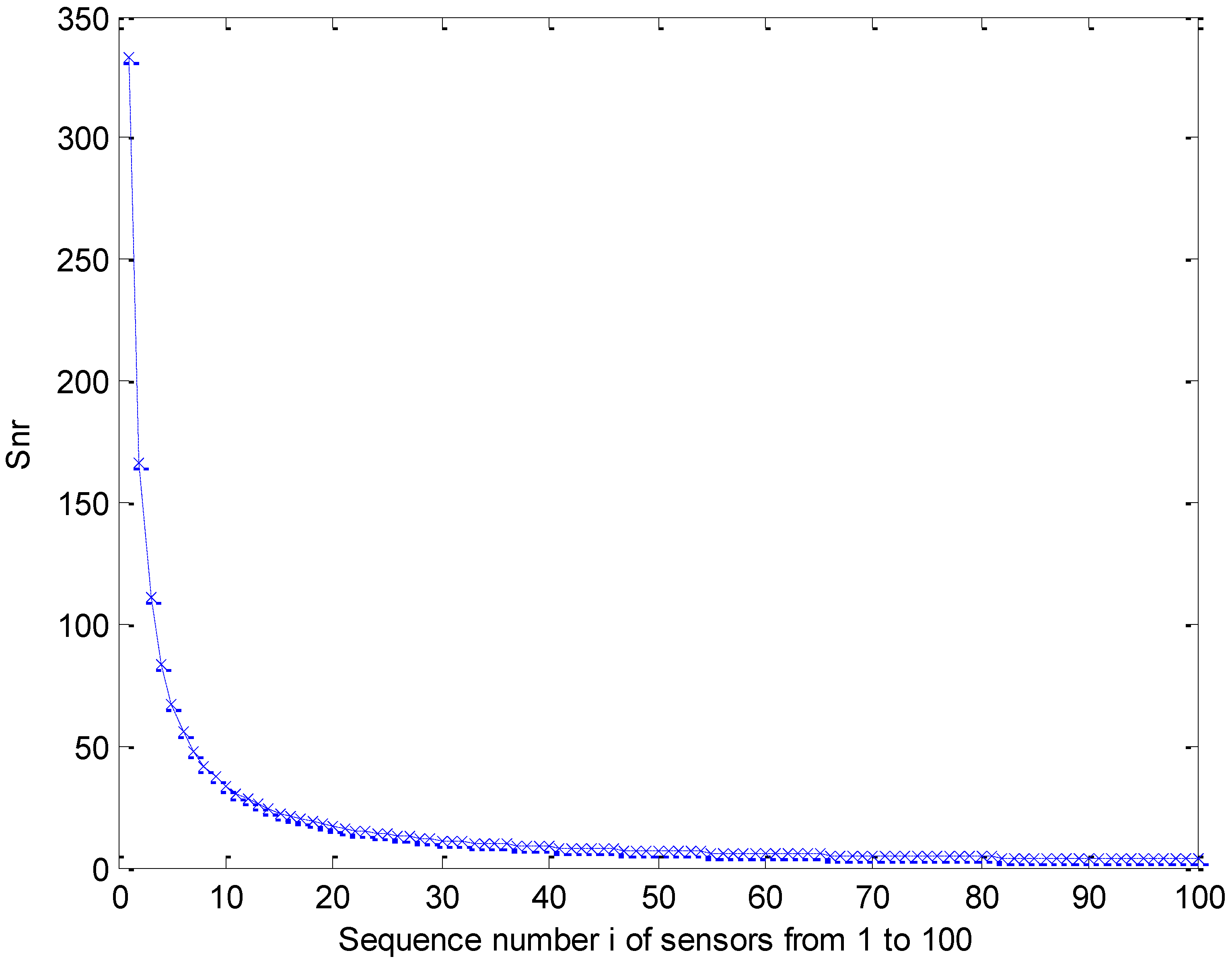
${\chi }_i$	signal-to-noise ratio
$\lambda$	Poisson intensity
${\delta }_i^2$	noise power

.

Supposing that the sensors in the MWSN detect the target by detecting the emitted energy of the target $S_t$, then the received energy at the $i$-th sensor is a function of the pate-loss coefficient $\gamma$ and the distance between the target and this sensor $D_i$ [24], and can be simplified as:

$$S_r(D_i)=\gamma \frac{S_t}{4\pi D_i^2}$$

(8)

The detection performance of each sensor is evaluated by its detection rate $P_D$ and false alarm rate $P_F$. To achieve reliable detection performance, a constant false alarm rate (CFAR) detector, which achieves maximum detection rate given a false alarm rate [11], is suggested to be adopted in each sensor. For convenience, suppose that all sensors are preset at the same given false alarm rate $P_F$. Then, the detection rate of the $i$-th sensor can be described as [25]:

$$P_{D_i}=\frac{1}{2}erfc(erf{c}^{-1}(2P_F)-\sqrt{{\chi }_i/2})$$

(9)

where $erfc(x)$ is the error compensation function defined as:

$$erfc(x)=\frac{2}{\sqrt{\pi }}{\displaystyle {\int }_x^{+00}{e}^{-t^2}dt}$$

(10)

${\chi }_i$ is the signal-to-noise ratio (SNR) at this sensor, i.e., ${\chi }_i=S_i(D_i)/{\delta }_i^2$, and ${\delta }_i^2$ is the noise power at this sensor. Substituting Equation (8) and Equation (5) into ${\chi }_i$, the expectation of SNR at the $i$-th sensor, if $m=2$, is derived as:

$$E({\chi }_i)=\frac{\gamma \lambda S_t}{4{\delta }_i^2}{\left(\frac{(i-1)!}{\Gamma (i+1)}\right)}^{-1}$$

(11)

Continuing to substitute the above equation into Equation (9), we obtain the final expression of the expectation of the detection probability:

$$E({\chi }_i)=\frac{\gamma \lambda S_t}{4{\delta }_i^2}$$

(12)

$$\sqrt{\frac{E({\chi }_i)}{2}}=\frac{\sqrt{\gamma \lambda S_t(i-1)!}}{2\sqrt{2}{\delta }_i\sqrt{\Gamma (i+1)}}$$

(13)

$$\begin{array}{ll}E(P_{D_i})& =\frac{1}{2}erfc(erf{c}^{-1}(2P_F)-\sqrt{{\chi }_i/2})\\ & \approx \frac{1}{2}erfc(erf{c}^{-1}(2P_F)-\sqrt{\frac{E({\chi }_i)}{2}})\\ & =\frac{1}{2}erfc(erf{c}^{-1}(2P_F)-\frac{\sqrt{\gamma \lambda S_t(i-1)!}}{2\sqrt{2}{\delta }_i\sqrt{\Gamma (i+1)}})\end{array}$$

(14)

It is worth noting that the second line in Equation (14) is an approximation formula because no analytic form of the integration of the Gaussian function exists. Without strictly speaking, the formula in Equation (14) is workable. Equation (14) is very meaningful since it presents the expectation of the detection probability of each sensor in these MWSNs, which can be taken as the effective index to evaluate the detection performance of each sensor. However, from the view of the party that deploys the MWSNs, a more interesting issue is the global detection performance of the MWSNs compared to that of a single sensor.

Evaluating the global detection performance of the MWSN is a challenging task. Roughly speaking, the difficulties are attributed to two reasons. The first is that the detection fusion scheme in the MWSNs is uncertain, which depends on various factors, such as communication capacities and the data processing capacities of individual sensors, while the detection fusion scheme has obvious effects on the global detection performance of the MWSNs. The second is that the confidence of the detection probabilities of individual sensors is not easy to weigh, which results in the intractable confidence of global detection performance.

In this paper, the covariance intersection (CI) algorithm presented in [26] is introduced to produce a consistent, conservative, and global detection performance evaluation for the MWSNs. As mentioned before, the detection probability of the $i$-th sensor $E(P_{D_i})$, shown in Equation (14), depends on the distance $D_i$, whose expectation $E[D_i]$ and variance $\mathrm{V}[D_i]$ are derived in Equations (6) and (7), respectively. Therefore, we suggest using $\mathrm{V}[D_i]$ to weigh the confidence of $E(P_{D_i})$ [27,28,29]. Then, inputting $E(P_{D_1})$, $E(P_{D_2})$, ⋯, and the corresponding $\mathrm{V}[D_1]$, $\mathrm{V}[D_2]$, ⋯, the global detection performance of the MWSNs via the CI algorithm is:

$$E[P_{D_f}]=(w_1{V}^{-1}[D_1]E[P_{D_1}]+w_2{V}^{-1}[D_2]E[P_{D_2}]+\cdot \cdot \cdot )V[D_f]$$

(15)

$$V[D_f]={[(w_1{V}^{-1}[D_1])+(w_2{V}^{-1}[D_2])+\cdot \cdot \cdot ]}^{-1}$$

(16)

$$1=w_1+w_2+\cdot \cdot \cdot$$

(17)

where $w_1$, $w_2$, ⋯ are fusion weights determined by minimizing the trace or determinant of $V[D_f]$. The proposed method to evaluate the global detection performance of the MWSNs consists of Equations (15)–(17). Thereinto, $E[P_{D_f}]$ is the CI-based fused detection probability, which can be taken as a consistent and conservative criterion to evaluate the global detection performance, and $V[D_f]$ is the corresponding confidence.

4. Simulation Results

Due to the space limitation, a simple radar scenario [30,31,32] is used to show the performance of the proposed method. Suppose that there is a target whose emitter power is 1000 W in the two-dimensional marine region $\Re$. The number of sensors in the MWSN is set to 100. The pate-loss coefficient is $\gamma =0.1$, the false alarm rate of a CFAR detector is set to $P_F=0.001$, $\lambda$ in a PPP process is set to 10, the dimension is $m=2$, and the power of noise at all sensors can be regarded as 1 due to simplification. Then, the evaluation results of the SNR ${\chi }_i$ and $E(P_{D_i})$ are shown in Figure 2 and Figure 3.

From Figure 2 and Figure 3, it can be seen that the SNR decreases with the increase of the range from sensor to target, which is in accord with the practical situation. The bigger sensor index means a larger range from the sensor to the target, leading to a lower target detection probability. The detection probability also deteriorates from 1 to hit 0, and the curve confirms the radar equation and the normal receiver operator characteristic (ROC) curve.

To evaluate the global detection performance of the MWSNs, the CI algorithm is used to calculate the final result. For the sake of simplicity, we use the order index to weight the corresponding $E[P_{D_1}]$, i.e.:

$$w_i=\frac{{(100-i)}^2}{{\displaystyle \sum _i{(100-i)}^2}}$$

(18)

The final evaluation result of $P_D$ is 0.7147. To test the influence of varying $\lambda$ on the detection probability $P_D$, the number of sensors is fixed at 100, and the value of $\lambda$ is ordered from 1 to 128 at an exponential rate 2. The results are shown in Figure 4.

From Figure 4, it can be seen that the larger detection probability of the whole MWSNs means the increase of parameter $\lambda$. It indicates that the expectations of distances between the sensors and the target are shorter when $\lambda$ gets larger if the number of sensors is constant in the whole network. Assuming that sensors are ordered by ascending distance to a target, the distances of the first 10 sensors to the target if $\lambda =20$ are expected to be smaller than the distances of the first 10 sensors if $\lambda =10$. This verifies the fact that the association between the distance and detection probability is positive, and the simulation results shown in Figure 4 match this fact.

5. Conclusions

Target detection probability is a key parameter in updating the step of a tracker or a filter, determining the weight between prediction results and measurements. Especially in MMWSN scenarios, the estimation of the target detection probability should take ranges from multiple sensors of the target into account, and those ranges usually are different and vary with time. To cope with this issue, this paper models the range distribution of multiple sensors in these scenarios with the target in the center using the PPP theory. The essence of this approach regards the distance between a target and a sensor as an annulus or a circle, and the probabilities of those circles of sensors are mathematically developed within the PPP framework. Based on this model, the range expectation of multiple sensors to a target is obtained. The relationship between the expected range obtained and the final target detection probability estimation is revealed in a CFAR detector. Furthermore, the CI method is introduced to calculate the global detection performance of the MWSNs, and the simulation results demonstrate the rationality of the presented method. More precisely, Figure 2 and Figure 3 show the target detection probability estimation within the range probability space, which matches the common empirical trend. The same number of sensors will be closer to the target if the parameter $\lambda$ is larger, which naturally brings a higher target detection probability.

Future work will focus on extending this modeling method of a multi-sensor target tracking framework, such as a multi-sensor random finite set filter framework or traditional probability data association framework, which will lead to interesting results. Besides, finding an analytic approximation of Equation (14) is also an interesting mathematical question, key to the mathematical integrity interpretation of this method. The Taylor expansion or Gaussian approximation are promising approaches.

References

- Luo, H.; Wang, X.; Xu, Z.; Liu, C.; Pan, J.S. A software-defined multi-modal wireless sensor network for ocean monitoring. Int. J. Distrib. Sens. Netw. 2022, 18, 1–19. [Google Scholar] [CrossRef]
- Zhou, C.; Gu, Y.; Fan, X.; Shi, Z.; Mao, G.; Zhang, Y.D. Direction-Of-Arrival estimation for coprime array via virtual array interpolation. IEEE Trans. Signal Process. 2018, 66, 5956–5971. [Google Scholar] [CrossRef]
- Wu, H.; Xian, J.; Mei, X.; Zhang, Y.; Wang, J.; Cao, J.; Mohapatra, P. Efficient target detection in maritime search and rescue wireless sensor net-work using data fusion. Comput. Commun. 2018, 136, 53–62. [Google Scholar] [CrossRef]
- Shi, C.; Ding, L.; Wang, F.; SalouASSDs, S.; Zhou, J. Joint target assignment and resource optimization framework for multitarget tracking in phased array radar network. IEEE Syst. J. 2021, 15, 4379–4390. [Google Scholar] [CrossRef]
- Fattah, S.; Gani, A.; Ahmedy, I.; Idris, M.Y.I.; Targio Hashem, I.A. A survey on underwater wireless sensor networks: Requirements, taxonomy, recent advances, and open research challenges. Sensors 2020, 20, 5393. [Google Scholar] [CrossRef]
- Diamant, R.; Lampe, L. Low probability of detection for underwater acoustic communication: A review. IEEE Access 2018, 6, 19099–19112. [Google Scholar] [CrossRef]
- Benavides, M.T.; Fodrie, F.J.; Johnston, D.W. Shark detection probability from aerial drone surveys within a temperate estuary. J. Unmanned Veh. Syst. 2019, 8, 44–56. [Google Scholar] [CrossRef]
- Yang, C.; Shi, Z.; Zhang, H.; Wu, J.; Shi, X. Multiple attacks detection in cyber-Physical systems using random finite set theory. IEEE Trans. Cybern. 2020, 50, 4066–4075. [Google Scholar] [CrossRef]
- Foglia, G.; Hao, C.P.; Farnina, A.; Giunta, G.; Orlando, D.; Hou, C. Adaptive detection of point-like targets in partially homogeneous clutter with symmetric spectrum. IEEE Trans. Aerosp. Electron. Systems. 2017, 53, 2110–2119. [Google Scholar] [CrossRef]
- Hao, C.P.; Orlando, D.; Foglia, G.; Giunta, G. Knowledge-Based adaptive detection: Joint exploitation of clutter and system symmetry properties. IEEE Signal Process. Lett. 2016, 23, 1489–1493. [Google Scholar] [CrossRef]
- Richmond, C.D. Performance of the adaptive sidelobe blanker detection algorithm in homogeneous environments. IEEE Trans. Signal Process. 2000, 48, 1235–1247. [Google Scholar] [CrossRef]
- Liu, J.; Zhou, S.; Liu, W.; Zheng, J.; Liu, H.; Li, J. Tunable adaptive detection in colocated MIMO radar. IEEE Trans. Signal Process. 2018, 66, 1080–1092. [Google Scholar] [CrossRef]
- Mahler, R. CPHD and PHD filters for unknown backgrounds, II: Multitarget filtering in dynamic clutter. Proc. SPIE 2009, 7330, 262–268. [Google Scholar]
- Mahler, R.; Elfallah, A. CPHD and PHD filters for unknown backgrounds, III: Tractable multitarget filtering in dynamic clutter. Proc. SPIE 2010, 7698, 177–188. [Google Scholar]
- Ristic, B.; Vo, B.T.; Vo, B.N.; Farina, A. A tutorial on Bernoulli filters: Theory, implementation and applications. IEEE Trans. Signal Process. 2013, 61, 3406–3430. [Google Scholar] [CrossRef]
- Mahler, R.P.S.; Vo, B.T.; Vo, B.N. CPHD filtering with unknown clutter rate and detection profile. IEEE Trans. Signal Process. 2011, 59, 3497–3513. [Google Scholar] [CrossRef]
- Beard, M.; Vo, B.T.; Vo, B.N. Multitarget filtering with unknown clutter density using a bootstrap GMCPHD filter. IEEE Signal Process. Lett. 2013, 20, 323–326. [Google Scholar] [CrossRef]
- Punchihewa, Y.G.; Vo, B.T.; Vo, B.N.; Kim, D.Y. Multiple object tracking in unknown backgrounds with labeled random finite sets. IEEE Trans. Signal Process. 2018, 66, 3040–3055. [Google Scholar] [CrossRef]
- Lian, F.; Han, C.; Liu, W. Estimating unknown clutter intensity for PHD filter. IEEE Trans. Aerosp. Electron. Syst. 2010, 46, 2066–2078. [Google Scholar] [CrossRef]
- Correa, J.; Adams, M. Estimating detection statistics within a Bayes-Closed multi-Object filter. In Proceedings of the 19th International Conference on Information Fusion (FUSION), Heidelberg, Germany, 5–8 July 2016; IEEE: Piscataway, NJ, USA, 2016; pp. 811–819. [Google Scholar]
- Dhillon, H.S.; Ganti, R.K.; Baccelli, F.; Andrews, J.G. Modeling and analysis of ktier downlink heterogeneous cellular networks. IEEE J. Sel. Areas Commun. 2012, 30, 550–560. [Google Scholar] [CrossRef]
- Streit, R.L. Poisson Point Processes: Imaging, Tracking and Sensing; Springer Science and Business Media: Berlin/Heidelberg, Germany, 2010. [Google Scholar]
- Haenggi, M. On Distances in uniformly random networks. IEEE Trans. Inf. Theory. 2005, 51, 3584–3586. [Google Scholar] [CrossRef]
- Fraiha, S.G.C.; Rodrigues, J.C.; Barbosa, R.N.S.; Gomes, H.S.; Cavalcante, G.P.S. An empirical model for propagation-Loss prediction in indoor mobile communications using the pade approximant. Microw. Opt. Technol. Lett. 2005, 48, 255–261. [Google Scholar] [CrossRef]
- Richards, M.A. Fundamentals of Radar Signal Processing; Tata McGraw-Hill Education: New York, NY, USA, 2005. [Google Scholar]
- Julier, S.; Uhlmann, J. A non-Divergent estimation algorithm in the presence of unknown correlations. In Proceedings of the 1997 American Control Conference, Albuquerque, NM, USA, 4–6 June 1997; IEEE: Piscataway, NJ, USA, 2002; pp. 2369–2373. [Google Scholar]
- Deng, Z.; Peng, Z.; Qi, W.; Liu, J.; Gao, Y. Sequential covariance intersection fusion Kalman filter. Inf. Sci. 2012, 189, 293–309. [Google Scholar] [CrossRef]
- Hurley, M.B. An information theoretic justification for covariance intersection and its generalization. In Proceedings of the IEEE International Conference on Information Fusion, Annapolis, MD, USA, 8–11 July 2002; IEEE: Piscataway, NJ, USA, 2002. [Google Scholar]
- Hu, J.; Xie, L.; Zhang, C. Diffusion Kalman Filtering Based on Covariance Intersection. IEEE Trans. Signal Process. 2011, 60, 12471–12476. [Google Scholar] [CrossRef]
- Zhang, X.; Yu, X.; Song, S.H. Outage probability and finite-SNR DMT analysis for IRS-aided MIMO systems: How large IRSs need to be? IEEE J. Sel. Top. Signal Process. 2022, 16, 1070–1085. [Google Scholar] [CrossRef]
- Shnidman, D.A. Determination of required SNR values [radar detection]. IEEE Trans. Aerosp. Electron. Syst. 2002, 38, 1059–1064. [Google Scholar] [CrossRef]
- Wang, H.; Zeng, Y. SNR scaling laws for radio sensing with extremely large-scale MIMO. In Proceedings of the IEEE International Conference on Communications Workshops (ICC Workshops), Seoul, Korea, 16–20 May 2022; IEEE: Piscataway, NJ, USA, 2022; pp. 121–126. [Google Scholar]