Fast Sidelobe Calculation for Planar Phased Arrays Using an Iterative Sidelobe Seeking Method

Abstract

Sidelobe level is a key parameter for phased array design. However, the conventional method for sidelobe level calculation is time-consuming due to the high sampling number of the radiation pattern. In this paper, an iterative sidelobe-seeking method for sidelobe calculation of arbitrarily distributed planar arrays is proposed to shorten the computing time. By applying Newton’s iterative method with an approximate formula, the proposed method uses less sampling to obtain the sidelobe positions and the peak sidelobe level. Numerical experiments were carried out and verified the effectiveness of the proposed method. Compared with the conventional method, the proposed method had a similar optimization effect but saved 80% of the algorithm time in the synthesis of a sparse planar array.

1. Introduction

Phased array is widely utilized in radar, communication and wireless power transfer applications [1,2,3]. In the design of a phased array, a lower sidelobe level (SLL) means less power loss and signal interference from undesired directions [4,5]. As a result, sidelobe calculation is applied in many problems of phased array design [6,7,8,9,10,11,12,13,14,15,16]. A number of optimization problems [6,7,8,9,10,11] take SLL calculation as the cost function directly, while others employ SLL calculation as the criterion of the scanning performance [12,13,14,17]. The SLL computing time has a direct influence on the total algorithm time in array design.

Previous studies for SLL calculation have employed two main kinds of method, the conventional method [4,6] and the fast formula method [18].

The conventional method first calculates the array pattern and then searches the sidelobe outside the main lobe region. To accurately find the sidelobe, the conventional method usually adopts a higher sampling number, which results in a longer computing time. The time complexity of the conventional method can simply be given by $O\left(mn\right)$, where m is the sampling number and n is the number of total elements. In some papers [13,14], sampling of the radiation pattern is simplified to $\phi =0$ and $\phi =\frac{\pi }{2}$ planes. Although the simplification of sampling saves computing time, the optimization results are often only effective near these two planes.

The fast formula method takes advantage of an approximate formula based on estimated sidelobe positions. This method avoids the procedure of angle sampling and, thus, has a lower time complexity, which is given as $O\left(n\right)$. However, the effectiveness of the fast formula method is sensitive to the estimated sidelobe positions. Therefore, applications of this method are limited to the optimization of the amplitudes or the phases in an array with determined element positions.

To overcome the drawbacks of previous studies, we propose an iterative sidelobe-seeking method for peak sidelobe level (PSLL) fast calculation. The proposed method considers the SLL calculation problem as a zero-finding problem of the radiation pattern derivative function. In numerical analysis, Newton’s iterative method is a fast convergent, zero-finding algorithm [19]. Combining the approximate formula in [18] with Newton’s iterative method, the proposed method adopts simple sampling of the angle domain to gradually approach the actual sidelobe positions. After comparison with the edge pattern level, the PSLL is finally obtained.

The novel features and contributions of this study can be summarized as follows,

(1) The combination of Newton’s iterative method and the approximate linear formula not only reduces the calculation pressure but also avoids the input of the estimated sidelobe positions in [18]. The linear formula facilitates the computing of second derivatives. Newton’s method removes the formula’s dependence on initial estimated sidelobe positions, which extends the application range of the formula to all kinds of array syntheses.

(2) A parallel iterative sidelobe-seeking framework is proposed to search sidelobe positions. Compared to the conventional method, the proposed framework reduces the amount of pattern sampling. Although the time complexity is still $O\left(mn\right)$, m is much smaller than that of the conventional method and, thus, computing time is saved.

The rest of this paper is organized as follows: Section 2 describes the mathematical model and algorithm details. Section 3 describes three numerical experiments undertaken to verify the proposed method. Finally, conclusions are drawn in Section 4.

2. Formulation and Algorithm

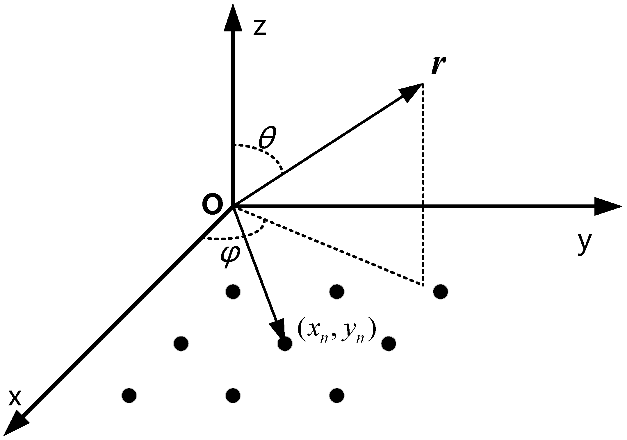
2.1. Formulation of Sidelobes in a Planar Phased Array

Figure 1 illustrates the geometry model of a planar phased array of N elements. $\theta$ and $\varphi$ are the spherical coordinate angles of a far field point $\mathbf{r}$. When the beam of the phased array is steered to the direction of $({\theta }_0,{\varphi }_0)$, the array factor could be expressed as

$$F(u,v)=\sum _n{I}_n{e}^{j[\beta (u-u_0)x_n+\beta (v-v_0)y_n+{\delta }_n]}$$

(1)

where $\beta$ is the wave number. $(x_n,y_n)$ is the position of the nth element. $I_n$ is the exciting amplitude of the nth element. ${\delta }_n$ is the phase error. $u=sin\theta cos\varphi$, $v=sin\theta sin\varphi$, $u_0=sin{\theta }_{0}cos{\varphi }_0$, $v_0=sin{\theta }_{0}sin{\varphi }_0$.

The power pattern of the array is

$$\begin{array}{cc}\hfill P(u,v)=& F\left(u,v\right)·F^{*}\left(u,v\right)\hfill \\ \hfill =& \sum _n\sum _q{I}_n{I}_q{e}^{j\left[\beta \left(u-u_0\right)\left(x_n-x_q\right)+\beta \left(v-v_0\right)\left(y_n-y_q\right)+\left({\delta }_n-{\delta }_q\right)\right]}\hfill \\ \hfill =& \sum _n\sum _q{I}_n{I}_{q}cos[\beta (u-u_0)(x_n-x_q)+\beta (v-v_0)(y_n-y_q)+{\delta }_n-{\delta }_q].\hfill \end{array}$$

(2)

where, $F^{*}(u,v)$ is the complex conjugate of $F(u,v)$.

As the sidelobes are at the extreme points of $P(u,v)$, the problem of finding the sidelobe positions involves finding the solutions of

$$\left\{\begin{array}{c}\hfill \frac{\partial P(u,v)}{\partial u}=0\\ \hfill \frac{\partial P(u,v)}{\partial v}=0\end{array}\right.$$

(3)

2.2. Newton’s Iterative Method

To obtain the roots of (3), we introduce Newton’s method of two variables. The $(k+1)$th iteration is given by

$$\begin{array}{cc}\hfill u_{(k+1)}=& u_{\left(k\right)}+\Delta u_{\left(k\right)},\hfill \\ \hfill v_{(k+1)}=& v_{\left(k\right)}+\Delta v_{\left(k\right)},\hfill \end{array}$$

(4)

where,

$$\left[\begin{array}{c}\Delta u_{\left(k\right)}\\ \Delta v_{\left(k\right)}\end{array}\right]=\left(H{(u,v)}^{-1}·\left[\begin{array}{c}-\frac{\partial P(u,v)}{\partial u}\\ -\frac{\partial P(u,v)}{\partial v}\end{array}\right]\right){|}_{u,v=u_{\left(k\right)},v_{\left(k\right)}},$$

(5)

$H(u,v)$ is the Hessian matrix of $P(u,v)$ in the form of

$$H(u,v)=\left[\begin{array}{cc}\frac{{\partial }^{2}P(u,v)}{\partial u^2}& \frac{{\partial }^{2}P(u,v)}{\partial u\partial v}\\ \frac{{\partial }^{2}P(u,v)}{\partial v\partial u}& \frac{{\partial }^{2}P(u,v)}{\partial v^2}\end{array}\right],$$

(6)

It is costly to directly use (4) due to the second derivatives in (6) and the matrix inversion in (5). Therefore, some approximation is needed. Considering that $\left(u\right(k),v(k\left)\right)$ are approaching the true extreme point $(u_m,v_m)$ after iterations, they can be used as the estimated sidelobe positions in [18] and the elements in the Hessian matrix can be approximated as,

$$\begin{array}{cc}\hfill {\displaystyle \frac{{\partial }^{2}P(u,v)}{\partial u^2}}{|}_{u,v=u_{\left(k\right)},v_{\left(k\right)}}\approx & -2{\beta }^2\{\sum _q{I}_q^c\sum _n\left[I_n^c{x}_n(x_n-O_{\mathrm{x}}^c)\right]+\sum _q{I}_q^s\sum _n\left[I_n^s{x}_n(x_n-O_{\mathrm{x}}^s)\right]\}=-2{\beta }^{2}a\hfill \\ \hfill {\displaystyle \frac{{\partial }^{2}P(u,v)}{\partial u\partial v}}{|}_{u,v=u_{\left(k\right)},v_{\left(k\right)}}\approx & -2{\beta }^2\{\sum _q{I}_q^c\sum _n\left[I_n^c{x}_n(y_n-O_{\mathrm{y}}^c)\right]+\sum _q{I}_q^s\sum _n\left[I_n^s{x}_n(y_n-O_{\mathrm{y}}^s)\right]\}=-2{\beta }^{2}b\hfill \\ \hfill {\displaystyle \frac{{\partial }^{2}P(u,v)}{\partial v^2}}{|}_{u,v=u_{\left(k\right)},v_{\left(k\right)}}\approx & -2{\beta }^2\{\sum _q{I}_q^c\sum _n\left[I_n^c{y}_n(y_n-O_{\mathrm{y}}^c)\right]+\sum _q{I}_q^s\sum _n\left[I_n^s{y}_n(y_n-O_{\mathrm{y}}^s)\right]\}=-2{\beta }^{2}d\hfill \end{array}$$

(7)

and

$$\begin{array}{cc}\hfill {\displaystyle \frac{\partial P(u,v)}{\partial u}}{|}_{u,v=u_{\left(k\right)},v_{\left(k\right)}}\approx & -2\beta \{\sum _q{I}_q^c\sum _n\left[{\delta }_n{I}_n^c(x_n-O_{\mathrm{x}}^c)\right]+\sum _q{I}_q^s\sum _n\left[{\delta }_n{I}_n^s(x_n-O_{\mathrm{x}}^s)\right]\}\hfill \\ & -2\beta \sum _q{I}_q^c\sum _n{I}_n^s(x_n-O_{\mathrm{x}}^c)=-2\beta e,\hfill \\ \hfill {\displaystyle \frac{\partial P(u,v)}{\partial v}}{|}_{u,v=u_{\left(k\right)},v_{\left(k\right)}}\approx & -2\beta \{\sum _q{I}_q^c\sum _n\left[{\delta }_n{I}_n^c(y_n-O_{\mathrm{y}}^c)\right]+\sum _q{I}_q^s\sum _n\left[{\delta }_n{I}_n^s(y_n-O_{\mathrm{y}}^s)\right]\}\hfill \\ & -2\beta \sum _q{I}_q^c\sum _n{I}_n^s(y_n-O_{\mathrm{y}}^c)=-2\beta f.\hfill \end{array}$$

(8)

where

$$\begin{array}{c}\hfill O_{\mathrm{x}}^c={\displaystyle \frac{{\sum }_q{x}_q{I}_q^c}{{\sum }_q{I}_q^c}},O_{\mathrm{y}}^c={\displaystyle \frac{{\sum }_q{y}_q{I}_q^c}{{\sum }_q{I}_q^c}},\\ \hfill O_{\mathrm{x}}^s={\displaystyle \frac{{\sum }_q{x}_q{I}_q^s}{{\sum }_q{I}_q^s}},O_{\mathrm{y}}^s={\displaystyle \frac{{\sum }_q{y}_q{I}_q^s}{{\sum }_q{I}_q^s}}\end{array}$$

(9)

and

$$\begin{array}{cc}\hfill I_n^c& =I_{n}cos(\beta \Delta u{x}_n+\beta \Delta v{y}_n),\hfill \\ \hfill I_n^s& =I_{n}sin(\beta \Delta u{x}_n+\beta \Delta v{y}_n),\hfill \\ \hfill \Delta u& =u_{\left(k\right)}-u_0,\hfill \\ \hfill \Delta v& =v_{\left(k\right)}-v_0\hfill \end{array}$$

(10)

The iterative relation (4) is converted to a linear structure as,

$$\left[\begin{array}{c}{u}_{(k+1)}-u_{\left(k\right)}\\ v_{(k+1)}-v_{\left(k\right)}\end{array}\right]\approx \frac{1}{\beta }{\left[\begin{array}{cc}a& b\\ b& d\end{array}\right]}^{-1}·\left[\begin{array}{c}-e\\ -f\end{array}\right],$$

(11)

where $a,b,d,e$ and $f$ are defined in (7) and (8).

When the condition $max\left(\right|u_{(k+1)}-u_{\left(k\right)}|,|v_{(k+1)}-v_{\left(k\right)}\left|\right)<\epsilon$ is met, the iteration is convergent. The positions of the sidelobe $u_{SL}$ and $v_{SL}$ are

$$\begin{array}{cc}\hfill u_{SL}& =u_{(k+1)}\hfill \\ \hfill v_{SL}& =v_{(k+1)}\hfill \end{array}$$

(12)

Through the Formula (1), we finally derive the sidelobe level,

$$P(u_{SL},v_{SL})={\left|F(u_{SL},v_{SL})\right|}^2.$$

(13)

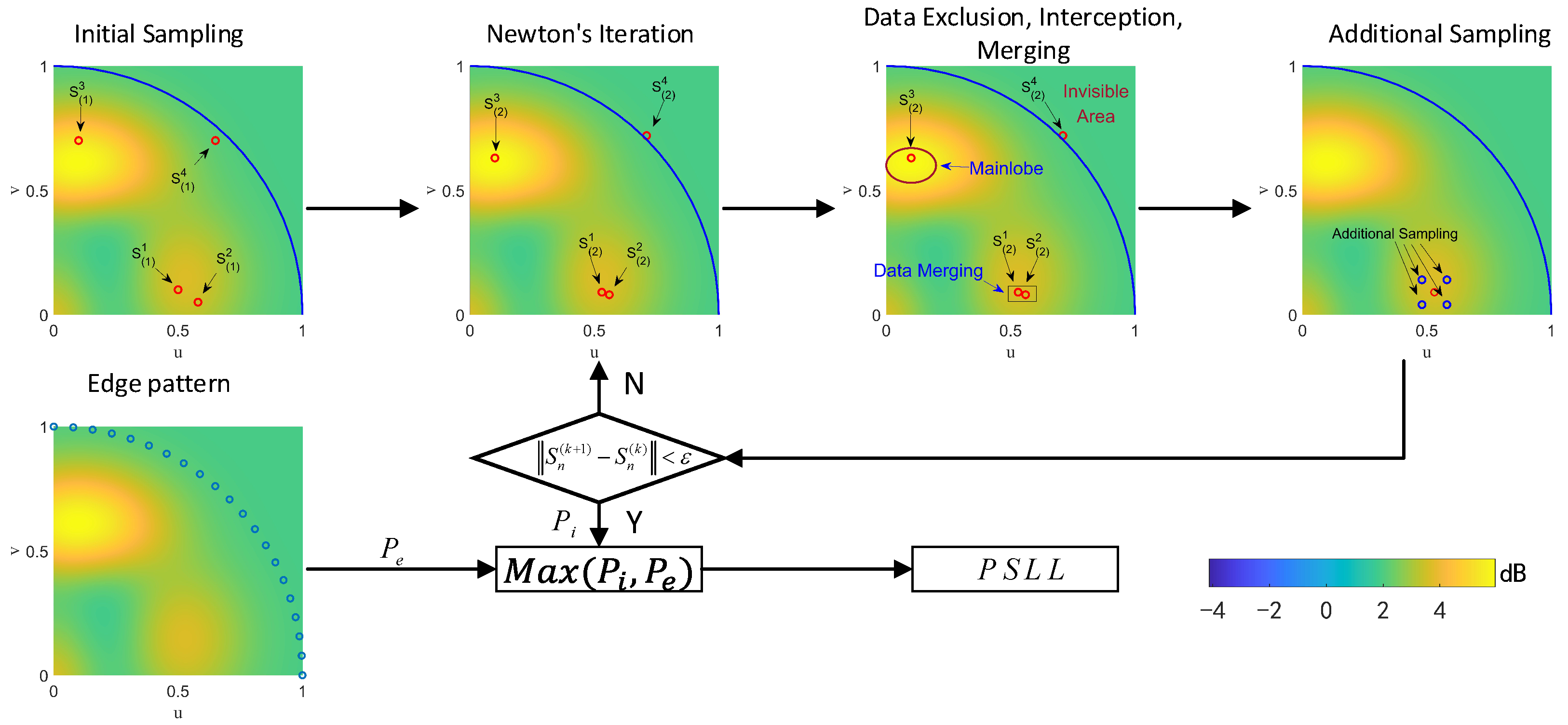
2.3. Iterative Sidelobe-Seeking Framework

Since (11) and (12) provide access to the level of a single sidelobe, we need parallel processing to approach multi-sidelobes to determine the peak sidelobe of the full pattern. Figure 2 presents the main lobe and a sidelobe in a quarter $u-v$ pattern to show the chief procedure of the proposed method. The specific details are as follows:

2.3.1. Initial Sampling

Initial sampling provides multiple inputs $(u_{\left(1\right)},v_{\left(1\right)})$ for parallel Newton iterations. The sampling methods include rectangular sampling as well as random sampling. Rectangular grid sampling is defined as,

$$\left\{\begin{array}{cc}\hfill & u_{\left(1\right)}^{ij}=-1+\frac{2(i-1)}{N_s-1},i=1,2,3\cdots ,N_s\hfill \\ & v_{\left(1\right)}^{ij}=-1+\frac{2(j-1)}{N_s-1},j=1,2,3\cdots ,N_s\hfill \\ & {\left(u_{\left(1\right)}^{ij}\right)}^2+{\left(v_{\left(1\right)}^{ij}\right)}^2\le 1\hfill \end{array}\right.$$

(14)

where $N_s$ is the sampling number of u or v dimension. The rectangular grid sampling method is also applicable to the conventional method of SLL calculation.

Random sampling adopts a uniform probability distribution for the sampling points in the $u-v$ visible area. Both sampling methods are effective here. A discussion of the methods is provided in the next section.

2.3.2. Newton’s Iteration

This step involves one iteration period using (11) for all the sampling points in parallel. We introduce (13) and calculate the power of these iterated points. For the kth iteration, we have

$$\begin{array}{cc}\hfill (u_{\left(k\right)}^1,v_{\left(k\right)}^1,& P(u_{\left(k\right)}^1,v_{\left(k\right)}^1)),\hfill \\ \hfill (u_{\left(k\right)}^2,v_{\left(k\right)}^2,& P(u_{\left(k\right)}^2,v_{\left(k\right)}^2)),\hfill \\ \hfill & ⋮,\hfill \\ \hfill (u_{\left(k\right)}^n,v_{\left(k\right)}^n,& P(u_{\left(k\right)}^n,v_{\left(k\right)}^n))\hfill \end{array}$$

(15)

2.3.3. Data Processing

After the iteration, the output points move closer to their nearest extreme points compared to their input. However, they cannot immediately be put into the next iteration before three steps of processing have occurred. The next three steps are employed to reduce the subsequent calculation.

• Data exclusion. The iterated points may move out of the visible area or into the main lobe area. These points should be excluded due to their meaninglessness for subsequent solution. The visible area conforms to $u^2+v^2\le 1$.
  The main lobe area requires an evaluation of beam width. We first calculate the pattern of the array in $u_0$-cut and $v_0$-cut as,

  $$\begin{array}{cc}\hfill P_{v_0}\left(u\right)=& P(u,v_0)={\left|F(u,v_0)\right|}^2,\hfill \\ \hfill P_{u_0}\left(v\right)=& P(u_0,v)={\left|F(u_0,v)\right|}^2.\hfill \end{array}$$

  (16)
  Secondly, the $\gamma$ dB beam width can be determined from each cut pattern. $\gamma$ is set according to the size of the array. The two beam widths are defined as ${\Gamma }_u$ and ${\Gamma }_v$. As the main lobe is approximately elliptical in the $u-v$ system, the area is marked as,

  $${\left(\frac{u-u_0}{\frac{1}{2}{\Gamma }_u}\right)}^2+{\left(\frac{v-v_0}{\frac{1}{2}{\Gamma }_v}\right)}^2\le 1$$

  (17)
• Data interception. This step cuts off the iterated points with low power due to their low possibility of iterating to the extreme points. The criteria for the interception are a certain proportion of the total points or a certain power value.
• Data merging. This step merges the close points into one point. If two points $(u_a,v_a)$ and $(u_b,v_b)$ meet the condition ${(u_a-u_b)}^2+{(v_a-v_b)}^2<L$, they are to be merged. L is a preset parameter.

2.3.4. Additional Sampling

The initial sampling may not cover all the sidelobes. Therefore, this step adds extra sampling around the points of the higher power. In our programming, the extra samplings $(u_e,v_e)$ for a single sampling point $(u_{\left(k\right)},v_{\left(k\right)})$ can be expressed as,

$$\begin{array}{cc}\hfill u_e^{\left(i\right)}& =u_{\left(k\right)}+R_{e}cos\left[\alpha \left(i\right)\right]\hfill \\ \hfill v_e^{\left(i\right)}& =v_{\left(k\right)}+R_{e}sin\left[\alpha \left(i\right)\right]\hfill \end{array}$$

(18)

where, $\alpha \left(i\right)=\left(i-1\right)2\pi /N_e$, and $N_e$ is a user-defined parameter. $R_e$ reflects the precision of the radiation pattern and is usually evaluated by ${\Gamma }_u$ and ${\Gamma }_v$ as,

$$R_e=max({\Gamma }_u,{\Gamma }_v).$$

(19)

2.3.5. Iteration and the Iteration End

Repeat the steps from (2) to (6) until the convergent condition $max\left(\right|u_{(k+1)}^n-u_{\left(k\right)}^n|,|v_{(k+1)}^n-v_{\left(k\right)}^n\left|\right)<\epsilon$ is met. After the iterations are ended, we acquire a series of points sorted by their powers. The maximum power $P_i$ is a candidate for the final result, which can be expressed as,

$$P_i=max[P(u_{(k+1)}^1,v_{(k+1)}^1),P(u_{(k+1)}^2,v_{(k+1)}^2),\cdots ,P(u_{(k+1)}^n,v_{(k+1)}^n)].$$

(20)

2.3.6. Edge Pattern

The sidelobes may appear at the extreme points of $P(u,v)$ as well as at the edge of the visible area. The side lobes on the edge of the visible area may not be caught by the iterations. To solve this problem, we need to calculate the array pattern of the edge area (${\left(u_{edge}^n\right)}^2+{\left(v_{edge}^n\right)}^2=1$) and obtain $P_e$ as,

$$P_e=max[P(u_{edge}^1,v_{edge}^1),P(u_{edge}^2,v_{edge}^2),\cdots ,P(u_{edge}^n,v_{edge}^n)].$$

(21)

2.3.7. Final Result

The peak sidelobe level can be expressed as $\mathrm{PSLL}=max({\mathrm{P}}_{\mathrm{i}},{\mathrm{P}}_{\mathrm{e}})$.

2.4. Analysis of Computational Complexity

Due to the linear structure of (11), the time computational complexity of the iterative sidelobe-seeking method is $O\left(N{n}_{s_1}^2\right)$, where N is the total element number and $n_{s_1}$ is the sampling number in (14).

The conventional method of SLL calculation usually contains three steps:

• Sampling the $u-v$ area. Usually, the sampling method for the conventional method is rectangular sampling, which can take the form of (14).
• Computing the array factor of the sampling points using (1) and forming the array pattern.
• Searching and determining the peak sidelobe among the array pattern.

When the sampling number is $n_{s_2}$, the conventional time computational complexity is $O\left(N{n}_{s_2}^2\right)$. For larger arrays, $n_{s_2}$ is at least 200, while $n_{s_1}$ only needs to be 50 or less. Therefore, the proposed method can systematically reduce the SLL calculation time.

3. Numeric Experiments and Results

This section describes numeric experiments performed to verify the effectiveness of the iterative sidelobe-seeking method in the PSLL calculation. The computing procedure was mainly performed in MATLAB on a computer equipped with a CPU of 3.0 GHz and RAM of 8 GB.

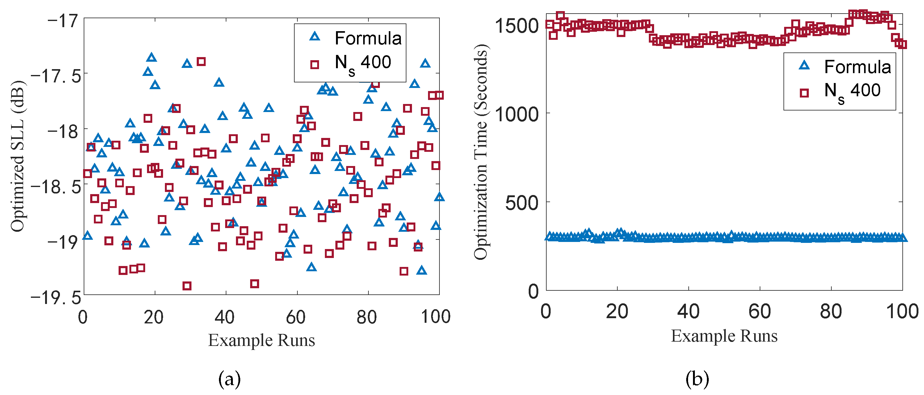
3.1. Sidelobe Calculation for Square Aperture Arrays

This example involved checking the performance of the iterative sidelobe-seeking method in the case of large planar arrays with elements of 400, 900, 1600, and 2500. The array element positions were generated based on $20\times 20$, $30\times 30$, $40\times 40$ and $50\times 50$ uniform arrays with an element distance of 0.5 wavelength ($\lambda$) (the circles in a light color in Figure 3a). The example was conducted for 100 runs. To increase the complexity of our example, the array element positions in both x and y directions involved random variation of $\pm 0.3$ $\lambda$ in each run (the circles in a dark color in Figure 3a). Figure 3b is a sample of the array element distribution. The amplitude of each element conformed to $U(0,1)$. The phase shifter bit value was 3. The errors of the phase were ${\delta }_n\sim U(0,\frac{\pi }{4})$. In addition, the beam point angles were also random, where ${\theta }_0\sim U(0,\frac{\pi }{3})$ and ${\varphi }_0\sim U(0,2\pi )$.

For the proposed method, we used rectangular sampling and set $N_s$ as 44, 46, 48, and 50 to study the effect on performance. $\gamma$ was set to 17. L was set to 0.1 (we tried a series of L values and 0.1 showed the best performance). When the number of iterations was four, the iterations were considered to be convergent. As a comparison, we also applied the conventional method using the sampling strategy of (14). Three kinds of sampling numbers, 200, 400, and 1000 were adopted. We considered the result of the sampling number of 1000 to be the accurate value. We also applied the fast method in [18] for comparison.

The results are provided in

Table 1. Comparison of sidelobe absolute errors (dB) with different methods.

Array Size	400	900	1600	2500
Proposed ($N_s$ 44)	0.013	0.022	0.064	0.052
Proposed ($N_s$ 46)	0.003	0.022	0.035	0.046
Proposed ($N_s$ 48)	0.002	0.016	0.023	0.049
Proposed ($N_s$ 50)	0.001	0.012	0.010	0.035
Conventional ($N_s$ 400)	0.009	0.023	0.040	0.061
Conventional ($N_s$ 200)	0.045	0.089	0.167	0.189
Fast method in [18]	0.003	0.033	0.039	0.061

and

Table 2. Comparison of computing time (s) with different methods.

Array Size	400	900	1600	2500
Proposed ($N_s$ 44)	0.124	0.164	0.257	0.368
Proposed ($N_s$ 46)	0.130	0.189	0.271	0.385
Proposed ($N_s$ 48)	0.144	0.202	0.285	0.405
Proposed ($N_s$ 50)	0.147	0.216	0.307	0.457
Conventional ($N_s$ 400)	1.106	1.824	2.850	4.184
Conventional ($N_s$ 200)	0.277	0.459	0.718	1.050
Fast method in [18]	0.283	0.462	0.709	1.100

. The sampling numbers for the proposed method had a direct influence on both the accuracy and the computing time. As the sampling numbers ($N_s$) increased, the average errors decreased and the computing time increased. For a desired accuracy, the array with more elements required a higher sampling number. In addition, the computing time increased along with the number of array elements.

The iterative sidelobe-seeking method had an advantage over the conventional method. The proposed method with $N_s$ of 50 obtained better accuracy than the conventional method of 400-sampling, but only consumed 11% computing time in the array of 2500 elements. When compared to the conventional method of 200-sampling, the proposed method resulted in an 18% average error and consumed 42% computing time.

The proposed method performed better than the method described in [18]. Although the method in [18] exhibited good accuracy, the computing time was similar to that of the conventional method of 200-sampling. This was because the input estimated sidelobe positions were calculated by the conventional method of 200-sampling.

Finally, we also compared the performance between rectangular sampling and random sampling in the array of 1600 elements. As shown in

Table 3. Performance of Different Sampling Methods.

Sampling Type	Sampling Number	Mean Error (dB)	Time (s)
Random	2049	0.0188	0.3094
Random	1984	0.0214	0.3006
Random	1746	0.0311	0.2725
Random	1596	0.0397	0.2610
Random	1442	0.0483	0.2516
Rectangular	1961 ($N_s$ 50)	0.0095	0.3061
Rectangular	1793 ($N_s$ 48)	0.0231	0.2835
Rectangular	1576 ($N_s$ 46)	0.0265	0.2707

, the rectangular sampling of 1961 produced the best result among all the experiments. In addition, the experiments in which there was a small number of samples consumed less computing time, which means that random sampling provided no advantage for improving efficiency.

3.2. Sidelobe Calculation for Circular Array with Taylor Weighting

To verify the effectiveness of the iterative sidelobe-seeking method with a larger amplitude of variation, this example considered a Taylor-weighted circular array with an aperture size of 12 $\lambda$. The array adopted a rectangular grid with 0.5 $\lambda$. The total element number was 448. The example was also conducted for 100 runs. Complying with the Taylor distribution of −30 dB, the amplitude of each element had a random error of 30%. Except for the amplitude, the array element positions, the phase errors, and the beam point angles all exhibited random variations similar to the first example. Figure 4a shows a random sample of the array distribution.

In this example, $\gamma$ was set to 30 to meet the more drastic sidelobe level change. Similarly, the conventional method of $N_s$-1000 sampling was responsible for the accurate value.

Figure 4b and Figure 5 are the results of the proposed method comparing the $N_s$-200 and $N_s$-400 samplings. The iterative sidelobe-seeking method is represented as ’Proposed’. Figure 5a shows the absolute errors of each method compared to the accurate value. To better analyze the error distribution, Figure 5b shows the boxplot graph for the three methods. The statistical results indicate that our formula was more accurate than $N_s$-200 and close to the $N_s$-400. As shown in Figure 4b, the proposed method saved 54% and 89% algorithm time compared to the $N_s$-200 and $N_s$-400 samplings.

Based on the above two examples, a comparison between previous studies and the proposed method is presented in

Table 4. The comparison of the proposed method with other methods.

	Conventional Method	Fast Formula Method	Proposed Method
Time Complexity	O (mn)	O (n)	O (mn)
Computing Time	slow	fast	middle
Scope of Application	any planar arrays	planar arrays with given positions	any planar arrays
Accuracy	high	middle	high

.

3.3. Synthesis of Sparse Planar Arrays

In this experiment, we applied the iterative sidelobe-seeking method in the synthesis of sparse planar arrays using the modified real genetic algorithm [6]. The array aperture was symmetrical in a rectangle of $9.5\lambda \times 4.5\lambda$. The minimum element spacing was 0.5 $\lambda$. The number of sparse elements was 100. The fitness function was the PSLL. We used the proposed method and the conventional method in the calculations of fitness for comparison. $\gamma$ was 15 in the proposed method. $N_s$ was 400 in the conventional method. Each method was conducted for 100 runs. In the genetic algorithm, both the generation number and the population size were 100.

Figure 6 presents the results of the two methods. As shown in Figure 6a, the average SLL of the proposed method was −18.31 dB, while the average SLL of the conventional method was −18.50 dB. The two methods produced similar results. As shown in Figure 6b, our method consumed only 20.1% of the computing time of the conventional method. In general, by replacing the conventional method with the proposed method, we were able to achieve similar results with less time in practical applications.

4. Conclusions

In this paper, an iterative sidelobe-seeking method for PSLL calculation was proposed for planar phased arrays involving converting SLL calculation to the zero-point problem of a radiation pattern derivative function. Applying Newton’s iterations, the proposed method approximates the simple sampling positions to the actual sidelobe positions, which reduces the sampling number of the pattern and overcomes the need for initial estimation. The peak sidelobe position and level are obtained after the processing of an iterative sidelobe-seeking framework. The proposed method was verified using numerical examples and possessed better accuracy and efficiency in comparison with conventional methods and the fast method described in [18]. In addition, we tested the performance of the proposed method in practical applications. With the effect of optimization, the proposed method was able to save 80% algorithm time in the synthesis of a sparse planar array. The proposed method is applicable not only for phased arrays but also for all kinds of planar arrays, and, thus, could improve the efficiency of array design for radar and communication.

References

1. Brookner, E. Advances and breakthroughs in radars and phased-arrays. In Proceedings of the 2016 CIE International Conference on Radar (RADAR), Guangzhou, China, 10–13 October 2016; pp. 1–9. [Google Scholar] [CrossRef]
2. Warnick, K.F.; Maaskant, R.; Ivashina, M.V.; Davidson, D.B.; Jeffs, B.D. Phased Arrays for Radio Astronomy, Remote Sensing, and Satellite Communications; Cambridge University Press: Cambridge, UK, 2018. [Google Scholar]
3. Lopezf, J.; Tsay, J.; Guzman, B.; Mayeda, J.; Lie, D. Phased arrays in wireless power transfer. In Proceedings of the 2017 IEEE 60th International Midwest Symposium on Circuits and Systems (MWSCAS), Boston, MA, USA, 6–9 August 2017; pp. 5–8. [Google Scholar] [CrossRef]
4. Mailloux, R.J. Phased Array Antenna Handbook, 3rd ed.; Artech House: Norwood, MA, USA, 2018. [Google Scholar]
5. Balanis, C.A. Antenna Theory: Analysis and Design, 4th ed.; Wiley: Hoboken, NJ, USA, 2015. [Google Scholar]
6. Chen, K.; Yun, X.; He, Z.; Han, C. Synthesis of Sparse Planar Arrays Using Modified Real Genetic Algorithm. IEEE Trans. Antennas Propagat. 2007, 55, 1067–1073. [Google Scholar] [CrossRef]
7. Rocha-Alicano, C.; Covarrubias-Rosales, D.; Brizuela-Rodriguez, C.; Panduro-Mendoza, M. Differential evolution algorithm applied to sidelobe level reduction on a planar array. AEU-Int. J. Electron. Commun. 2007, 61, 286–290. [Google Scholar] [CrossRef]
8. Cen, L.; Yu, Z.L.; Ser, W.; Cen, W. Linear Aperiodic Array Synthesis Using an Improved Genetic Algorithm. IEEE Trans. Antennas Propagat. 2012, 60, 895–902. [Google Scholar] [CrossRef]
9. Pappula, L.; Ghosh, D. Linear Antenna Array Synthesis using Cat Swarm Optimization. AEU-Int. J. Electron. Commun. 2014, 68, 540–549. [Google Scholar] [CrossRef]
10. Liu, H.; Zhao, H.; Li, W.; Liu, B. Synthesis of Sparse Planar Arrays Using Matrix Mapping and Differential Evolution. IEEE Antennas Wirel. Propagat. Lett. 2016, 15, 1905–1908. [Google Scholar] [CrossRef]
11. Pinchera, D.; Migliore, M.D.; Panariello, G. Synthesis of Large Sparse Arrays Using IDEA (Inflating-Deflating Exploration Algorithm). IEEE Trans. Antennas Propagat. 2018, 66, 4658–4668. [Google Scholar] [CrossRef]
12. Anselmi, N.; Rocca, P.; Salucci, M.; Massa, A. Irregular Phased Array Tiling by Means of Analytic Schemata-Driven Optimization. IEEE Trans. Antennas Propagat. 2017, 65, 4495–4510. [Google Scholar] [CrossRef]
13. Dong, W.; Xu, Z.H.; Liu, X.; Wang, L.; Xiao, S.P. Modular Subarrayed Phased Array Design by Means of Iterative Convex Relaxation Optimization. IEEE Antennas Wirel. Propagat. Lett. 2019, 18, 447–451. [Google Scholar] [CrossRef]
14. Yang, K.; Wang, Y.; Tang, H. A Subarray Design Method for Low Sidelobe Levels. Prog. Electromagn. Res. Lett. 2020, 89, 45–51. [Google Scholar] [CrossRef] [Green Version]
15. Hwang, Y.; Han, C. The use of GTD in the design and analysis of low sidelobe reflector antennas. Proc. Antennas Propag. Soc. Int. Symp. 1981, 19, 484–487. [Google Scholar] [CrossRef]
16. Odendaal, J.; Pistorius, C. Horn Antenna with Suppressed Sidelobe Level. Microw. Opt. Technol. Lett. 1991, 4, 238–239. [Google Scholar] [CrossRef]
17. Rocca, P.; Mailloux, R.J.; Toso, G. GA-Based Optimization of Irregular Subarray Layouts for Wideband Phased Arrays Design. IEEE Antennas Wirel. Propagat. Lett. 2015, 14, 131–134. [Google Scholar] [CrossRef]
18. Miao, K.; Zhang, Y.; Sun, H. Fast Sidelobe Calculation and Suppression in Arbitrary Two-Dimensional Phased Arrays. IEEE Antennas Wirel. Propagat. Lett. 2021, 20, 928–932. [Google Scholar] [CrossRef]
19. Sauer, T. Numerical Analysis; Pearson Education: Boston, MA, USA, 2011. [Google Scholar]
Figure 1. A planar phased array consisting of N elements positioned on the x y -plane.
Electronics 11 03366 g001
Figure 2. The procedure of peak sidelobe seeking ( S ( n ) m is the mth sampling point of the nth iteration).
Electronics 11 03366 g002
Figure 3. Generation and example of array distribution in the numeric experiments. (a) The generation of the random positions of the array. (b) A sample distribution of an array of 1600 elements.
Electronics 11 03366 g003
Figure 4. (a) A sample distribution of array elements for Section 3.2. (b) Computing time comparison of example Section 3.2.
Electronics 11 03366 g004
Figure 5. Error performance of example Section 3.2. (a) Absolute error analysis. (b) Boxplot of errors.
Electronics 11 03366 g005
Figure 6. Comparison of the two methods in the synthesis of sparse arrays. (a) Comparison of optimized SLLs. (b) Comparison of optimization time.
Electronics 11 03366 g006