A Study on the Stability of Graph Edit Distance Heuristics

Abstract

Graph edit distance (GED) is a powerful tool to model the dissimilarity between graphs. However, evaluating the exact GED is NP-hard. To tackle this problem, estimation methods of GED were introduced, e.g., bipartite and IPFP, during which heuristics were employed. The stochastic nature of these methods induces the stability issue. In this paper, we propose the first formal study of stability of GED heuristics, starting with defining a measure of these (in)stabilities, namely the relative error. Then, the effects of two critical factors on stability are examined, namely, the number of solutions and the ratio between edit costs. The ratios are computed on five datasets of various properties. General suggestions are provided to properly choose these factors, which can reduce the relative error by more than an order of magnitude. Finally, we verify the relevance of stability to predict performance of GED heuristics, by taking advantage of an edit cost learning algorithm to optimize the performance and the k-nearest neighbor regression for prediction. Experiments show that the optimized costs correspond to much higher ratios and an order of magnitude lower relative errors than the expert cost.

1. Introduction

Graphs provide a flexible representation framework to encode elements as well as the relationships between them, enabling to capture the underlying structural information of the data. Despite providing rich expressiveness, the complexity lying in graph structures becomes its Achilles’ heel when applying machine learning methods for graph data, which are mainly designed to operate on vector representations [1,2]. To leverage this flaw, several approaches have been designed to learn models on graphs, representatives among which include graph embedding strategy [3], graph kernels [4,5], and more recently graph neural networks [6], some of which are closely connected with signal processing on graphs [7,8,9,10,11,12]. Despite their state-of-the-art performances, they seldom operate directly in a graph space, hence reducing the interpretability of the underlying operations. To overcome these issues and preserve the properties of a graph space, some (dis)similarity measure or metric is usually assigned to that space, since most machine learning algorithms rely on (dis)similarity measures between data. One of the most used dissimilarity measures between graphs is the graph edit distance (GED) [13,14]. The GED of two graphs $G_1$ and $G_2$ is the minimal amount of distortion required to transform $G_1$ into $G_2$. 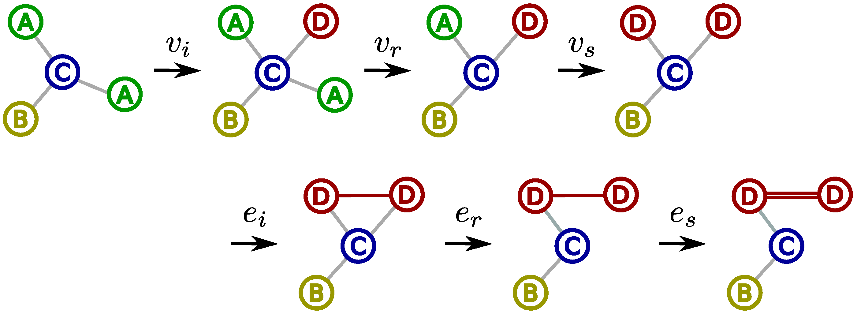This transformation includes a series of six elementary edit operations, namely vertex and edge substitutions ($v_s$ and $e_s$), removals ($v_r$ and $e_r$), and insertions ($v_i$ and $e_i$), as shown in  Figure 1. This sequence of edit operations constitutes an edit path $\pi$. A non-negative cost $c\left(e\right)$ can be assigned to each edit operation e. The sum of all edit operation costs included within $\pi$ is defined as the cost associated with $\pi$. The minimal cost among all edit paths defines the GED between $G_1$ and $G_2$.

Evaluating exact GED is NP-hard even for uniform edit costs [15]. In practice, it cannot be done for graphs having more than 12 vertices in general [16]. To avoid this computational burden, strategies to approximate GED in a limited computational time have been proposed [17,18] with acceptable classification or regression performances. Of particular interest are the two famous methods, bipartite [19] and IPFP [20], where upper and lower bounds are estimated as an approximation of GED. The computation of the bounds relies highly on the design of the algorithm, as well as the randomness during the procedure, which leads to a reduction of stability.

As this paper will illustrate, the stability of the GED heuristics is highly relevant to the choice of heuristic method and their prediction performance. As GED is a widely used similarity between graphs, the study of stability can be useful to help promote the performance of GED in various tasks.

In this paper, it is the first time that the stability of GED heuristics has been formally studied. We define the instability of a GED heuristic in terms of the variability of the GED approximations over repeated trials. Methods that can potentially alleviate this problem are proposed. For instance, by carrying out several local searches in parallel, the multi-start counterparts of bipartite and IPFP, named mbipartite and mIPFP, respectively, may acquire better approximation with higher stability [21]. Description and analyses of these approximations and the root of randomness are presented in Section 3 and Section 4.

Another essential ingredient of GED is the underlying edit cost function $c\left(e\right)$, which quantifies the distortion carried by any edit operation e. The values of the edit costs for each edit operation have a major impact on the computation of GED and its performance, including its stability [17,22]. Besides fixing costs provided a priori by domain experts for a given dataset, methods are proposed to optimize these costs, e.g., by aligning metrics in the graph to target spaces [23]. Analyzing the optimized edit costs helps further explore its relevance to the stability of GED heuristics.

The remaining part of the paper is organized as follows: Section 2 introduces widely used GED heuristics paradigms. Section 3 defines a measure of the (in)stability of these heuristics, as well as two factors of critical influence. Then, Section 4 gives experiments and analyses. Finally, Section 5 concludes the work and open perspectives.

2. Graph Edit Distances Heuristics

Over the years, many heuristics have been proposed to approximate GED. The authors of [18] categorize these heuristics according to their underlying paradigms. As milestones and baselines to many other heuristics, both bipartite and IPFP achieve high performance [17]. Thereby, in the following sections, we focus on these two heuristics and the related paradigms. First, we provide preliminary definitions of graphs and graph edit distances.

2.1. Graphs and Graph Edit Distances

A graph $G=(V,E)$ is an ordered pair of disjoint sets, where V is the vertex set and $E\in V\times V$ is the edge set. A graph can have a label set L from a label space and a labeling function ℓ that assigns a label $l\in L$ to each vertex and/or edge.

Given a set $\mathcal{G}$ of N graphs, the Graph Edit Distance (GED) between two graphs $G_i$ and $G_j$$\in \mathcal{G}$ is defined as the cost of minimal transformation [19]:

$$\mathtt{ged}(G_i,G_j)=\underset{\pi \in \mathsf{\Pi }(G_i,G_j)}{min}C(\pi ,G_i,G_j),$$

(1)

where $\pi (G_i,G_j)$ is a mapping between $V_i\cup \epsilon$ and $V_j\cup \epsilon$ encoding the transformation from $G_i$ to $G_j$, and $\epsilon$ represents a dummy element [20]. As described in Section 1, this transformation consists of a series of six elementary operations: removing or inserting a vertex or an edge, and substituting a label of a vertex or an edge by another. $C(\pi ,G_i,G_j)$ measures the cost associated with $\pi$:

$$\begin{array}{cc}\hfill & C(\pi ,G_i,G_j)=\sum _{\begin{array}{c}v\in V_j\\ {\pi }^{-1}\left(v\right)=\epsilon \end{array}}{c}_{vfi}+\sum _{\begin{array}{c}v\in V_i\\ \pi \left(v\right)=\epsilon \end{array}}{c}_{vfr}+\sum _{\begin{array}{c}v\in V_i\\ \pi \left(v\right)\ne \epsilon \end{array}}{c}_{vfs}\hfill \\ \hfill & +\sum _{\begin{array}{c}e=(v_i,v_j)\in E_j|\\ {\pi }^{-1}\left(v_i\right)=\epsilon \vee \\ {\pi }^{-1}\left(v_j\right)=\epsilon \vee \\ ({\pi }^{-1}\left(v_i\right),{\pi }^{-1}\left(v_j\right))\notin E_i\end{array}}{c}_{efi}+\sum _{\begin{array}{c}e=(v_i,v_j)\in E_i|\\ \pi \left(v_i\right)=\epsilon \vee \\ \pi \left(v_j\right)=\epsilon \vee \\ (\pi \left(v_i\right),\pi \left(v_j\right))\notin E_j\end{array}}{c}_{efr}+\sum _{\begin{array}{c}e=(v_i,v_j)\in E_i|\\ \pi \left(v_i\right)\ne \epsilon \wedge \\ \pi \left(v_j\right)\ne \epsilon \wedge \\ (\pi \left(v_i\right),\pi \left(v_j\right))\in E_j\end{array}}{c}_{efs},\hfill \end{array}$$

(2)

where $c_{vfr},c_{vfi},c_{vfs},c_{efr},c_{efi},c_{efs}$ are the edit costs associated with the six edit operations: respectively, vertex removal, insertion, substitution and edge removal, insertion, and substitution. Without loss of generality, these costs are set to be constant for each edit operation in the following part, denoted, respectively, as $c_{vr},c_{vi},c_{vs},c_{er},c_{ei},c_{es}$.

2.2. Paradigm LSAPE-GED and Heuristic Bipartite

GED can be approximated by solving a linear sum assignment problem with edition or error correction (LSAPE). For any two sets $V_1$ and $V_2$, consider a transformation from $V_1$ to $V_2$, with elementary operations on each element $i\in V_1$: substitution ($i\to j$), insertion ($\epsilon \to j$), and removal ($i\to \epsilon$), where $j\in V_2$ and $\epsilon$ represents a dummy element. An assignment with edition, also known as the $\epsilon$-assignment [24], is a bijection between set $V_1^{\epsilon }=V_1\cup \left\{\epsilon \right\}$ and set $V_2^{\epsilon }=V_2\cup \left\{\epsilon \right\}$ relaxed on $\epsilon$, namely $\pi :V_1^{\epsilon }\to V_2^{\epsilon }$, where $\left|\pi \right(i\left)\right|=1$ for any $i\in V_1$, $|{\pi }^{-1}\left(j\right)|=1$ for any $j\in V_2$, and $\pi \left(\epsilon \right)=\epsilon$. We denote the set of all possible $\epsilon$-assignments from $V_1^{\epsilon }$ to $V_2^{\epsilon }$ as $\mathsf{\Pi }(V_1,V_2)$.

Each elementary operation in an $\epsilon$-assignment $\pi$ can be associated with a non-negative cost c. Consequently, a cost C is associated with $\pi$, namely,

$$C\left(\pi \right)=\sum _{\begin{array}{c}i\in V_1\\ \pi \left(i\right)=j\end{array}}c(i,j)+\sum _{\begin{array}{c}j\in V_2\\ {\pi }^{-1}\left(j\right)=\epsilon \end{array}}c(\epsilon ,j)+\sum _{\begin{array}{c}i\in V_1\\ \pi \left(i\right)=\epsilon \end{array}}c(i,\epsilon ),$$

(3)

where each term on the right side successively represents substitutions, insertions, and removals. The costs of all operations induced by $\pi$ can be represented by a matrix $\mathbf{C}\in {\mathbb{R}}^{\left(\right|V_1|+1)\times \left(\right|V_2|+1)}$. LSAPE aims at minimizing this cost over all $\pi \in \mathsf{\Pi }$, namely finding $C^{🟉}\left({\pi }^{🟉}\right)={min}_{\pi \in \mathsf{\Pi }(V_1,V_2)}C\left(\pi \right)$. We denote the set of all optimal solutions as ${\mathsf{\Pi }}^{🟉}(V_1,V_2)$. Variants of the Hungarian algorithm have been used to acquire an optimal solution [25,26].

The GED between two graphs $G_1=(V_1,E_1)$ and $G_2=(V_2,E_2)$ can be approximated by solving an LSAPE between vertex sets $V_1$ and $V_2$. Each row and column in the cost matrix $\mathbf{C}$ respectively correspond to a vertex in $V_1$ and $V_2$; each entry ${\pi }^{🟉}(G_1,G_2)={\pi }^{🟉}(V_1,V_2)\in {\mathsf{\Pi }}^{🟉}(G_1,G_2)$ represents a optimal feasible transformation from $G_1$ to $G_2$ as in (1), and the optimal cost $C^{🟉}$ corresponds to the approximation of GED. This paradigm is named LSAPE-GED.

bipartite is a representative heuristic under the LSAPE-GED paradigm. It constructs the cost matrix $\mathbf{C}$ by adding the cost of vertices and the cost of the edges adjacent to them. After that, an optimal LSAPE solution for $\mathbf{C}$ and the corresponding cost are computed.

2.3. Paradigm LS-GED and Heuristic IPFP

The local search (LS-GED) paradigm is composed of two steps. First, the transformation $\pi$ and the cost $C\left(\pi \right)$ are initialized randomly or by a heuristic, such as bipartite. Then, starting at these initial results, a refinement procedure is carried out by a local search method to search for improved transformation with a lower cost. With different strategies applied in the second step, various heuristics have been designed. IPFP is a well-known representative one.

GED can be modeled as a quadratic problem. The LSAPE-GED paradigm simplifies this problem by only considering the linear part of GED, namely the costs of vertex transformations, where costs of edge transformations can only be implied as patches, as done by bipartite. In contrast, the IPFP heuristic under the LS-GED paradigm provides a method to extend LSAPE-GED, by including the edge transformations as a quadratic part of GED.

We define a binary matrix $\mathbf{X}\in {\{0,1\}}^{\left(\right|V_1|+1)\times \left(\right|V_2|+1)}$ equivalent to an $\epsilon$-assignment $\pi$. As a result, the cost of the transformation $\pi$ can be formalized as

$$C\left(\mathbf{x}\right)=g{\mathbf{x}}^{\top }\mathbf{Q}\mathbf{x}+{\mathbf{c}}^{\top }\mathbf{x},$$

(4)

where $\mathbf{X}$ is vectorized by the binary vector $\mathbf{x}=\mathtt{vec}\left(\mathbf{X}\right)\in {\{0,1\}}^{\left(\right|V_1|+1)\left(\right|V_2|+1)}$ by concatenating its rows, $\mathbf{c}=\mathtt{vec}\left(\mathbf{C}\right)$ is the edit cost vector, and the coefficient g is set to 0.5 if the graphs are undirected and 1 otherwise [1].

The IPFP heuristic approximates the GED by adapting the integer projected fixed point (IPFP) algorithm [27] designed for the quadratic assignment problem (QAP) [20,28]. The algorithm is first initialized randomly or by a heuristic such as bipartite, and then updated by iterations. In each iteration, a linear approximation is computed by a LSAPE solver. Then, the local minimum of the cost and the corresponding binary solution is estimated by a line search [28].

3. Stability of GED Heuristics

The nature of the GED heuristics leads to a drop in computational stability, namely different trials may lead to different results. In the following, we analyze this instability by measuring the variability of the GED approximations over repeated trials. For instance, in the LSAPE-GED paradigm, the cost matrix $\mathbf{C}$ may vary given vertex set with different orders, which affects the solution of the LSAPE problem, furthermore causing the instability. Likewise, in the LS-GED paradigm, the instability can be traced back to the initial procedure where a random transformation or a GED heuristic such as bipartite implying stochasticity may be assigned.

3.1. Measure of (In)Stability

To measure the (in)stability of GED heuristics, we define a criterion named relative error. Given a set of graphs $G_1,G_2\cdots ,G_N$, we compute the GED with a heuristic between each pair of graphs $N_t$ times (trials). The relative error $E_r$ is then defined as

$$E_r=\frac{1}{N^2}\sum _{k=1}^{N_t}\frac{{\sum }_{i,j=1}^N\parallel ({\mathtt{ged}}^{\left(k\right)}(G_i,G_j)-{\mathtt{ged}}_0(G_i,G_j)\parallel }{\frac{1}{2}\left({\sum }_{i,j=1}^N{\mathtt{ged}}^{\left(k\right)}(G_i,G_j)+{\mathtt{ged}}_0(G_i,G_j)\right)},$$

(5)

where ${\mathtt{ged}}^{\left(k\right)}(G_i,G_j)$ is the approximation of the GED in the k-th trial using a GED heuristic such as Algorithm 1, and ${\mathtt{ged}}_0(G_i,G_j)$ is the exact GED between $G_i$ and $G_j$. As evaluating ${\mathtt{ged}}_0$ is normally impractical, we replace it with the minimum approximation over all trials, namely

$$\underset{0}{\mathtt{ged}}(G_i,G_j)=\underset{1⩽k⩽N_t}{min}\stackrel{\left(k\right)}{\mathtt{ged}}(G_i,G_j).$$

The relative error $E_r$ measures the average ratio between the offsets and the exact GEDs over trials and pairs of graphs. A smaller value indicates higher stability.

3.2. Influential Factors of Stability

Low stability can degrade the performance of GED heuristics, which implies a broader range of the confidence interval in a prediction task such as regression and classification, or instability of the produced graphs in a pre-image task [29]. A straightforward method to mitigate this problem is repeating the GED computation. The minimum cost over repetitions is then chosen as the GED approximation. Strategies have been proposed to refine this method. Well-known ones are the mbipartite and mIPFP, which are the multi-start counterparts of bipartite and IPFP [21]. These two heuristics start several initial candidates simultaneously to acquire tighter upper bounds. The stability is concurrently ameliorated. As examined in Section 4, the relative error can be reduced by up to four orders of magnitude. Algorithm 1 presents the procedure of mIPFP as an example.

Algorithm 1. Approximation of GED using mIPFP

Input: Graphs $G_1=(V_1,E_1)$ and $G_2=(V_2,E_2)$.      Vertex edit cost $c_v$, edge edit cost $c_e$. The number of solutions m.      Output: An approximation $C^{🟉}$ of GED between $G_1$ and $G_2$. 1: Initialize cost $C^{🟉}=C_0=\infty$. 2: Let $j=0$. 3: while  $j<m$  do 4:     Approximate a new cost $C_{j+1}$ with the IPFP heuristic. 5:     if $C^{🟉}>C_{j+1}$ then 6:         $C^{🟉}=C_{j+1}$. 7:     end if 8:     $j=j+1$. 9: end while 10: $\mathtt{ged}(G_i,G_j)=C^{🟉}$.

Another factor that significantly influences the stability of GED heuristics turns out to be the relative values of vertex and edge edit costs. When vertex costs are markedly larger than edge costs, the GED stability often shows an observable improvement. This phenomenon is detailed in Section 4. When optimized edit cost values are applied, the relative error can be reduced by up to around 30 times compared to using the worst cost values.

Based on the aforementioned information, we analyze the stability with respect to two factors. The first one is the number of random initial candidates of the GED heuristics, namely “# of solutions”. For mbipartite and mIPFP, it is equal to the parameter m, as in Algorithm 1. The second factor is the ratio between vertex and edge edit costs. Let $c_{vfs}$, $c_{vfi}$, $c_{vfr}$, $c_{efs}$, $c_{efi}$, $c_{efr}\in {\mathbb{R}}_{+}$ be the cost functions associated with, respectively, vertex substitutions, insertions, removals and edge substitutions, insertions, and removals. Then, the ratio is defined as

$$R_{ec}=\frac{\mathtt{average}(c_{vfi},c_{vfr},c_{vfs})}{\mathtt{average}(c_{efi},c_{efr},c_{efs})},$$

(6)

where $\mathtt{average}(·)$ computes the average value of its inputs.

4. Experiments

In this section, we conduct experimental analyses on the GED stability. First, the influence of the two factors introduced in Section 3.2 is examined, and then the relevance of stability and prediction performance of GED heuristics is verified, taking advantage of a state-of-the-art edit costs learning strategy.

Five well-known public datasets are applied in the experiments: Alkane and Acyclic are composed of acyclic molecules modeled respectively as unlabeled and vertex-labeled graphs, while MAO, Monoterpens, and MUTAG consist of cycles-included molecules represented as graphs labeled on both vertices and edges. The sizes of datasets vary from 68 to 286 (https://brunl01.users.greyc.fr/CHEMISTRY/, accessed on 9 September 2022).

We exploit two multi-start heuristics, mbipartite and mIPFP, to evaluate the stability as described in Section 2. The former induces randomness by permuting vertices and consequently the cost matrix for each graph. The two heuristics employ respectively the implementation in the graphkit-learn [30] and GEDLIB [31] libraries.

4.1. Effects of the Two Factors

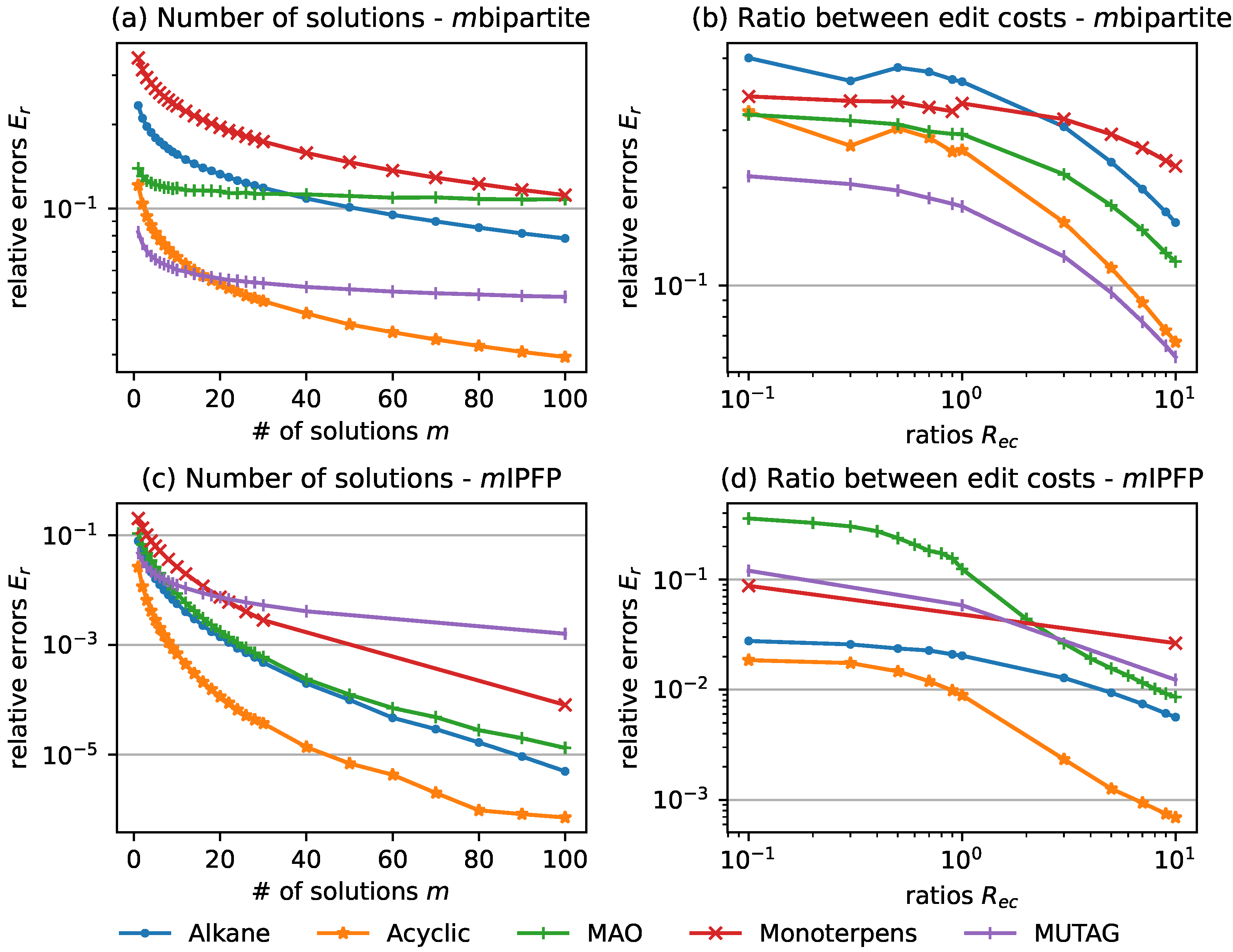
 Figure 2 shows the effect of the two factors, namely “# of solutions” and the ratio between vertex and edge edit costs $R_{ec}$, on the relative error $E_r$ defined in (5), considering the mbipartite and mIPFP heuristics on five datasets. The  Figure 2a,c on the left side exhibit how $E_r$ drops with the increase of the “# of solutions” m. In most cases, $E_r$ drops rapidly when the solution number increases from 1 to around a certain number $\mathbb{N}$, and reaches at a relatively small value; the tendency mitigates afterwards. $\mathbb{N}$ is around 20 for mbipartite and 10 for mIPFP. Take datasets Alkane and Acyclic for examples. When using mbipartite, $E_r$’s on these two datasets drop respectively from 0.23 to 0.08, and from 0.12 to 0.03, as m increases from 1 to 100; when using mIPFP, $E_r$’s drop respectively from 0.08 to $5\times {10}^{-6}$, and from 0.03 to $7.2\times {10}^{-7}$. This result indicates that an adequately large number of solutions is necessary, thus a trade-off decision between stability and time complexity needs to be made for different applications.

The  Figure 2b,d on the right side reveal the relation between $E_r$ and the ratio $R_{ec}$. The edge costs are set to 1 and the vertex costs to be the ratio value (for insertions, removals, and substitutions). The removal costs of vertices (resp. edges) are set to 0 if vertices (resp. edges) are not labeled. For both mbipartite and mIPFP, $E_r$ is relatively large when the ratio is smaller than 1, namely when edge costs are bigger than vertex costs, and drops with the increase of the ratio. We can observe that a larger ratio leads to higher stability. Take datasets Alkane and Acyclic for examples. When using mbipartite, $E_r$’s on these two datasets drop respectively from 0.5 to 0.16, and from 0.34 to 0.07, as $R_{ec}$ increases from 0.1 to 10; when using mIPFP, $E_r$’s drop respectively from 0.03 to $5.6\times {10}^{-3}$, and from 0.02 to $6.9\times {10}^{-4}$. A possible cause of this phenomenon is that large edge costs amplify the arbitrariness of the edge edit operations. For graphs with n vertices, there are $n^2$ possible edges that can be inserted, removed, and substituted, which causes more uncertainty when constructing edit paths and computing their costs. Taking IPFP for instance, large edge costs lead to a big cost matrix $\mathbf{Q}$ in (4), implying the possibility of more variance on the value of the term $g{\mathbf{x}}^{\top }\mathbf{Q}\mathbf{x}$. Many edit costs given by domain experts are in accordance with this empirical rule, such as the ones in [17]. In the next section, we further validate the relevance of stability and prediction performance benefitting from an edit cost learning method.

4.2. Stability vs. Prediction Performance

As stated in the Introduction, the choice of edit costs has a major impact on the computation of graph edit distance, and thus on the performance associated with a prediction task. To challenge these predefined expert costs with how they can improve the prediction performance, methods to tune the edit costs and thus the GED were proposed in the literature [23,32,33]. These methods provide an opportunity to observe the connection between the prediction performance of GEDs and the choices of edit costs, which further relate to the GED stability, as examined in Section 4.1.

To inspect this relevance, we utilize a state-of-the-art cost learning algorithm [23], where the edit costs are optimized according to a particular prediction task. An alternate iterative procedure is proposed to preserve the distances in both the graph space (GEDs) and target space (Euclidean or Manhattan distances between targets), where the update on edit costs obtained by solving a constrained linear problem and a re-computation of the optimal edit paths according to the newly computed costs are performed alternately. The GEDs with optimized edit costs are then used to train a k-nearest-neighbors (KNN) regression [34] model. KNN predicts the property value or class of an object based on the value or class of its neighbors. It has been widely used for various types of data, such as traffic [35], infrared vision [36], sensors [37], and graphs [38]. Thus, it is suitable for the current experiments. Experiments on Alkane and Acyclic show that optimized costs gain a significant improvement in accuracy compared to random or expert costs [1].

Table 1. Average and standard deviation of fitted edit costs’ values.

Dataset	Edit Cost	Distance	${\mathit{c}}_{\mathbf{ni}}$	${\mathit{c}}_{\mathbf{nr}}$	${\mathit{c}}_{\mathbf{ns}}$	${\mathit{c}}_{\mathbf{ei}}$	${\mathit{c}}_{\mathbf{er}}$	${\mathit{c}}_{\mathbf{es}}$
Alkane	bipartite	Euclidean	26.45 ± 0.48	26.24 ± 0.60	-	0.13 ± 0.06	0.14 ± 0.09	-
		Manhattan	26.67 ± 0.37	26.63 ± 0.58	-	0.11 ± 0.04	0.11 ± 0.06	-
	IPFP	Euclidean	26.12 ± 0.24	25.88 ± 0.25	-	0.74 ± 0.23	0.78 ± 0.23	-
		Manhattan	25.94 ± 0.38	25.71 ± 0.44	-	0.89 ± 0.30	0.77 ± 0.29	-
Acyclic	bipartite	Euclidean	13.81 ± 0.48	13.83 ± 0.80	10.46 ± 0.40	1.37 ± 0.46	1.45 ± 0.46	1.41 ± 0.09
		Manhattan	13.76 ± 0.39	14.14 ± 0.57	10.28 ± 0.44	1.44 ± 0.20	1.45 ± 0.19	1.45 ± 0.07
	IPFP	Euclidean	11.61 ± 0.45	11.68 ± 0.43	11.07 ± 0.53	4.49 ± 0.30	4.46 ± 0.24	4.48 ± 0.18
		Manhattan	11.52 ± 0.40	11.40 ± 0.40	10.61 ± 0.52	4.50 ± 0.31	4.50 ± 0.31	4.50 ± 0.10

summarizes the optimized values of edit costs.

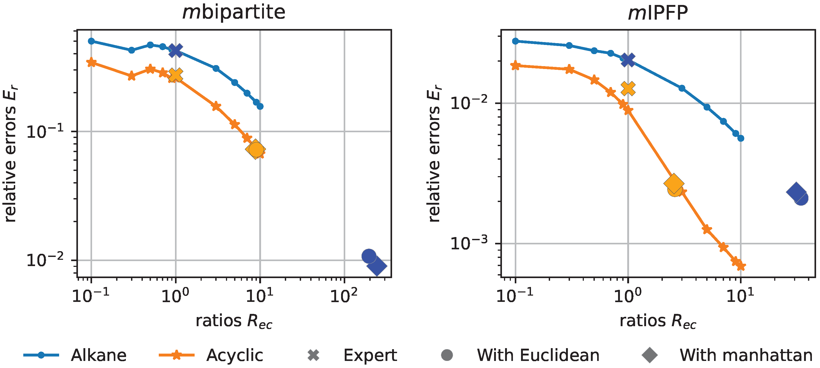
We then examine the stability of the two heuristics when using these edit costs.  Figure 3 demonstrates the relations between the relative errors $E_r$ and the ratios $R_{ec}$ between vertex and edge costs (See Section 3.2 and  Figure 2 for more details). Therein, the colors represent datasets (i.e., blue for Alkane and orange for Acyclic), and shapes represent different edit costs, with 🞮, ⬤, and ⯁ respectively for the expert costs, the optimized costs using the Euclidean and Manhattan distances. When applying mIPFP, for the expert costs, $R_{ec}$’s for the two datasets are both 1, and $E_r$’s are 0.02 for Alkane and 0.013 for Acyclic; when using the Euclidean distance, $R_{ec}=34.21$, $E_r=0.002$ for Alkane, and $R_{ec}=2.6$, $E_r=0.002$ for Acyclic; when using the Manhattan distance, $R_{ec}=3.11$, $E_r=2.33\times {10}^{-3}$ for Alkane, and $R_{ec}=2.55$, $E_r=2.68\times {10}^{-3}$ for Acyclic. It can be observed that the optimized costs correspond to much higher ratios and an order of magnitude lower relative errors than the expert costs. Similar conclusions can be observed for mbipartite as well. Thus, an empirical conclusion can be derived: the obtained optimized edit costs correspond to higher stability of GEDs, while obtaining a higher performance.

5. Conclusions and Future Work

In this paper, we conducted analyses of the GED heuristics’ stability, which is the first time it is formally investigated in the literature. After defining an (in)stability measure, namely, the relative error, we show the strong connection of the stability with the number of random initial candidates of multi-start GED heuristics and the relation between vertex and edge edit costs. Experiments on five datasets and two GED heuristics indicate that the proper choice of these factors can reduce the relative error by more than an order of magnitude. A further investigation indicates higher stability of GED computation corresponds to the optimized edit costs and thus better prediction performance, where an edit cost learning algorithm is applied to optimize the performance and the k-nearest neighbor regression for prediction.

There are still several challenges to address in future work. First, examining other influential factors and conducting theoretical analyses can help deepen understanding of the stability of the heuristics. Second, it will be helpful to perform more thorough experiments, including other state-of-the-art GED heuristics on datasets from a wider range of fields and statistical properties. Third, higher stability comes with the cost of higher time complexity. Methods that can better balance the stability, time complexity, and prediction performance in practice need to be developed.