Selection of Relevant Geometric Features Using Filter-Based Algorithms for Point Cloud Semantic Segmentation

Abstract

Semantic segmentation of mobile LiDAR point clouds is an essential task in many fields such as road network management, mapping, urban planning, and 3D High Definition (HD) city maps for autonomous vehicles. This study presents an approach to improve the evaluation metrics of deep-learning-based point cloud semantic segmentation using 3D geometric features and filter-based feature selection. Information gain (IG), Chi-square (Chi2), and ReliefF algorithms are used to select relevant features. RandLA-Net and Superpoint Grapgh (SPG), the current and effective deep learning networks, were preferred for applying semantic segmentation. RandLA-Net and SPG were fed by adding geometric features in addition to 3D coordinates (x, y, z) directly without any change in the structure of the point clouds. Experiments were carried out on three challenging mobile LiDAR datasets: Toronto3D, SZTAKI-CityMLS, and Paris. As a result of the study, it was demonstrated that the selection of relevant features improved accuracy in all datasets. For RandLA-Net, mean Intersection-over-Union (mIoU) was 70.1% with the features selected with Chi2 in the Toronto3D dataset, 84.1% mIoU was obtained with the features selected with the IG in the SZTAKI-CityMLS dataset, and 55.2% mIoU with the features selected with the IG and ReliefF in the Paris dataset. For SPG, 69.8% mIoU was obtained with Chi2 in the Toronto3D dataset, 77.5% mIoU was obtained with IG in SZTAKI-CityMLS, and 59.0% mIoU was obtained with IG and ReliefF in Paris.

1. Introduction

Three-dimensional (3D) point clouds are one of the most significant data sources, providing an accurate 3D representation of the world, and have been deployed in various applications, such as urban geometry mapping, autonomous driving, virtual reality, cultural heritage, augmented reality, and more [1,2,3,4]. Point clouds are a useful data type for representing and processing objects in the environment because they contain 3D information, such as geometry, color, intensity, normality, and more. Additionally, 3D point clouds provide more information about the geometric structure of objects than 2D images and allow sensor systems to perceive the environment better [5].

The development of automated artificial intelligence technologies has recently enabled the widespread usage of autonomous systems [6]. Robust and real-time sensing of the environment with high spatial accuracy is an important requirement for autonomous driving [7]. Additionally, precise positioning is a vital issue for autonomous driving. To fulfill these tasks, many sensors such as RGB camera for detection, light detection and ranging (LiDAR), depth camera or Radar sensors are added to autonomous vehicles. Because they provide direct space measurements, precise and quick 3D representations of the world, LiDARs have become a critical component in perception systems. LiDAR sensors are widely used to reconstruct the shape and surface of objects [8]. Mobile LiDAR point clouds are data obtained using laser scanners mounted on a moving vehicle. Mobile LiDAR point clouds provide useful data for many applications such as road network management, architecture and urban planning, and 3D high definition (HD) city maps for autonomous vehicles [9]. In particular, mobile LiDAR point clouds are expected to be the main data source used for autonomous driving and decision makers to produce detailed 3D High Definition (HD) maps. Successful execution of all these tasks is made possible by assigning each point in the point cloud to the correct semantic tag and performing the 3D scene analysis correctly [10]. Evaluating the singular features of the points together and collecting them under a meaningful cluster is called semantic segmentation [11].

Point cloud semantic segmentation has become an important research topic in the last decade. Traditionally, point cloud semantic segmentation relies on machine learning algorithms and rule-based methods that define a set of discriminatory rules to distinguish points for each class. However, these methods are insufficient for accurate semantic segmentation of complex, irregular, and large point cloud data generated in dynamic environments [12]. Deep learning methods, which had successful results in classification, detection, and segmentation in 2D images [13,14,15,16,17], have also been used in point cloud semantic segmentation. Initially, projection and voxelization methods were developed to regularize the point cloud with preprocessing steps for point cloud semantic segmentation based on 2D images. Voxelization requires a significant computational cost for large-scale dense 3D data because memory and compute requirements rise cubically, when the data are scaled up. In projection-based methods, 3D information loss may occur while the point cloud is projected to a two-dimensional plane. Point-based deep learning models have been developed in recent years to overcome these difficulties [9]. Although point cloud structure makes it potentially challenging for the DL approach to process the point cloud directly, point-based methods have advantages, as they prevent information loss and have no preprocessing step.

This study aims to examine the effects of 3D geometric features and appropriate feature selection in the accuracy of deep-learning-based point cloud semantic segmentation. RandLA-Net [18] and SPG [19] methods, which are up-to-date approaches, are used for semantic segmentation. Each point in the point cloud is defined by a 3D feature vector. Thus, helpful features are provided to the deep learning network. Furthermore, the most effective features were determined by filter-based feature selection algorithms, and the semantic segmentation results were improved. A study is presented to investigate the comparative performances of filter-based information gain (IG), Chi-squared (Chi2) [20], and ReliefF [21] for point cloud semantic segmentation. Experiments were carried out on mobile LiDAR point clouds, which are an important data source for autonomous driving. Large-scale outdoor benchmark MLS datasets Toronto3D [22], SZTAKI-CityMLS [23], and Paris-CARLA-3D [24] were chosen as the datasets.

2. Related Works

Deep learning approaches are used for point cloud semantic segmentation because of the inability of machine learning approaches to provide sufficient performance from large and complex data. The approaches in the first deep learning studies are usually based on 2D projection [25] and voxelization [26]. After projection-based and voxelization approaches, DL approaches fed directly with point cloud have been developed. Therefore, it is possible to collect semantic segmentation approaches under three main headings: point-based, voxel-based, and projection-based.

2.1. Point Cloud Semantic Segmentation with Point-Based Methods

The first point-based methods are point-wise multi-layer perceptrons (MLPs). Point-wise MLPs learn the properties of each point through shared MLPs. However, the relationship between the points is ignored, since the points are evaluated individually. PointNet [27] was developed for the first time as a unique method that directly uses the point cloud. PointNet++ [28] is provided as an enhanced version of PointNet. PointNet++ uses a hierarchical neural network that employs PointNet recursively on the input point set. PointSIFT [29] is a PointNet-like algorithm developed based on the Scale Invariance Feature Transform (SIFT) algorithm [30] used in 2D images. Engelmann et al. [31] proposed a combination of K-clustering and KNN to define two neighborhoods in world space and feature space separately. PointWeb [32] defines the relationship between points using the Adaptive Feature Adjustment (APA) module. RandLA-Net [18] proposed a local feature aggregation module used to capture complex local features and spatial relationships. ShellNet [33] is a permutation-invariant convolution that works directly on the point cloud.

To develop fixed MLPs of point-wise approaches, point convolution methods attempt to recognize weights based on learned features with convolutions with more inputs. Thomas et al. [34] present Kernel Point Convolution (KPConv) that is inspired by image-based convolution, but it uses kernel points to define the area where the kernel weight is applied instead of the kernel pixel used by image-based convolution. PointCNN [35] that applies $\kappa$ transformation to the input points prevents the loss of shape information and variance in the point order resulting from applying direct convolution. SpiderCNN [36] calculates the distance order of neighboring points and generates a family of polynomial functions with different weights for each neighbor. ConvPoint [37] includes a continuous convolution operation that learns the weighted sum from the feature convolution operation and simple MLP operations of spatial features.

Graph-based methods construct point clouds as super graphs and feed a graph convolution network by extracting local shape information from neighbors. The graph-based methods assume points as nodes of a graph, and point relationships are defined as edges [38]. DGCNN [39] obtains local features using the nearest points. Then, EdgeConv operators, which are edge convolutions, are used to extract global shape features using local features. 3D-GCN [40] proposes deformable kernels for shift and scale-invariant features. The SPG method [19], similar to DGCNN, considers the point cloud as a super point graph, and establishes point relations as edges. PointNet is used for embedding before the final prediction. DPAM [41] offers a deep learning architecture designed to dynamically sample and group points.

2.2. Point Cloud Semantic Segmentation with Voxel-Based Methods

Voxel-based approaches do not process points individually, but by grouping them into regular geometric shapes. Point clouds are transformed into structured data. These transformations cause a loss of information and resolution in point clouds. The first developed algorithms performed semantic segmentation by applying 3D convolutions to the generated voxels [23]. VoxNet [42], one of the most popular methods, defines the point cloud as an occupancy grid as input to CNNs. CNN models are widely preferred for voxel-based semantic segmentation. In addition, there are methods that apply semantic segmentation with hand-crafted features calculated within voxels [43]. The disadvantage of voxel-based approaches is the unnecessary memory usage caused by empty voxels. To overcome this problem, some approaches are proposed in the literature [44].

2.3. Point Cloud Semantic Segmentation with Projection-Based Methods

Projection-based methods project the point cloud to a two-dimensional plane. Similar to voxel-based approaches, the point cloud is transformed from an irregular structure to a regular one. Inspired by the SqueezeNet [45] architecture, SqueezeSeg [46] generates a range image by applying spherical projection to the point cloud for semantic point cloud segmentation. SqueezeSegv2 [7] has been presented in the literature with some improvements on SqueezeSeg. Another approach that has emerged recently is the RangeNet architecture [47], which was inspired by the Darknet53 architecture. SalsaNext [48], the enhanced version of SalsaNet [49], which adds a dilated convolution stack with 1 × 1 and 3 × 3 cores to the head of the network to improve context information. Additionally, there are studies that apply classical image segmentation algorithms after reducing the point cloud to the image plane [50,51]. Multi-view PointNet [52] purposes aggregation of 2D multi-view image features into 3D point clouds. There are also algorithms that perform object detection and labeling with the bird’s-eye-view method [53].

3. Materials and Methods

3.1. Datasets

3.1.1. Toronto-3D

Toronto-3D dataset [22] is a large-scale urban outdoor mobile LiDAR dataset for semantic segmentation. The point cloud was captured by a vehicle-mounted Teledyne Optech Maverick MLS system. The dataset has approximately 78.3 million points in 1 km of the road segment. The point cloud density is approximately 1000 points/m${}^2$. Each point is defined with 10 attributes; 3D coordinates of the point (x, y, z), color (red, green, blue), intensity, GPS time, scan angle rank and label. Object classes were defined as road, road marking, natural, building, utility line, pole, car, fence, and unclassified. The dataset is divided into four parts (L001, L002, L003, and L004), each covering a distance of 250 m. L001, L003, and L004 are used for the training set, and L002 is used for the testing set, following the guidelines from the original paper on the Toronto-3D dataset.

3.1.2. SZTAKI-CityMLS

The SZTAKI-CityMLS Point Cloud dataset (SZTAKI-CityMLS) [23] has been used to evaluate 3D semantic point cloud segmentation algorithms in urban environments based on mobile laser scanning (MLS) measurements of a Riegl VMX-450 mobile mapping system. SZTAKI-CityMLS dataset contains around 327 Million annotated points from various urban scenes, including main roads with both heavy and solid traffic, public squares, parks, sidewalk regions, various types of cars, trams and buses, several pedestrians, and diverse vegetation. Since there is no official division in the SZTAKI-CityMLS dataset, four parts of the dataset consisting of six parts were used for training, one part for validation, and one part for testing.

3.1.3. Paris-CARLA-3D

The Paris-CARLA-3D (PC3D) [24] dataset was created with a mobile mapping system including a LiDAR (Velodyne HDL32) inclined at 45° to the horizon and a 360° poly-dioptric Ladybug5. Paris-Carla-3D consists of two datasets: real (Paris) and synthetic (Carla). The dataset consists of data collected on a route 550 m in Paris and 5.8 km in CARLA. Only the real part, Paris, was used in this study. The Paris dataset consists of six point clouds containing 10 million points (S0 to S5), with a total of 60 million points. The points are labeled under 23 classes. In addition, since the mobile LiDAR system also includes a camera, the point cloud is colored (RGB) due to the necessary orientation processes. Although the real part does not cover a large area (it includes three streets in the center of Paris), it is captured in areas where the number and variety of urban objects, pedestrian movements and vehicles are dense, allowing for various analyses.

3.2. Filter-Based Feature Selection

Although more features are used to address the lack of information and increase the distinctiveness of algorithms, not all of these features have the same effect. Some features may be more suitable for semantic segmentation, while others may be irrelevant. Feature selection is defined as the task of determining the minimum number of features that will accurately represent the data [54]. Feature selection algorithms are used to find compact and robust subsets of relevant and informative features to enhance accuracy, improve computational efficiency with respect to both time and memory consumption, and retain relevant features. Feature selection methods can be grouped as filter-based, wrapper-based, and embedded methods. Since both wrapper-based and embedded methods contain classifier algorithms, they can have better selection performance than filter-based methods. However, this performance is still dependent on the applied classifier, and the optimum properties may change when the classifier changes. Filter-based methods are independent of the classifier. Feature selection methods are simple and efficient, as they calculate the feature importance score based on only training data [10].

3.2.1. Information Gain

Information Gain (IG), an entropy-based feature selection algorithm widely used in machine learning, can be defined as the amount of information provided by features. With the inflammation gain, the importance of the features for classification is measured, and it is decided which features are appropriate to use [55]. It is widely used in the literature, especially for text classification.

$$G(D,t)=-\sum _{i=1}^{m}P\left(C_i\right)logP\left(C_i\right)+P\left(t\right)\sum _i^{m}P\left(C_i\right|t)logP\left(C_i\right|t)+P\left(\overline{t}\right)\sum _i^{m}P\left(C_i\right|\overline{t})logP\left(C_i\right|\overline{t})$$

(1)

where C is set of feature, $C_i|t$ is feature set without feature t. The $G(D,t)$ value shows the importance of the feature. The t features with the highest $G(D,t)$ should be selected. m is the number of class.

3.2.2. Chi2 Algorithm

The Chi2 feature selection algorithm [20], which is a filter-based feature selection technique, is based on the Chi-squared (${\chi }^2$) statistic. The basic working principle of this method is to calculate how much the (${\chi }^2$) statistic differs from the actual value and the expected value. The Chi2 algorithm calculates the correlation between two variables and the degree of independence from each other. When Chi2 is used for feature selection, it predicts the independence of the observation class with a particular feature in the dataset [56]. The null hypothesis establishes that two variables are unrelated or independent. The ${\chi }^2$ value is calculated for every feature value i and class j using Equation (2).

$${\chi }^2=\sum _{i=1}^r\sum _{j=1}^k\frac{{(A_{ij}-E_{ij})}^2}{E_{ij}}$$

(2)

where r defines the number of distinct values in a feature vector. k is the number of classes. The number of samples with a value of i in class j is represented as $A_{ij}$, and the expected number of samples with a value of i in class j is represented as $E_{ij}$.

3.2.3. ReliefF

The ReliefF algorithm [21] was developed based on the Relief method used by [57] for solving two-class features. ReliefF algorithm is a feature selection algorithm that assigns higher weights to features related to classes, quickly eliminates irrelevant features, and provides high efficiency in solving multiple classification problems. ReliefF aims to measure the quality of the features based on the distinction it makes between randomly selected samples which were close to each other. These were selected from the training set [56]. The k nearest neighbors with the same label and k neighbors with different classes are selected for the selected random points. If samples with the same label have different values for a certain feature, the weight of the feature is decreased. If samples with different labels have different values for a certain feature, the weight of the feature is increased. The $R_f$ score is computed using Equation (3).

$$R_f\left(x_i\right)=\frac{1}{N}\sum _{t=1}^N\left\{-\frac{1}{k}\sum _{x_i\in NH\left(y\right)}^{}diff(x_{t,i},x_{j,i})+\sum \frac{1}{k}\frac{P\left(y\right)}{1-P\left(y_i\right)}\sum _{x_j\in NM(x_i,y)}^{}diff(x_{t,i},x_{j,i})\right\}$$

(3)

where $R_f\left(x_i\right)$ is the score of $x_i$. $y_i$ is the class label of the sample $x_t$. $P\left(y\right)$ defines the probability of a sample being from class y. $x_{t,i}$ presents the values of $x_t$ on feature $x_i$ and $diff(·)$ is the function used to calculate the difference between $x_{t,i}$ and $x_{j,i}$. $NH(x_i,y)$ represents neighbors having the same class label. $NM(x_i,y)$ represents neighbors that have different class labels [54]. N is the number of samples in input data.

3.3. 3D Geometric Features

Eigen-based features describe the local geometry around the point and are commonly used in LiDAR processing. Neighboring points around a point can be determined using a sphere or other geometric shape, with that point as the center. This neighborhood area is called the support area [58]. In this study, the support area was determined with a sphere. The critical parameter when creating the support area is the radius of the sphere. The sphere radius that best describes the local geometry should be determined.

Eigen-based features are calculated by the eigenvalues (${\lambda }_1$, ${\lambda }_2$, ${\lambda }_3$) of the eigenvectors ($v_1$, $v_2$, $v_3$) derived from the covariance matrix of any point p of the point cloud [10]:

$$cov\left(N\right)=\frac{1}{N}\sum _{p\in N}(p-\overline{p}){(p-\overline{p})}^T$$

(4)

where $\overline{p}$ is the centroid of the neighborhood N. The calculated eigen-based features using eigenvalues: linearity (5), planarity (6), sphericity (7), omnivariance (8), anisotropy (9), eigenentropy (10), surface variation (11), and verticality (12). In addition to eigen-based features height differences (13) in the support area of a point have been added.

$$Linearity=({\lambda }_1-{\lambda }_2)/{\lambda }_1$$

(5)

$$Planarity=({\lambda }_2-{\lambda }_3)/{\lambda }_1$$

(6)

$$Sphericity={\lambda }_3/{\lambda }_1$$

(7)

$$Omnivariance=\sqrt[3]{{\lambda }_1{\lambda }_2{\lambda }_3}$$

(8)

$$Anisotropy=({\lambda }_1-{\lambda }_3)/{\lambda }_1$$

(9)

$$Eigenentropy=\sum _{i=1}^3{\lambda }_{i}ln{\lambda }_i$$

(10)

$$Surfacevariation={\lambda }_3/({\lambda }_1+{\lambda }_2+{\lambda }_3)$$

(11)

$$Verticality=1-{\lambda }_3/({\lambda }_1+{\lambda }_2+{\lambda }_3)$$

(12)

$$Heightdifference=Z_{max}-Z_{min}$$

(13)

3.4. RandLA-Net

Random sampling and an effective local feature aggregator (RANDLA-Net) [18] was used as the segmentation algorithm. A large-scale point cloud with millions of points inevitably requires these points to be down-sampled efficiently without losing their beneficial point properties in order to process it with a deep neural network. In RandLA-Net, a simple and fast random sampling approach has been used to drastically reduce point density while applying a carefully designed local feature aggregator to preserve remarkable features. The computational complexity is independent of the total number of entry points, i.e., it is fixed time and thus inherently scalable. The local feature aggregator module is designed to effectively preserve complex local structures by explicitly considering neighboring geometries and significantly increasing receptive fields. This module consists of feed-forward MLPs, so it is computationally efficient.

A local feature aggregation module is applied to each 3D point in parallel, and it consists of three neural units: (1) local spatial encoding (LocSE), (2) attentive pooling, and (3) a dilated residual block. Given a point cloud where each point has certain features (RGB and 3D geometric features for this study), the local spatial coding unit determines the properties of each point within the neighborhood area of that point. Thus, the LocSE unit clearly observes the local geometric patterns, and it can learn the complex local structures of the whole network effectively. The K-nearest neighbors (KNN) algorithm based on the Euclidean distance is used to determine the neighborhood area. For each of the nearest K points $\left\{p_i^1\dots p_i^k\dots p_i^K\right\}$ of the center point $p_i$, the relative point position is encoded as follows:

$$r_i^k=MLP(p_i\oplus p_i^k\oplus (p_i-p_i^k)\oplus \parallel p_i-p_i^k\parallel )$$

(14)

where $p_i$ and $p_i^k$ are the 3D coordinates of points. $\parallel •\parallel$ calculates the Euclidean distance. Neighboring point $p_i^k$, the encoded relative point positions $p_i^k$ and point features $f_i^k$ are combined to create augmented feature vector ${\widehat{f}}_i^k$. The LocSE unit produces a new set of local features ${\widehat{\mathbf{F}}}_i=\left\{{\widehat{\mathbf{f}}}_i^1\dots {\widehat{\mathbf{f}}}_i^k\dots {\widehat{\mathbf{f}}}_i^K\right\}$.

In the attentive pooling unit, a unique attention score is calculated using a shared function $g\left(\right)$ for each local feature ${\widehat{\mathbf{F}}}_i=\left\{{\widehat{\mathbf{f}}}_i^1\dots {\widehat{\mathbf{f}}}_i^k\dots {\widehat{\mathbf{f}}}_i^K\right\}$.

$$s_i^k=g({\widehat{\mathbf{f}}}_i^k,\mathbf{W})$$

(15)

where $\mathbf{W}$ is the learnable weights of a shared MLP. Features are weighted summed by using attention scores, and informative feature vector ${\tilde{\mathbf{f}}}_i$ is produced.

$${\tilde{\mathbf{f}}}_i=\sum _{k=1}^K({\widehat{\mathbf{f}}}_i^k\times {\mathbf{s}}_i^k)$$

(16)

Two sets of LocSE and attention pooling are stacked to increase the receptive field size within a dilated residual block. After the first LocSE/Attention Pooling process, information was obtained from K neighbor points and then again from $K^2$ points by observing the K neighbors of the receptive field in the first process. Thus, the efficiency of the algorithm has been increased by expanding the receptive field [18].

3.5. Superpoint Graph (SPG)

The Superpoint Graph (SPG) [19] is a deep-learning-based approach developed for the semantic segmentation of large-scale point clouds based on partition into simple shapes. The point cloud is defined by superpoint graphs derived from geometrically homogeneous elements. The advantages of SPG are that it can classify a part of the object rather than a point or voxel, it can provide long-range modeling by defining the SPG size according to the object parts in the scene, and it can describe the relationship between adjacent objects in detail. A deep learning architecture consisting of PointNets and graph convolutions is implemented in detail without significant loss of information.

SPG consists of three main steps. In the first step, the point cloud is divided into small and meaningful superpoints. The geometrically homogeneous partition is defined as the constant connected components of the solution of the generalized minimal partition problem. Secondly, point clouds are downsampled to a smaller number of points. The SPG can be computed from this partition. The SPG is a representation of the point cloud, defined as a directed graph ($G=S,E,F$) consisting of the set of superpoints S, superedges E, and features F characterizing the adjacency relationship between superpoints. $G_{vor}=(C,E_{vor})$ is defined as symmetric Voronoi adjacency graph of the input point cloud C. If one edge of the $E_{vor}$ considers a connection between S and T, Superpoints S and T are adjacent.

$$\epsilon =\{(S,T)\in S^2|\exists (i,j)\in E_{vor}\cap (S\times T)\}$$

(17)

Secondly, large point clouds are subsampled to a smaller number of point clouds, thus implementing PointNet. Finally, contextual segmentation is performed. SPG is smaller than graphs from the entire point cloud. Deep learning algorithms based on graph convolutions classify SPG’s nodes using edge features that increase long-range interaction.

3.6. Experimental Details

As a preprocessing step, local geometric properties were calculated for each dataset. The neighborhood area was determined for each point in order to calculate the local geometric properties. The neighborhood area was determined by the nearest point approach. In addition, a distance threshold has been applied to prevent the detection of unrelated neighbors to the point. The optimum parameters determined experimentally are 100 nearest neighbor points and 0.5 m distance threshold. Then, feature selection algorithms were applied to the geometric features. Thus, the aim was to determine the most suitable features for training and testing. The importance of the features were determined with Information Gain, Chi2 and ReliefF algorithms, respectively. Subsets were created with the selected features. Feature selection algorithms were implemented by using Scikit-learn library in Python [59] and WEKA workbench [60].

The Toronto3D and Paris datasets contain 3D coordinates (x, y, z) and RGB information. In the SZTAKI-CityMLS dataset, there are only 3D coordinates. In Toronto3D and Paris, the RGB values of the points are also used as features in the training. All of the deep learning experiments were implemented in a Python programming language and performed with a single GPU. RandLA-Net is applied by using Open3D-ML library [61]. As RandLA-Net training parameters, 200 epochs and 50 iterations in each epoch, learning rate 0.001, and batch size 2 were determined. We used 500 epoch and 1 iteration, learning rate 0.01, and a batch size of 2 for SPG. For the experiments, i7-11800H, 2.30 GHz processor, GTX 3070 graphics card, and 32 GB RAM hardware was used. The workflow of the study is shown in Figure 1. The results are evaluated by the mean Intersection over-Union (mIoU) and mean accuracy (MA).

$$\mathrm{mIoU}=\frac{1}{N}\sum _{c=1}^N\frac{P_c\cap G_c}{P_c\cup G_c}$$

(18)

$$\mathrm{MA}=\frac{1}{N}\sum _{c=1}^N\frac{P_{cc}}{G_c}$$

(19)

where $P_c$ and $G_c$, respectively, refer to predicted and ground-truth points that belong to class c. c∈ (1, 2, …, N) is the index of the class. $P_{cc}$ refers to number of true predictions for each class.

4. Results

4.1. Feature Selection and Creating Subsets

The most suitable feature subsets were determined through filter-based feature selection algorithms. In addition, training using all features and only 3D coordinates was conducted to emphasize the effect of feature selection. Feature importance values are calculated and ordered from largest to smallest. Specific breakpoints were determined as the threshold value, and features with importance less than that threshold value were eliminated. A different number of features were selected for each algorithm. In the Toronto3D dataset, four features with the highest importance value were selected with IG. We also selected three features with Chi2 and three features with ReliefF (Figure 2). While the height difference has the highest importance value in all three methods, the linearity is out of the dataset. In the SZTAKI-CityMLS dataset, seven features were selected with IG, three features with Chi2, and five features with ReliefF (Figure 3). In the Paris dataset, the same five features had highest importance, which was calculated with IG and ReliefF. Three features were selected with Chi2 (Figure 4).

After feature selection, subsets were created for training and testing. In order to examine the effect of geometric features, training and testing were carried out with different datasets. Since the Toronto 3D and Paris also contain RGB information, more feature combinations were created than the SZTAKI-CityMLS dataset. The ten subsets obtained from Toronto3D are named $T_1$ to $T_{10}$. Five subsets from $S_1$ to $S_5$ were produced from the SZTAKI-CityMLS data set. Ten subsets $P_1$ to $P_{10}$ were obtained from Paris. The descriptions of the subsets are given below.

For Toronto3D dataset:

• $T_1$: only 3D coordinates (x, y, z).
• $T_2$: 3D coordinates and RGB.
• $T_3$: 3D coordinates and all geometric features.
• $T_4$: 3D coordinates and 4 selected features with IG.
• $T_5$: 3D coordinates and 3 selected features with Chi2.
• $T_6$: 3D coordinates and 4 selected features with ReliefF.
• $T_7$: 3D coordinates, RGB and all geometric features.
• $T_8$: 3D coordinates, RGB, and 4 selected features with IG.
• $T_9$: 3D coordinates, RGB, and 3 selected features with Chi2.
• $T_{10}$: 3D coordinates, RGB, and 4 selected features with ReliefF.

For SZTAKI-CityMLS dataset:

• $S_1$: only 3D coordinates (x, y, z).
• $S_2$: 3D coordinates and all geometric features.
• $S_3$: 3D coordinates and 7 selected features with IG.
• $S_4$: 3D coordinates and 3 selected features with Chi2.
• $S_5$: 3D coordinates and 5 selected features with ReliefF.

For Paris dataset:

• $P_1$: only 3D coordinates (x, y, z).
• $P_2$: 3D coordinates and RGB.
• $P_3$: 3D coordinates and all geometric features.
• $P_4$: 3D coordinates and 5 selected features with IG.
• $P_5$: 3D coordinates and 3 selected features with Chi2.
• $P_6$: 3D coordinates and 5 selected features with ReliefF.
• $P_7$: 3D coordinates, RGB and all geometric features.
• $P_8$: 3D coordinates, RGB, and 5 selected features with IG.
• $P_9$: 3D coordinates, RGB, and 3 selected features with Chi2.
• $P_{10}$: 3D coordinates, RGB, and 5 selected features with ReliefF.

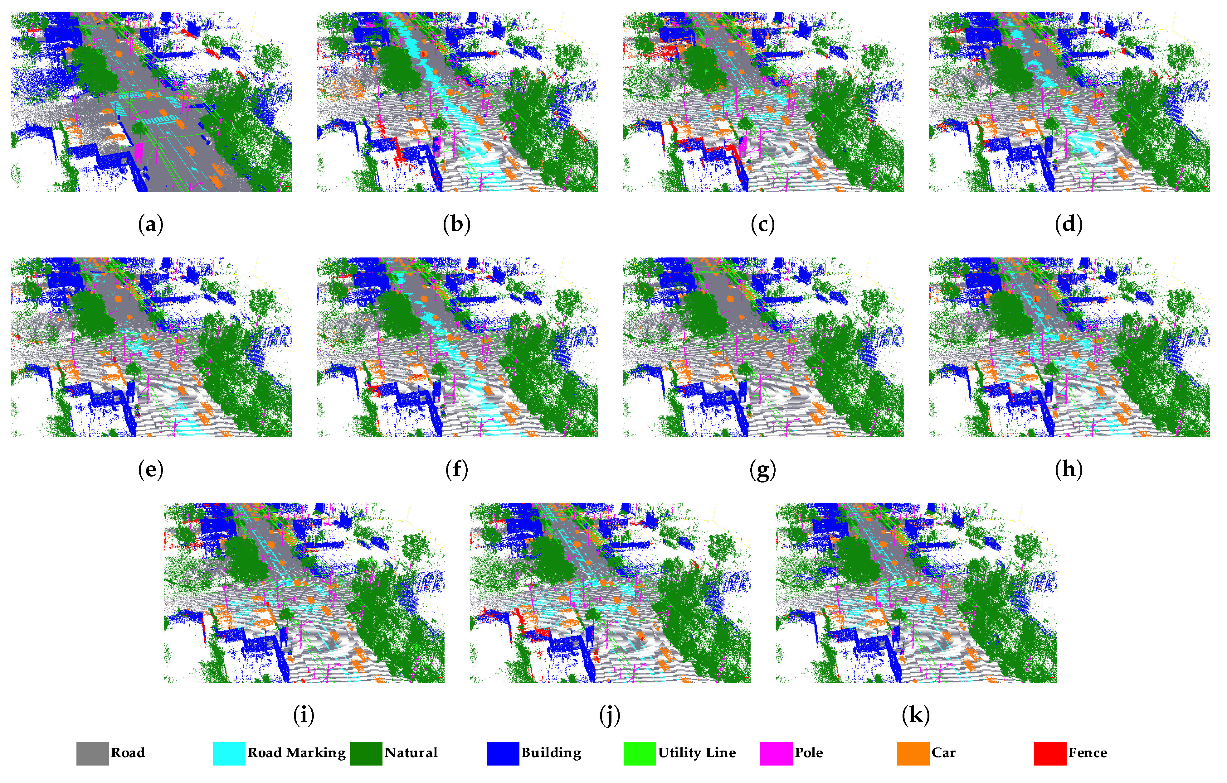
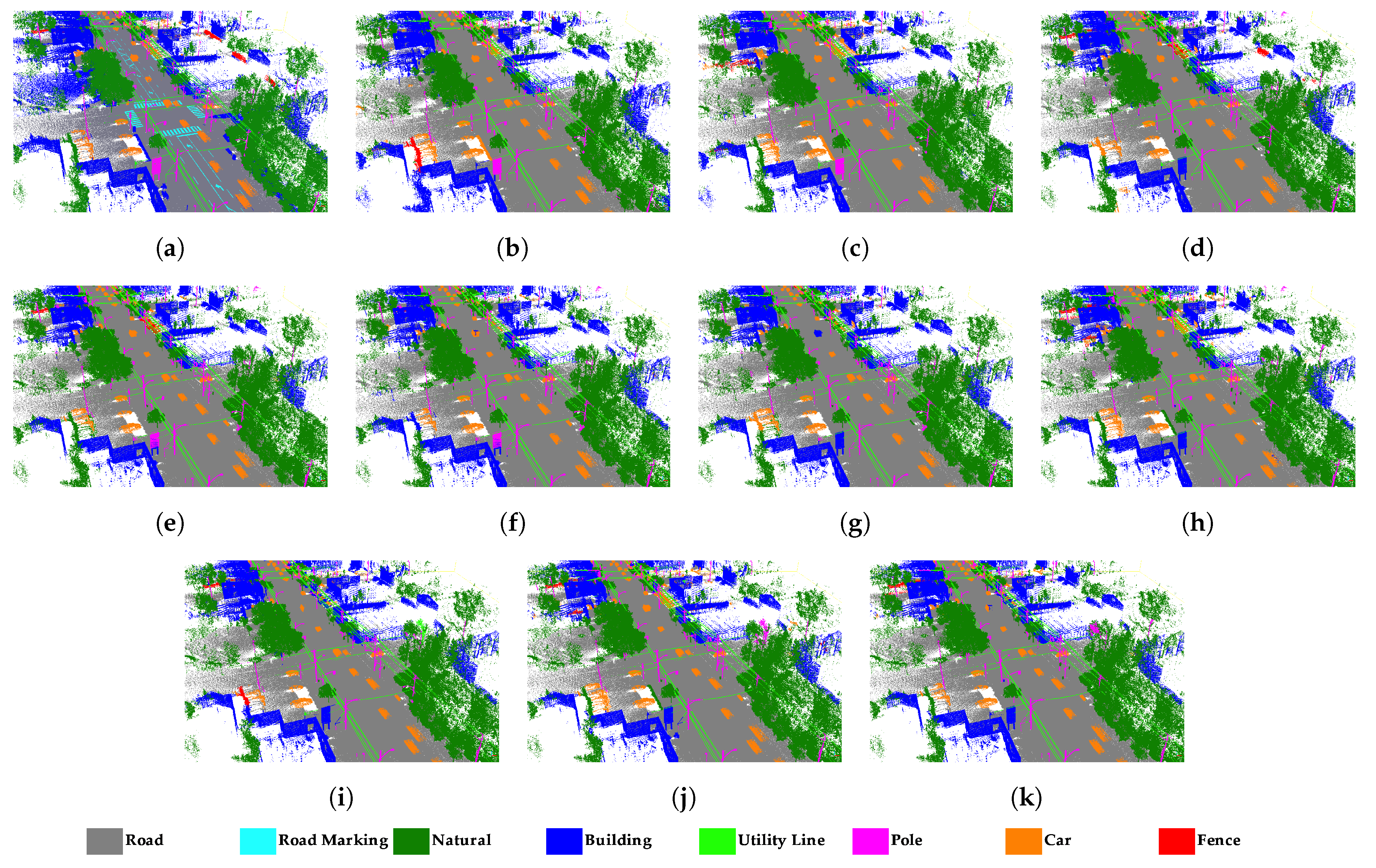
4.2. Results of Semantic Segmentation on Toronto3D

RandLA-Net and SPG algorithms were trained separately using each subset. The aim was to determine the most suitable feature subset for point cloud semantic segmentation. The process was repeated in the same way for each case.

For RandLA-Net, although the IoU value of the road marking class, where only 3D coordinates and geometric features are used, remained below 10%, when RGB information was included, close to 50% IoU was obtained. The highest IoU values were achieved in the natural class. It has over 90% IoU value in all subsets. Buildings are also classified with an IoU value of 92.2%. The highest IoU value in the Fence class was obtained with the $T_5$ subset as 31.9%. The highest value in mean accuracy was obtained as 87.4% using the $T_9$ subset. The second best result was obtained by using $T_8$ and $T_{10}$, where the mean accuracies are 87.2% for both subsets. The lowest mIoU and MA have the experiment with the $T_1$ subset containing only 3D coordinates. The mIoU and MA metrics for $T_1$ are 60.8% and 74.2%, respectively. The features selected with Chi2 have a greater increase in accuracy. Although this advantage was slight when used with RGB, the mean accuracy was 2.6% higher than $T_4$ and 4.2% higher than $T_6$ when using the $T_5$ subset. Class-based results are presented in the

Table 1. Class-based results of RandLA-Net on subsets of Toronto3D. Highest values are marked in bold.

Subset	Road	Road Mrk.	Natural	Building	Util. Line	Pole	Car	Fence	mIoU	MA
$T_1$	69.4	7.7	92.3	85.7	76.3	70.0	76.9	7.95	60.8	74.2
$T_2$	94.0	49.6	93.3	84.4	78.5	69.9	79.5	14.1	70.4	86.0
$T_3$	77.1	6.1	94.7	91.2	85.9	72.6	50.6	23.4	62.7	79.8
$T_4$	91.0	7.2	95.8	92.1	84.9	78.3	83.7	23.2	69.5	76.6
$T_5$	79.4	6.7	95.2	92.2	84.6	73.9	80.4	31.9	68.0	79.2
$T_6$	90.5	8.2	94.8	91.6	85.1	74.9	69.2	20.1	66.8	75.0
$T_7$	77.8	17.5	95.3	90.4	85.6	76.9	51.6	25.7	65.1	83.1
$T_8$	87.5	37.8	95.5	89.6	82.1	79.3	49.5	23.4	68.2	87.2
$T_9$	87.2	29.2	95.2	90.7	83.1	76.1	79.1	20.5	70.1	87.4
$T_{10}$	87.6	31.9	95.2	88.5	83.7	78.0	71.9	20.7	69.5	87.2

. The qualitative assessment is illustrated in Figure 5.

The road class has over 94% IoU on all subsets when using SPG. The entire road marking class could not be determined. Similar to RandLA-Net, SPG also does not have successful results from the fence class. The highest IoU value for the Fence class was reached in the $T_9$ subset. The SPG method was successful in building, natural, and car classes. Chi2 is superior to other methods in semantic segmentation of Toronto3D with SPG. The highest values in both mean accuracy and mIoU are achieved using three features selected with Chi2. In the $T_9$ subset, 75.9% MA and 69.8% mIoU was obtained. Subset $T_8$ has the second highest mIoU at 67.5%. $T_1$ has the lowest MA and mIoU values of 68.8% and 63.4%, respectively. The subsets $T_6$ and $T_{1}0$ containing the geometric features selected by the ReliefF method have lower accuracy than the other subsets. $P_8$ and $P_{10}$ containing selected features from IG and ReliefF have 5.7% higher mIoU than $P_7$. Subset $P_9$, which includes features selected with Chi2, also has 3.1% higher mIoU than $P_7$. Although adding the RGB value improves accuracy metrics, adding geometric features further increases accuracy. Class-based results are presented in the

Table 2. Class-based results of SPG on subsets of Toronto3D. Highest values are marked in bold.

Subset	Road	Road Mrk.	Natural	Building	Util. Line	Pole	Car	Fence	mIoU	MA
$T_1$	94.1	0.0	90.4	84.6	81.9	72.0	82.7	1.4	63.4	68.8
$T_2$	94.2	0.0	94.2	87.4	83.2	77.7	83.9	2.4	65.4	69.3
$T_3$	94.5	0.0	94.6	90.0	79.2	72.4	85.4	11.9	66.0	71.7
$T_4$	94.5	0.0	94.6	88.6	79.2	75.2	84.5	11.4	66.0	73.4
$T_5$	94.3	0.0	94.3	91.4	78.0	74.9	86.9	17.8	67.2	72.5
$T_6$	94.5	0.0	93.3	88.1	79.3	74.7	77.1	6.8	64.2	69.3
$T_7$	94.4	0.0	95.6	90.6	80.8	70.0	89.1	15.4	67.0	72.3
$T_8$	94.1	0.0	94.3	91.7	79.4	68.7	89.5	22.5	67.5	73.8
$T_9$	94.4	0.0	95.6	90.5	79.7	69.7	91.2	37.3	69.8	75.9
$T_{10}$	94.1	0.0	94.3	89.1	81.8	71.4	89.5	4.7	65.6	70.0

. The qualitative assessment is illustrated in Figure 6.

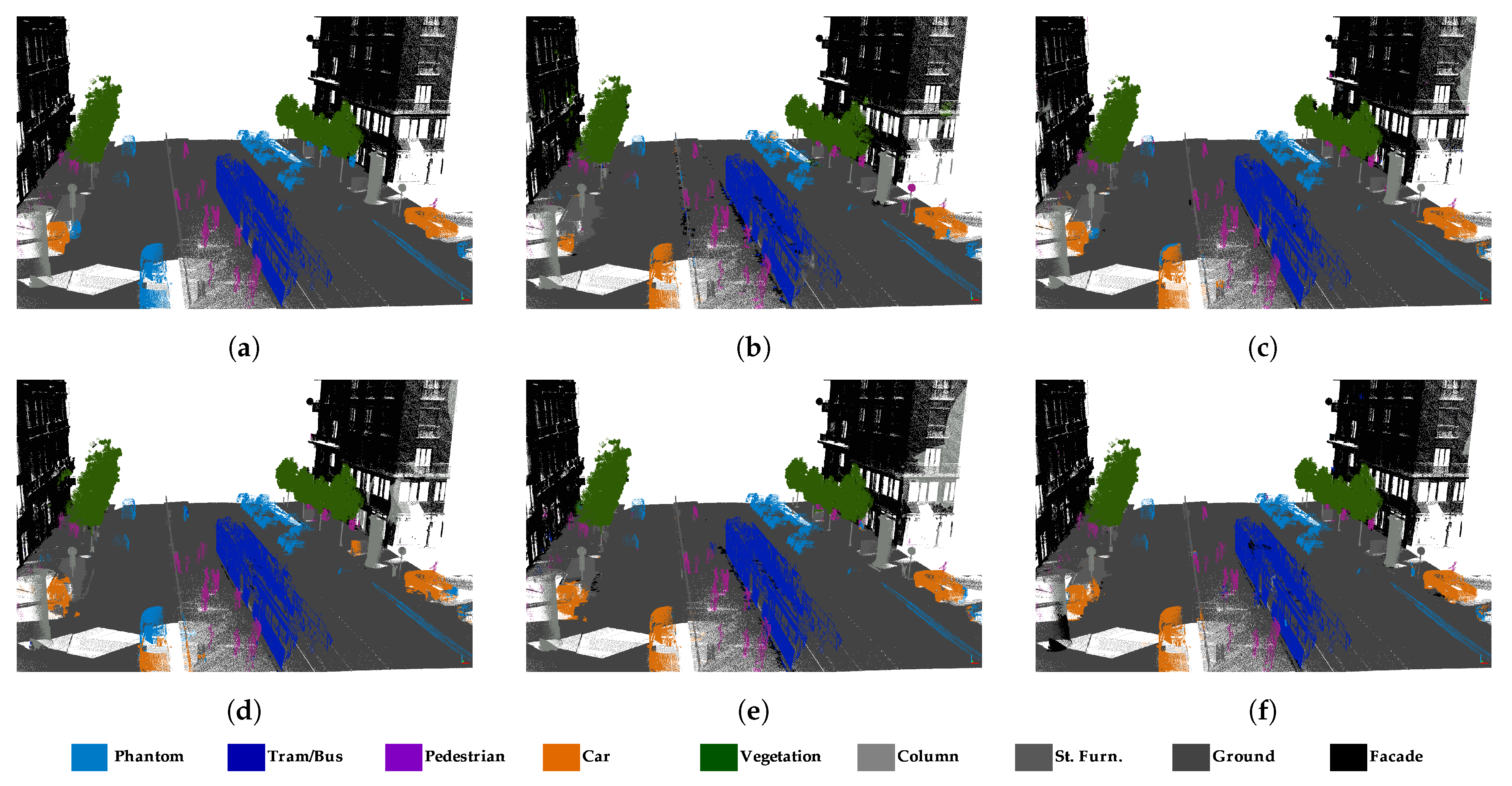
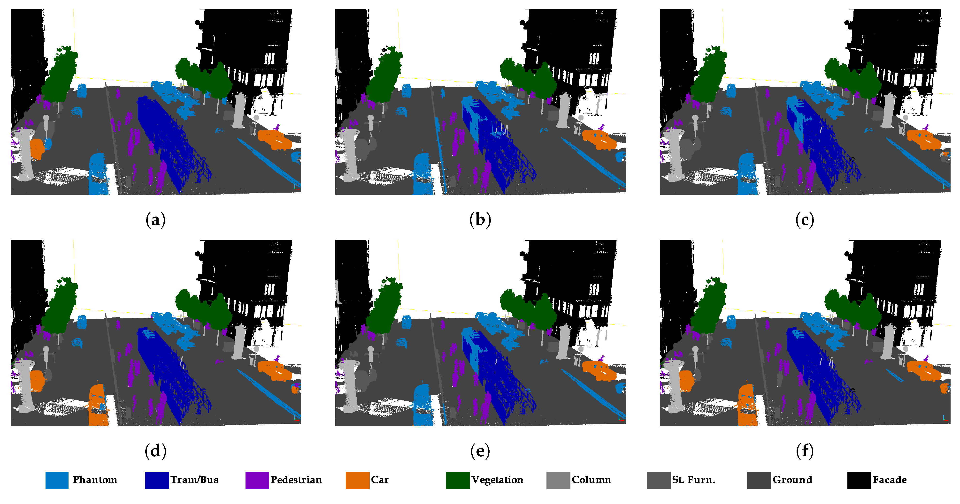
4.3. Results of Semantic Segmentation on SZTAKI-CityMLS

In the SZTAKI-CityMLS dataset, the IoU values of vegetation, ground, and facade classes are over 97% in all generated subsets with RandLA-Net. Although there were similar results in the Tram/Bus class, an IoU value of 89.8% was obtained in the $S_4$ subset. Phantom objects have the lowest IoU values. The classes with the second lowest IoU are Pedestrian and Car classes. Significant residuals are achieved by adding geometric features in the car class. The feature subsets generated with IG have almost the highest IoU, at 73.0%. Compared with the $S_1$ subset, both mIoU and mean accuracy values increased in all subsets to which geometric features were added. IG algorithm significantly outperforms other algorithms for SZTAKI-CityMLS dataset in all measurements. The $S_3$ subset generated with IG achieves the highest mIoU and mean accuracy, with 84.1% and 93.7%, respectively. The second highest evaluation metrics are obtained with $S_2$, which includes 3D coordinates and all geometric features. In $S_5$ created with the ReliefF algorithm, the mean accuracy is lower than other methods. The results obtained in the SZTAKI-CityMLS dataset are presented in

Table 3. Class-based results of RandLA-Net on subsets of SZTAKI-CityMLS. Highest values are marked as bold.

Subset	Phantom	Tram/Bus	Pedestrian	Car	Vegetation	Column	Street Furn.	Ground	Facade	mIoU	MA
$S_1$	45.4	91.8	53.3	45.7	99.2	83.9	69.1	97.6	98.2	76.0	89.4
$S_2$	42.9	99.7	51.4	55.7	99.8	89.1	89.8	98.9	98.9	80.7	92.1
$S_3$	65.3	98.2	53.3	73.0	99.7	87.7	81.9	99.0	99.1	84.1	93.7
$S_4$	50.0	89.8	57.0	60.0	99.6	84.8	81.8	98.1	98.4	79.9	92.2
$S_5$	40.2	98.2	47.9	53.2	99.3	90.1	79.5	98.6	98.9	78.4	89.8

. The qualitative assessment of SZTAKI-CityMLS is illustrated in Figure 7.

The SPG algorithm has extracted vegetation, ground and facade classes above 98% mIoU. The highest IoU in the Phantom class was obtained in the $S_3$ subset with 68.0%. Tram/Bus class is extracted with 99% IoU with the features selected with ReliefF. In the $S_4$ subset, the IoU of the car class has decreased dramatically. The highest mIoU value, 84.1%, belongs to the $S_3$ subset, which contains features selected with IG. The lowest mIoU was obtained with the $S_1$ subset containing only the 3D coordinates. SPG with 50.1% IoU for street furniture performed worse than RandLA-Net. Subset $S_4$ created with Chi2 has lower mIoU than $S_3$ and $S_5$. The evaluation metrics of SPG in SZTAKI-CityMLS dataset are presented in

Table 4. Class-based results of SPG on subsets of SZTAKI-CityMLS. Highest values are marked as bold.

Subset	Phantom	Tram/Bus	Pedestrian	Car	Vegetation	Column	Street Furn.	Ground	Facade	mIoU	MA
$S_1$	57.3	79.3	54.2	62.2	99.8	89.4	39.0	98.1	99.2	75.4	83.5
$S_2$	61.5	80.5	62.0	62.0	99.9	91.5	42.3	98.1	99.3	77.5	85.2
$S_3$	68.0	93.7	59.5	62.5	99.8	95.1	39.0	98.1	99.4	79.5	86.9
$S_4$	61.9	80.4	60.4	51.0	99.9	90.4	44.1	98.1	99.2	76.1	84.7
$S_5$	45.4	99.0	54.8	60.8	99.8	90.2	50.1	98.1	99.2	77.5	86.8

. Predicted clouds are shown in Figure 8.

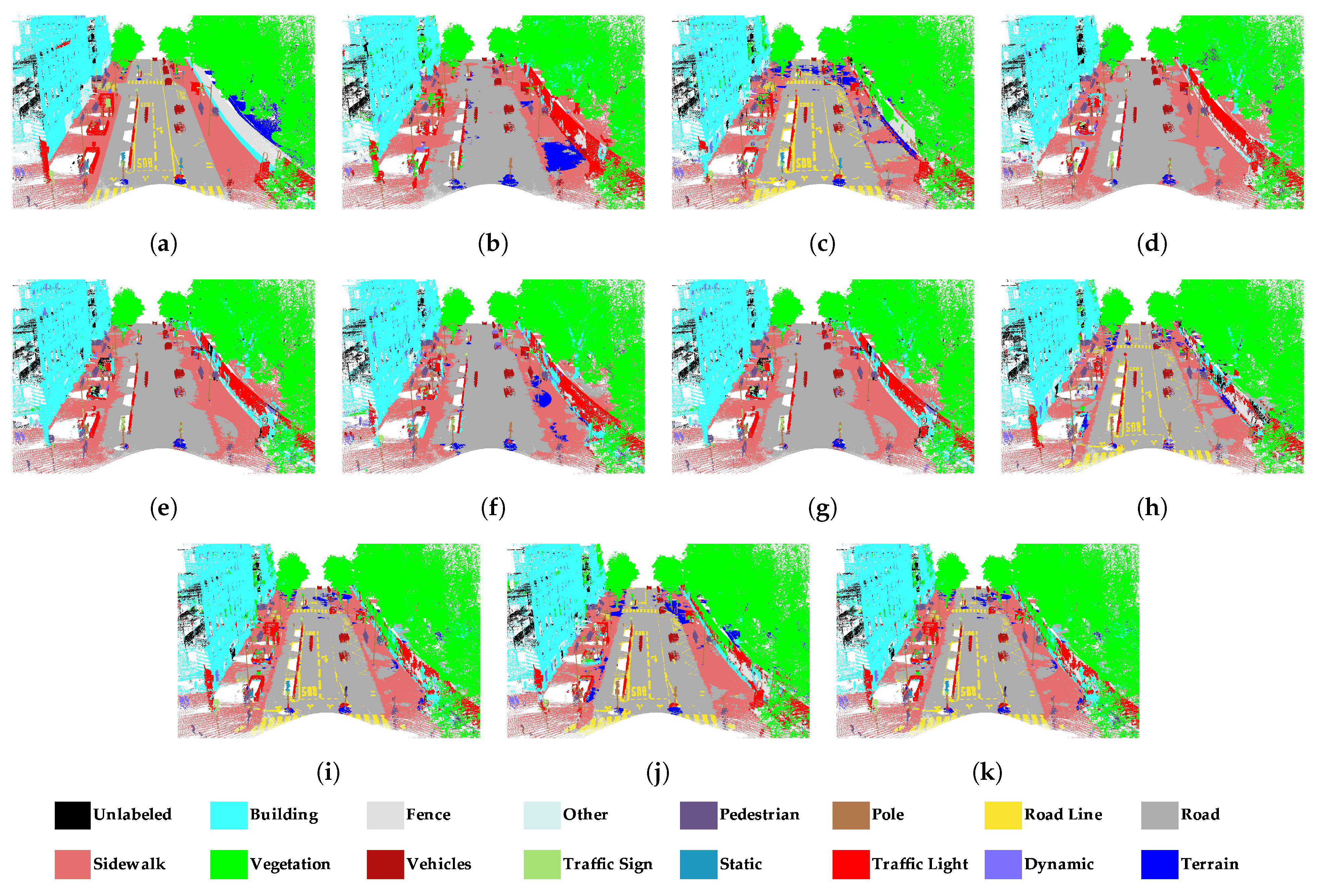
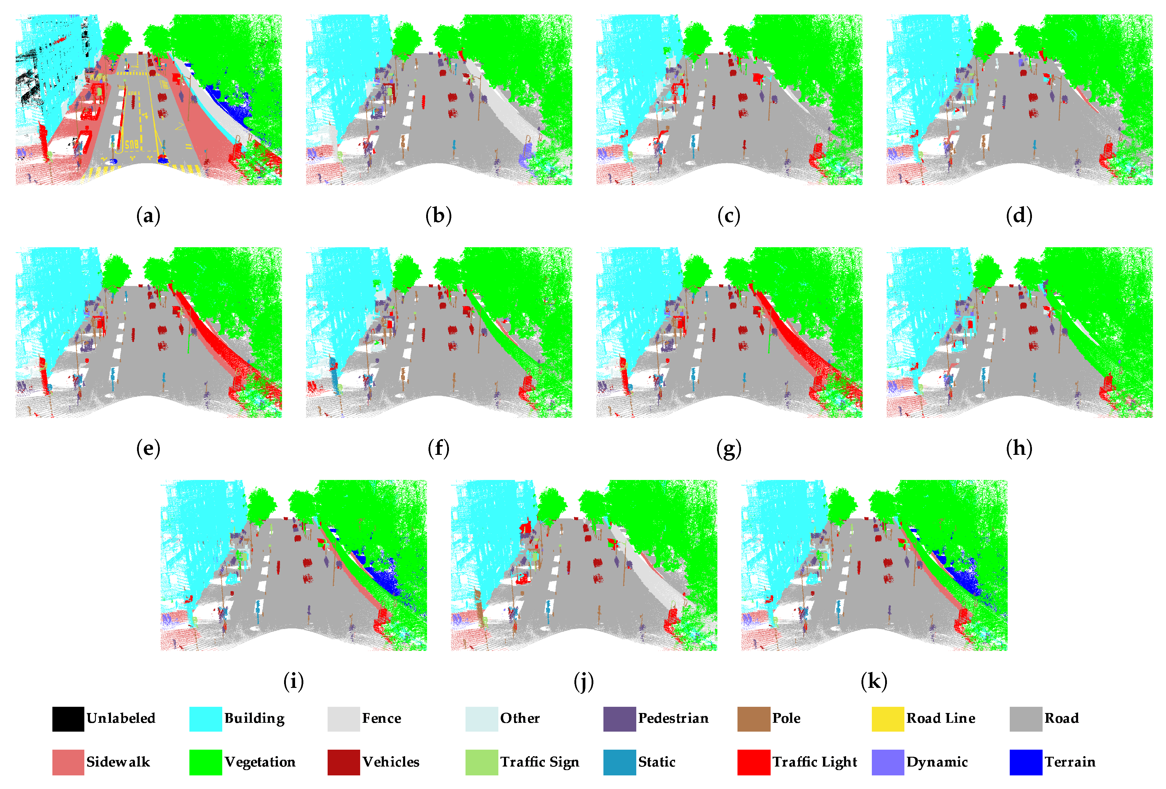
4.4. Results of Semantic Segmentation on Paris

There are many classes with different geometrical structures in the Paris dataset. Successful results were obtained in all subsets in building, road, and vegetation compared to other classes. Since IG and ReliefF select the same features, the results of the subsets created by the two methods are the same. While the road line class has a 0.0 IoU ratio when only geometric features are used, the algorithm can extract the road line class with up to 70% IoU by adding RGB information. IoU increases up to 10% in subsets created by feature selection in the traffic light class. $P_8$ and $P_{1}0$ have 55.2% mIoU. The lowest mIoU with 42.7% was obtained in the $P_1$ subset containing only 3D coordinates (x, y, z). The results of RandLA-Net in the Paris dataset are presented in the

Table 5. Class-based results of RandLA-Net on subsets of Paris. Highest values are marked as bold.

Class	${\mathit{P}}_1$	${\mathit{P}}_2$	${\mathit{P}}_3$	${\mathit{P}}_4$	${\mathit{P}}_5$	${\mathit{P}}_6$	${\mathit{P}}_7$	${\mathit{P}}_8$	${\mathit{P}}_9$	${\mathit{P}}_{10}$
Unlabeled	72.5	67.3	68.4	68.3	72.0	68.3	60.2	72.0	68.9	72.0
Building	85.7	84.9	84.6	85.4	85.5	85.4	83.6	86.1	88.1	86.1
Fence	15.5	22.9	15.9	12.2	16.1	12.2	20.5	22.3	18.9	22.3
Other	22.0	30.2	23.1	20.3	26.0	20.3	27.7	23.5	27.4	23.5
Pedestrian	68.9	58.4	50.7	61.4	64.1	61.4	42.2	60.5	67.9	60.5
Pole	51.3	61.8	48.5	49.6	49.4	49.6	55.0	60.2	56.0	60.2
Road Line	0.0	65.3	0.0	0.0	0.0	0.0	72.3	69.2	70.0	69.2
Road	84.9	86.9	85.1	85.6	83.7	85.6	91.9	91.2	93.2	91.2
Sidewalk	63.7	58.6	63.1	62.1	57.4	62.1	67.5	72.5	60.9	72.5
Vegetation	89.5	84.3	90.2	88.5	91.9	88.5	89.4	86.8	85.6	86.8
Vehicles	75.7	84.2	84.7	84.3	75.2	84.3	77.3	82.0	84.1	82.0
Traffic Sign	0.0	51.8	24.2	21.8	29.0	21.8	34.6	48.1	46.5	48.1
Static	0.0	30.5	2.6	0.0	0.0	0.0	0.0	32.2	0.0	32.2
Traffic Light	33.4	36.0	36.2	46.1	24.6	46.1	38.4	45.7	42.5	45.7
Dynamic	15.1	18.9	14.9	14.2	10.0	14.2	23.4	25.6	28.1	25.6
Terrain	4.2	1.3	5.0	3.8	5.7	3.8	7.5	5.0	6.4	5.0
mIoU	42.7	52.7	43.6	43.9	43.2	43.9	49.5	55.2	52.6	55.2
MA	54.1	68.0	55.0	54.7	53.6	54.7	63.7	67.9	65.5	67.9

. The qualitative assessment of the Paris dataset with RandLA-Net is illustrated in Figure 9.

With the SPG method, high metrics were obtained in the building and vegetation in the Paris dataset. Road class IoU decreased compared to RandLA-Net results. Sidewalk could not be detected in almost any subset. It is usually assigned to the road class. The SPG method could not detect the road line in any of the subsets. Similar to Sidewalk, the road line is mixed with the road class. The terrain class reached 55.8% IoU in $P_8$ and $P_{10}$ subsets, which consist of features selected with IG and RelieF algorithms. The IoU of the fence class decreased when all geometric features were used, but increased when feature selection was applied. The vehicles class reached the highest IoU with 87.0% and 91.6% IoU, respectively, in $P_5$ and $P_9$ subsets containing features selected with Chi2. The highest accuracy was achieved in the $P_8$ and $P_{10}$ subsets, resulting in 59.0% IoU. The lowest IoU (52.3%) was obtained in the $P_3$ subset, where 3D coordinates and all geometrical properties were used. The Chi2 algorithm has lower metrics than IG and ReliefF in the SPG method, as in RandLA-Net. The results of RandLA-Net in Paris dataset are presented in the

Table 6. Class-based results of SPG on subsets of Paris. Highest values are marked as bold.

Class	${\mathit{P}}_1$	${\mathit{P}}_2$	${\mathit{P}}_3$	${\mathit{P}}_4$	${\mathit{P}}_5$	${\mathit{P}}_6$	${\mathit{P}}_7$	${\mathit{P}}_8$	${\mathit{P}}_9$	${\mathit{P}}_{10}$
Unlabeled	1.9	2.0	2.5	2.7	3.4	2.7	2.5	55.8	2.7	55.8
Building	88.3	86.3	87.4	88.3	87.1	88.3	85.9	87.4	85.8	87.4
Fence	31.1	23.8	0.7	10.6	28.3	10.6	6.1	14.7	14.7	14.7
Other	23.4	17.0	6.3	19.1	24.6	19.1	20.0	11.9	10.5	11.9
Pedestrian	33.4	62.7	59.6	58.3	50.2	58.3	48.2	62.7	73.7	62.7
Pole	56.8	54.7	58.1	58.9	47.9	58.9	54.8	50.9	55.4	50.9
Road Line	0.0	0.0	0.0	0.0	0.0	0.0	0.0	0.0	0.0	0.0
Road	74.6	72.9	73.0	74.6	73.7	74.6	75.2	75.2	74.6	75.2
Sidewalk	0.9	2.1	2.5	0.7	0.2	0.7	2.4	1.2	1.2	1.2
Vegetation	94.7	94.3	94.9	93.9	88.6	93.9	80.9	89.2	93.9	89.2
Vehicles	77.3	88.9	84.6	82.5	87.0	82.5	84.5	86.2	91.6	86.2
Traffic Sign	35.8	23.9	38.8	24.5	22.6	24.5	34.6	41.8	35.7	41.8
Static	30.1	22.3	13.4	34.5	10.4	34.5	24.9	24.9	26.3	24.9
Traffic Light	1.2	33.0	6.7	12.1	19.5	12.1	9.0	9.1	16.7	9.1
Dynamic	4.4	17.3	17.0	6.2	5.9	6.2	20.4	4.5	8.7	4.5
Terrain	1.9	2.0	2.5	2.7	3.4	2.7	2.5	55.8	2.7	55.8
mIoU	53.1	57.5	52.3	54.4	52.6	54.4	52.7	59.0	56.7	59.0
MA	46.1	45.8	43.1	46.4	44.3	46.4	45.9	48.1	45.8	48.1

. The qualitative assessment of Paris dataset with RandLA-Net is illustrated in Figure 10.

5. Discussion

The results of the study allow general inferences to be made regarding the usage of suitable 3D geometric features for deep-learning-based point cloud segmentation.

• When Table 1, Table 2, Table 3, Table 4, Table 5 and Table 6 are examined, it is concluded that the use of geometric features improves IoU and mean accuracy. The RandLA-Net algorithm achieved higher performance in $T_3$, $S_2$, and $P_3$ subsets where 3D coordinates and all 3D geometric features are used together, compared to $T_1$, $S_1$, and $P_1$ subsets containing only 3D point coordinates. In Toronto3D, accuracy metrics have increased in subsets where RGB and 3D geometric features are used together, except for the $T_7$ subset, because there are features that do not positively impact accuracy among 3D geometric features. Obtaining the highest mean accuracy metrics with the $T_8$, $T_9$ and $T_{10}$ subsets applied to the feature selection confirms this situation. Furthermore, the addition of RGB information of the points improves accuracy. $T_2$ has higher mIoU than $T_8$, $T_9$ and $T_{10}$ with an added 3D geometric feature. The main reason for this is that the road marking class is detected more accurately in $T_2$. When the mIoU average of the classes is calculated by subtracting the road marking, $T_2$ has 73.4% mIoU, and $T_8$, $T_9$ and $T_{10}$ have 72.4%, 76.0% and 75.0% mIoU, respectively. Geometric features improve accuracy in many classes, especially when Chi2 and ReliefF algorithms are applied. In the SZTAKI-CityMLS dataset, although two features were eliminated with the IG method in the $S_2$ subset, more successful results were obtained by 3.4% in mIoU and 1.6% in MA than $S_1$, which includes all geometric features. Despite the large number of classes, RandLA-Net has successful results in the Paris dataset. In the $P_7$ subset, which includes all of the RGB and 3D geometric features, there is a decrease in accuracy compared to $P_2$. However, the highest mIoU value is obtained in $P_8$ and $P_{10}$ using the features selected with IG and ReliefF. When 3D coordinates and geometric features are used together, there is no significant metric difference between filter-based algorithms. Since RGB information is advantageous for finding classes such as road line, subsets $P_2$, $P_7$, $P_8$, $P_9$, and $P_{10}$ containing RGB information significantly increased in IoU compared to those without RGB.
• RandLA-Net performed well in the road, building, and natural classes in Toronto3D. However, road marking was confused by the road. As seen in Table 1, road marking IoU values are very low, especially in subsets $T_1$, $T_3$, $T_4$, $T_5$, and $T_7$ without RGB. Road markings cover pavement markings including driving lines, arrows, and pedestrian crossings. These markings do not differ from the road class geometrically. Therefore, it is not possible to distinguish road markings using only 3D geometric features. The main difference between road and road markings is in the RGB information. Therefore, road marking has higher IoU in subsets with RGB compared to others. In the $T_2$ subset, the road marking IoU reached approximately 50%. In the fence class, IoU values are generally below 30%. Because fence class has a fewer numbers of points than the others, it was predicted with lower IoU. In SZTAKI-CityMLS dataset, tram/bus, vegetation, column, ground, and facade classes are predicted correctly in all cases. Here, phantom objects are usually the class with the lowest IoU. Classification of phantom objects is a challenge in MLS point clouds. Phantom objects that exist in point clouds representing temporary objects (vehicles, people, or animals) cannot be used for mapping purposes. Phantom objects are confused with other objects because they have irregular geometric structure. It is quite difficult to detect phantom objects using 3D geometric features. When all geometric features are used in the $S_2$ subset, the IoU of the phantom class decreases. However, the IoU value was significantly increased, with seven features selected by the IG method. It seems that the planarity and linearity features negatively affect the accuracy of the phantom class. Significant improvement in the accuracy of the phantom class has been achieved with optimal feature selection. The pedestrian class is often mixed with other classes located nearby. According to Table 5, building, road, and vegetation were successfully extracted in all subsets with RandLA-Net in Paris dataset. Higher IoU is achieved when RGB information is added to the feature vector for the road line class, as in Toronto3D. The classes with the lowest IoU are fence, other, static, dynamic, and terrain. These classes are often confused with other classes of similar characteristics. Dynamic objects can be assigned to other classes because they are geometrically complex and diverse. While the Terrain class is almost never removed in other subsets, the IoU value reaches 55.8% IoU with the $P_8$ and $P_{10}$ subsets. It is often confused with vegetation and road. $sphericity$ and $planarity$ selected with Chi2 are not enough to distinguish terrain.
• Feature selection improves evaluation metrics in all datasets in the semantic segmentation performed with SPG. Adding RGB or geometric features in the Toronto3D dataset increases the accuracy of semantic segmentation. Chi2 is superior to other methods in semantic segmentation of Toronto3D with SPG. The mIoU of $T_5$ is 1.2% higher than $T_3$, which includes all geometric features, and the mIoU of $T_9$ is 2.8% higher than $T_7$, which includes RGB and all geometric features. Features selected with ReliefF reduce the semantic segmentation accuracy of SPG in Toronto3D. In SZTAKI-CityMLS, the highest accuracy was obtained in the $S_3$ subset created with the features selected with IG. In the Paris dataset, as in RandLA-Net, the highest mIoU was obtained in $P_8$ and $P_{10}$ created with IG and ReliefF. Generally, the subset results are similar to RandLA-Net. Thus, it was concluded that the features determined via filter-based methods have similar effects in different algorithms.
• Road markings are assigned as road. Since road and road marking (line) have the same geometric structure, they cannot be distinguished by SPG, which mostly uses geometric relationships. The most significant differences between the subsets in the Toronto3D dataset occur in the fence class. Adding RGB information in particular increases the IoU of the car class. Although SPG has a better result in determining the phantom class in SZTAKI-CityMLS, some points belonging to the tram/bus class are assigned to the phantom class. IoU increased in most classes with IG, while it decreased with ReliefF.
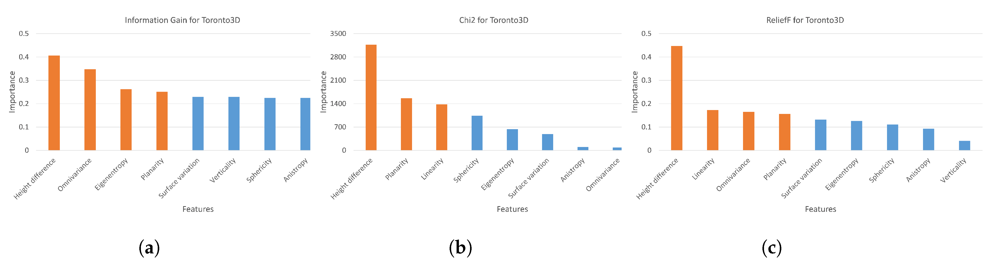
• IG and Chi2 algorithms performed more successful feature selection in the Toronto3D dataset. Semantic segmentation with features determined by ReliefF has lower accuracy. According to the results presented in Figure 2, ReliefF calculated the effect of features other than height difference as both very low and close to each other. In addition, although similar features have high importance, it was concluded that the combination of features is important for semantic segmentation. Although there is only one feature difference between $T_4$ and $T_6$, an increase of approximately 3% mIoU and 1.6% MA is achieved with $T_4$. Even though only the omnivariance feature was added in $T_6$, mIoU decreased by 1.2% and MA by 4.2% compared to $T_5$. When RGB is added to the selected features, the highest metrics $T_9$ created with Chi2 are obtained. In the semantic segmentation of the SZTAKI-CityMLS dataset, the positive effect of 3D geometric features on accuracy is seen more clearly. All other subsets containing 3D geometric features are superior to the dataset $S_1$, which contains only the 3D coordinates of the points. Although there is no significant difference between filter-based algorithms when only selected geometric features are used, when RGB information is added, approximately 2.5% improvement in mIoU is achieved in subsets created with features selected by IG and ReliefF algorithms compared to Chi2 in Paris dataset.
• However, instead of using all of the geometric features, the results are more successful when the most suitable ones are selected with feature selection. Although all geometric features were used in the subsets $T_3$, $T_7$, $S_1$, $P_3$, and $P_7$, the highest metrics could not be obtained. Some of the features can negatively affect semantic segmentation. For this reason, applying feature selection methods enabled the development of semantic segmentation results by eliminating unnecessary features. This is confirmed by the results of the study.

6. Conclusions

In this study, the effect of using 3D geometric features for deep-learning-based semantic segmentation of mobile point clouds was examined, and appropriate feature selection was carried out. The performances of three filter-based methods for feature selection (IG, Chi2 and ReliefF) were compared on two different datasets. RandLA-Net and SPG were used as a deep learning network. For the semantic segmentation of Mobile LiDAR point clouds, we obtained the following conclusions by comparing the 3D coordinate information, geometric features, spectral features, and feature subsets created using filter-based methods.

• Using all geometric features does not guarantee better results. Feature selection methods improve semantic segmentation accuracy by identifying suitable features. This improvement becomes even more evident, especially if there are geometrical differences between classes. The usage of effective geometric features provides an advantage in semantic segmentation.
• Successful results were obtained by selecting features with the IG method in all datasets. Thanks to the feature selection with the Chi2 method, the highest mean accuracy is obtained in Toronto3D, while the IG method is more successful than Chi2 in the SZTAKI-CityMLS and Paris datasets. The feature selection problem may differ depending on the dataset. The fact that the datasets are different and the datasets have different features related to each other causes the appropriate feature selection method to change. Similar feature selection algorithms can be used for datasets with similar features.
• Evaluation metrics increase if spectral information is used together with 3D geometric features. Spectral features are useful for separating features such as road lines.
• Mobile point clouds are often captured in a dynamic environment. Future studies will focus on eliminating the noise caused by dynamic objects (moving car, moving pedestrian, other living beings, etc.) in the mobile LiDAR point clouds.

References

1. Bello, S.A.; Yu, S.; Wang, C.; Adam, J.M.; Li, J. Review: Deep learning on 3D point clouds. Remote Sens. 2020, 12, 1729. [Google Scholar] [CrossRef]
2. Griffiths, D.; Boehm, J. A Review on deep learning techniques for 3D sensed data classification. Remote Sens. 2019, 11, 1499. [Google Scholar] [CrossRef] [Green Version]
3. Guo, Y.; Wang, H.; Hu, Q.; Liu, H.; Liu, L.; Bennamoun, M. Deep Learning for 3D Point Clouds: A Survey. IEEE Trans. Pattern Anal. Mach. Intell. 2021, 43, 4338–4364. [Google Scholar] [CrossRef]
4. Duran, Z.; Aydar, U. Digital modeling of world’s first known length reference unit: The Nippur cubit rod. J. Cult. Herit. 2012, 13, 352–356. [Google Scholar] [CrossRef]
5. Hoang, L.; Lee, S.H.; Lee, E.J.; Kwon, K.R. GSV-NET: A Multi-Modal Deep Learning Network for 3D Point Cloud Classification. Appl. Sci. 2022, 12, 483. [Google Scholar] [CrossRef]
6. He, Y.; Chen, W.; Li, C.; Luo, X.; Huang, L. Fast and accurate lane detection via graph structure and disentangled representation learning. Sensors 2021, 21, 4657. [Google Scholar] [CrossRef]
7. Wu, B.; Zhou, X.; Zhao, S.; Yue, X.; Keutzer, K. SqueezeSegV2: Improved model structure and unsupervised domain adaptation for road-object segmentation from a LiDAR point cloud. In Proceedings of the IEEE International Conference on Robotics and Automation (ICRA), Montreal, QC, Canada, 20–24 May 2019; pp. 4376–4382. [Google Scholar]
8. Akyol, O.; Duran, Z. Low-Cost Laser Scanning System Design. J. Russ. Laser Res. 2014, 35, 244–251. [Google Scholar] [CrossRef]
9. Rim, B.; Lee, A.; Hong, M. Semantic segmentation of large-scale outdoor point clouds by encoder–decoder shared mlps with multiple losses. Remote Sens. 2021, 13, 3121. [Google Scholar] [CrossRef]
10. Weinmann, M.; Jutzi, B.; Hinz, S.; Mallet, C. Semantic point cloud interpretation based on optimal neighborhoods, relevant features and efficient classifiers. ISPRS J. Photogramm. Remote Sens. 2015, 105, 286–304. [Google Scholar] [CrossRef]
11. Atik, M.E.; Duran, Z.; Seker, D.Z. Machine learning-based supervised classification of point clouds using multiscale geometric features. ISPRS Int. J. Geo-Inf. 2021, 10, 187. [Google Scholar] [CrossRef]
12. Atik, M.E.; Duran, Z. Classification of Aerial Photogrammetric Point Cloud Using Recurrent Neural Networks. Fresenius Environ. Bull. 2021, 30, 4270–4275. [Google Scholar]
13. Ronneberger, O.; Fischer, P.; Brox, T. U-Net: Convolutional Networks for Biomedical Image Segmentation. In Proceedings of the International Conference on Medical Image Computing and Computer-Assisted Intervention, Munich, Germany, 5–9 October 2015; Springer: Cham, Switzerland; pp. 234–241. [Google Scholar]
14. Atik, S.O.; Ipbuker, C. Building Extraction in VHR Remote Sensing Imagery Through Deep Learning. Fresenius Environ. Bull. 2022, 31, 8468–8473. [Google Scholar]
15. Badrinarayanan, V.; Kendall, A.; Cipolla, R. SegNet: A Deep Convolutional Encoder-Decoder Architecture for Image Segmentation. IEEE Trans. Pattern Anal. Mach. Intell. 2017, 39, 2481–2495. [Google Scholar] [CrossRef]
16. Atik, S.O.; Ipbuker, C. Integrating convolutional neural network and multiresolution segmentation for land cover and land use mapping using satellite imagery. Appl. Sci. 2021, 11, 5551. [Google Scholar] [CrossRef]
17. Atik, S.O.; Atik, M.E.; Ipbuker, C. Comparative research on different backbone architectures of DeepLabV3+ for building segmentation. J. Appl. Remote Sens. 2022, 16, 024510. [Google Scholar] [CrossRef]
18. Hu, Q.; Yang, B.; Xie, L.; Rosa, S.; Guo, Y.; Wang, Z.; Trigoni, N.; Markham, A. Randla-Net: Efficient semantic segmentation of large-scale point clouds. In Proceedings of the IEEE/CVF Conference on Computer Vision and Pattern Recognition, Seattle, DC, USA, 16–18 June 2020; pp. 11108–11117. [Google Scholar]
19. Landrieu, L.; Simonovsky, M. Large-Scale Point Cloud Semantic Segmentation with Superpoint Graphs. arXiv 2017, arXiv:1711.09869. [Google Scholar]
20. Liu, H.; Setiono, R. Chi2: Feature selection and discretization of numeric attributes. In Proceedings of the Seventh IEEE International Conference on Tools with Artificial Intelligence, Herndon, VA, USA, 29–31 May 1995; pp. 388–391. [Google Scholar]
21. Robnik-Šikonja, M.; Kononenko, I. Theoretical and Empirical Analysis of ReliefF and RReliefF. Mach. Learn. 2003, 53, 23–69. [Google Scholar] [CrossRef] [Green Version]
22. Tan, W.; Qin, N.; Ma, L.; Li, Y.; Du, J.; Cai, G.; Yang, K.; Li, J. Toronto-3D: A large-scale mobile LiDAR dataset for semantic segmentation of urban roadways. arXiv 2020, arXiv:2003.08284. [Google Scholar]
23. Nagy, B.; Benedek, C. 3D CNN-based semantic labeling approach for mobile laser scanning data. IEEE Sens. J. 2019, 19, 7269. [Google Scholar] [CrossRef] [Green Version]
24. Deschaud, J.E.; Duque, D.; Richa, J.P.; Velasco-Forero, S.; Marcotegui, B.; Goulette, F. Paris-CARLA-3D: A Real and Synthetic Outdoor Point Cloud Dataset for Challenging Tasks in 3D Mapping. Remote Sens. 2021, 13, 4713. [Google Scholar] [CrossRef]
25. Lawin, F.J.; Danelljan, M.; Tosteberg, P.; Bhat, G.; Khan, F.S.; Felsberg, M. Deep projective 3D semantic segmentation. In Proceedings of the 2017 International Conference on Computer Analysis of Images and Patterns, Ystad, Sweden, 22–24 August 2017; pp. 95–107. [Google Scholar]
26. Meng, H.Y.; Gao, L.; Lai, Y.K.; Manocha, D. VV-net: Voxel VAE net with group convolutions for point cloud segmentation. In Proceedings of the IEEE/CVF International Conference on Computer Vision, Seoul, Korea, 27–28 October 2019; pp. 8500–8508. [Google Scholar]
27. Qi, C.R.; Su, H.; Mo, K.; Guibas, L.J. PointNet: Deep learning on point sets for 3D classification and segmentation. In Proceedings of the 30th IEEE Conference on Computer Vision and Pattern Recognition, Las Vegas, NV, USA, 27–30 June 2016; pp. 77–85. [Google Scholar]
28. Qi, C.R.; Yi, L.; Su, H.; Guibas, L.J. PointNet++: Deep hierarchical feature learning on point sets in a metric space. In Proceedings of the Advances in Neural Information Processing Systems, Long Beach, CA, USA, 4–9 December 2017; pp. 5105–5114. [Google Scholar]
29. Jiang, M.; Wu, Y.; Zhao, T.; Zhao, Z.; Lu, C. PointSIFT: A SIFT-like Network Module for 3D Point Cloud Semantic Segmentation. arXiv 2018, arXiv:1807.00652. [Google Scholar]
30. Lowe, G. SIFT—The Scale Invariant Feature Transform. Int. J. Comput. Vis. 2004, 2, 91–110. [Google Scholar] [CrossRef]
31. Engelmann, F.; Kontogianni, T.; Schult, J.; Leibe, B. Know what your neighbors do: 3D semantic segmentation of point clouds. In Proceedings of the European Conference on Computer Vision (ECCV) Workshops, Munich, Germany, 8–14 September 2018. [Google Scholar]
32. Zhao, H.; Jiang, L.; Fu, C.W.; Jia, J. Pointweb: Enhancing local neighborhood features for point cloud processing. In Proceedings of the IEEE Conference on Computer Vision and Pattern Recognition (CVPR), Long Beach, CA, USA, 16–20 June 2019; pp. 5565–5573. [Google Scholar]
33. Zhang, Z.; Hua, B.S.; Yeung, S.K. ShellNet: Efficient point cloud convolutional neural networks using concentric shells statistics. In Proceedings of the IEEE International Conference on Computer Vision, Thessaloniki, Greece, 23–25 September 2019; Institute of Electrical and Electronics Engineers Inc.: New York, NY, USA, 2019; pp. 1607–1616. [Google Scholar]
34. Thomas, H.; Qi, C.R.; Deschaud, J.E.; Marcotegui, B.; Goulette, F.; Guibas, L. KPConv: Flexible and deformable convolution for point clouds. arXiv 2019, arXiv:1904.08889. [Google Scholar]
35. Li, Y.; Bu, R.; Sun, M.; Wu, W.; Di, X.; Chen, B. PointCNN: Convolution on X-transformed points. In Advances in Neural Information Processing Systems 31; Bengio, S., Wallach, H., Larochelle, H., Grauman, K., Cesa-Bianchi, N., Garnett, R., Eds.; Curran Associates, Inc.: Red Hook, NY, USA, 2018; pp. 820–830. [Google Scholar]
36. Xu, Y.; Fan, T.; Xu, M.; Zeng, L.; Qiao, Y. SpiderCNN: Deep learning on point sets with parameterized convolutional filters. In Proceedings of the European Conference on Computer Vision, Munich, Germany, 8–14 September 2018. [Google Scholar]
37. Boulch, A. ConvPoint: Continuous convolutions for point cloud processing. Comput. Graph. 2020, 88, 24–34. [Google Scholar] [CrossRef] [Green Version]
38. Zhou, H.; Feng, Y.; Fang, M.; Wei, M.; Qin, J.; Lu, T. Adaptive Graph Convolution for Point Cloud Analysis. In Proceedings of the IEEE/CVF International Conference on Computer Vision, Virtual, 19–25 June 2021; pp. 4965–4974. [Google Scholar]
39. Wang, Y.; Sun, Y.; Liu, Z.; Sarma, S.E.; Bronstein, M.M.; Solomon, J.M. Dynamic graph Cnn for learning on point clouds. ACM Trans. Graph. 2019, 38, 1–12. [Google Scholar] [CrossRef] [Green Version]
40. Lin, Z.H.; Huang, S.Y.; Wang, Y.C.F. Convolution in the cloud: Learning deformable kernels in 3D graph convolution networks for point cloud analysis. In Proceedings of the IEEE/CVF Conference on Computer Vision and Pattern Recognition, Seattle, WA, USA, 13–19 June 2020; pp. 1800–1809. [Google Scholar]
41. Liu, J.; Ni, B.; Li, C.; Yang, J.; Tian, Q. Dynamic points agglomeration for hierarchical point sets learning. Proc. IEEE Int. Conf. Comput. Vis. 2019, 2019, 7545–7554. [Google Scholar]
42. Maturana, D.; Scherer, S. VoxNet: A 3D Convolutional Neural Network for real-time object recognition. In Proceedings of the 2015 IEEE/RSJ International Conference on Intelligent Robots and Systems (IROS), Hamburg, Germany, 28 September–3 October 2015; pp. 922–928. [Google Scholar]
43. Liao, L.; Tang, S.; Liao, J.; Li, X.; Wang, W.; Li, Y.; Guo, R. A Supervoxel-Based Random Forest Method for Robust and Effective Airborne LiDAR Point Cloud Classification. Remote Sens. 2022, 14, 1516. [Google Scholar] [CrossRef]
44. Choy, C.; Gwak, J.; Savarese, S. 4D Spatio-Temporal ConvNets: Minkowski Convolutional Neural Networks. In Proceedings of the IEEE Conference on Computer Vision and Pattern Recognition, Long Beach, CA, USA, 16–20 June 2019; pp. 3075–3084. [Google Scholar]
45. Iandola, F.N.; Han, S.; Moskewicz, M.W.; Ashraf, K.; Dally, W.J.; Keutzer, K. SqueezeNet: AlexNet-level accuracy with 50x fewer parameters and <0.5 MB model size. arXiv 2016, arXiv:1602.07360. [Google Scholar]
46. Wu, B.; Wan, A.; Yue, X.; Keutzer, K. SqueezeSeg: Convolutional Neural Nets with Recurrent CRF for Real-Time Road-Object Segmentation from 3D LiDAR Point Cloud. In Proceedings of the 2018 IEEE International Conference on Robotics and Automation (ICRA), Brisbane, Australia, 21–25 May 2018; pp. 1887–1893. [Google Scholar]
47. Milioto, A.; Vizzo, I.; Behley, J.; Stachniss, C. RangeNet ++: Fast and Accurate LiDAR Semantic Segmentation. In Proceedings of the IEEE International Conference on Intelligent Robots and Systems, Macau, China, 4–8 November 2019; IEEE: New York, NY, USA, 2019; pp. 4213–4220. [Google Scholar]
48. Cortinhal, T.; Tzelepis, G.; Aksoy, E.E. SalsaNext: Fast, Uncertainty-Aware Semantic Segmentation of LiDAR Point Clouds. In Advances in Visual Computing ISVC 2020 Lecture Notes in Computer Science; Bebis, G., Ed.; Springer: Cham, Switzerland, 2020; Volume 12510, pp. 207–222. [Google Scholar]
49. Aksoy, E.E.; Baci, S.; Cavdar, S. SalsaNet: Fast Road and Vehicle Segmentation in LiDAR Point Clouds for Autonomous Driving. In Proceedings of the 2020 IEEE Intelligent Vehicles Symposium (IV), Paris, France, 9–12 June 2019; pp. 926–932. [Google Scholar]
50. Biasutti, P.; Lepetit, V.; Aujol, J.F.; Bredif, M.; Bugeau, A. LU-net: An efficient network for 3D LiDAR point cloud semantic segmentation based on end-to-end-learned 3D features and U-net. In Proceedings of the IEEE/CVF International Conference on Computer Vision Workshops, Seoul, Korea, 27–28 October 2019. [Google Scholar]
51. Atik, M.E.; Duran, Z. An Efficient Ensemble Deep Learning Approach for Semantic Point Cloud Segmentation Based on 3D Geometric Features and Range Images. Sensors 2022, 22, 6210. [Google Scholar] [CrossRef] [PubMed]
52. Jaritz, M.; Gu, J.; Su, H. Multi-view PointNet for 3D Scene Understanding. In Proceedings of the IEEE/CVF International Conference on Computer Vision (ICCVW), Seoul, Korea, 1 October 2019; pp. 3995–4003. [Google Scholar]
53. Meng, Q.; Wang, W.; Zhou, T.; Shen, J.; Jia, Y.; Van Gool, L. Towards a Weakly Supervised Framework for 3D Point Cloud Object Detection and Annotation. IEEE Trans. Pattern Anal. Mach. Intell. 2022, 44, 4454–4468. [Google Scholar] [CrossRef]
54. Wu, B.; Chen, C.; Kechadi, T.M.; Sun, L. A comparative evaluation of filter-based feature selection methods for hyper-spectral band selection. Int. J. Remote Sens. 2013, 34, 7974–7990. [Google Scholar] [CrossRef]
55. Lei, S. A feature selection method based on information gain and genetic algorithm. In Proceedings of the 2012 International Conference on Computer Science and Electronics Engineering, Hangzhou, China, 23–25 March 2012; Volume 2, pp. 355–358. [Google Scholar]
56. Colkesen, I.; Kavzoglu, T. Selection of Optimal Object Features in Object-Based Image Analysis Using Filter-Based Algorithms. J. Indian Soc. Remote Sens. 2018, 46, 1233–1242. [Google Scholar] [CrossRef]
57. Kononenko, I. Estimating attributes: Analysis and extensions of RELIEF. In Proceedings of the European Conference on Machine Learning; Springer: Catania, Italy, 1994; pp. 171–182. [Google Scholar]
58. Duran, Z.; Ozcan, K.; Atik, M.E. Classification of photogrammetric and airborne lidar point clouds using machine learning algorithms. Drones 2021, 5, 104. [Google Scholar] [CrossRef]
59. Pedregosa, F.; Gramfort, N.A.; Michel, V.; Thirion, B.; Grisel, O.; Blondel, M.; Prettenhofer, P.; Weiss, R.; Dubourg, V.; Vanderplas, J.; et al. Scikit-learn: Machine Learning in Python. J. Mach. Learn. Res. 2011, 12, 2825–2830. [Google Scholar]
60. Holmes, G.; Donkin, A.; Witten, I.H. WEKA: A machine learning workbench. In Proceedings of the ANZIIS ’94—Australian New Zealnd Intelligent Information Systems Conference, Brisbane, Australia, 29 November–2 December 1994. [Google Scholar]
61. Zhou, Q.Y.; Park, J.; Koltun, V. Open3D: A Modern Library for 3D Data Processing. arXiv 2018, arXiv:1801.09847. [Google Scholar]
Figure 1. Workflow of the study.
Electronics 11 03310 g001
Figure 2. Importance of each feature by filter-based feature selection algorithms for Toronto3D. Selected features are marked as orange. (a) Feature importance calculated with IG (b) Feature importance calculated with Chi2. (c) Feature importance calculated with ReliefF.
Electronics 11 03310 g002
Figure 3. Importance of each feature calculated using filter-based feature selection algorithms for SZTAKI-CityMLS. Selected features are marked as orange. (a) Feature importance calculated with IG (b) Feature importance calculated with Chi2. (c) Feature importance calculated with ReliefF.
Electronics 11 03310 g003
Figure 4. Importance of each feature by filter-based feature selection algorithms for Paris. Selected features are marked as orange. (a) Feature importance calculated with IG (b) Feature importance calculated with Chi2. (c) Feature importance calculated with ReliefF.
Electronics 11 03310 g004
Figure 5. Qualitative results of the methods for Toronto3D with RandLA-Net. (a) Ground Truth; (b) T 1 ; (c) T 2 ; (d) T 3 ; (e) T 4 ; (f) T 5 ; (g) T 6 ; (h) T 7 ; (i) T 8 ; (j) T 9 ; (k) T 10 .
Electronics 11 03310 g005
Figure 6. Qualitative results of the methods for Toronto3D with SPG. (a) Ground Truth; (b) T 1 ; (c) T 2 ; (d) T 3 ; (e) T 4 ; (f) T 5 ; (g) T 6 ; (h) T 7 ; (i) T 8 ; (j) T 9 ; (k) T 10 .
Electronics 11 03310 g006
Figure 7. Qualitative results of the methods for SZTAKI-CityMLS with RandLA-Net. (a) Ground Truth; (b) S 1 ; (c) S 2 ; (d) S 3 ; (e) S 4 ; (f) S 5 .
Electronics 11 03310 g007
Figure 8. Qualitative results of the methods for SZTAKI-CityMLS with SPG. (a) Ground Truth; (b) S 1 ; (c) S 2 ; (d) S 3 ; (e) S 4 ; (f) S 5 .
Electronics 11 03310 g008
Figure 9. Qualitative results of the methods for Paris dataset with RandLA-Net. (a) Ground Truth; (b) P 1 ; (c) P 2 ; (d) P 3 ; (e) P 4 ; (f) P 5 ; (g) P 6 ; (h) P 7 ; (i) P 8 ; (j) P 9 ; (k) P 10 .
Electronics 11 03310 g009
Figure 10. Qualitative results of the methods for Paris dataset with SPG. (a) Ground Truth; (b) P 1 ; (c) P 2 ; (d) P 3 ; (e) P 4 ; (f) P 5 ; (g) P 6 ; (h) P 7 ; (i) P 8 ; (j) P 9 ; (k) P 10 .
Electronics 11 03310 g010